Redundancy or Mismeasurement? A Reappraisal of Money Joshua R. Hendrickson∗
Forthcoming, Macroeconomic Dynamics Abstract The emerging consensus in monetary policy and business cycle analysis is that money aggregates are not useful as an intermediate target for monetary policy or as an information variable. The uselessness of money as an intermediate target is driven, at least in part, by empirical research that suggests that money demand is unstable. In addition, the informational quality of money has been called into question by empirical research that fails to identify a relationship between money growth and inflation, nominal income growth, and the output gap. Nevertheless, this research is potentially flawed by the use of simple sum money aggregates, which are not consistent with economic, aggregation, or index number theory. This paper therefore re-examines previous empirical evidence on money demand and the role of money as an information variable using Divisia monetary aggregates. These aggregates have the advantage of being derived from microtheoretic foundations as well as being consistent with aggregation and index number theory. The results of the re-evaluation suggest that previous empirical work might be driven by mismeasurement.
JEL codes: E31, E32, E41, E51 Keywords: monetary aggregates; money; business cycles; money demand; cointegrated VAR
∗ Joshua R. Hendrickson: University of Mississippi, Department of Economics, 229 North Hall, University, MS, 38677
[email protected]. This paper was adapted from a chapter of the author’s Ph.D. dissertation. The author would like to thank Robert Rossana, Ana Mar´ıa Herrera, and Yong-Gook Jung, as well as seminar participants at Bentley University and the University of Mississippi for comments on an earlier draft. The author would also like to thank the associate editor and two anonymous referees for helpful comments. The usual caveat applies.
1
1
Introduction
The extant consensus in the literature on monetary policy and business cycles is that money aggregates can be altogether ignored without the loss of significant information. The justification for this consensus is based on four factors. First, the Federal Reserve and other central banks around the world use an interest rate as their intermediate target for monetary policy. While this does not necessarily rule out a role for monetary aggregates in monetary policy analysis, it is not clear a priori whether these aggregates provide additional information not communicated by movements in the interest rate. Second, there is a widespread belief that the demand for money is unstable (Friedman and Kuttner (1992); Estrella and Mishkin (1997)) and as a result monetary aggregates do not have a predictable influence on other economic variables.1 Third, empirical estimation of backward-looking IS equations do not find a statistically significant relationship between real money balances and the output gap (Rudebusch and Svensson, 2002). Finally, the dynamic New Keynesian model, which is the workhorse of modern monetary policy research, abstracts from money completely based on the claim that money is redundant in the model.2 In fact, McCallum (2001) notes that the quantitative implications of this omission are quite small. The purpose of this paper is to examine whether these results are robust to the method of aggregation used to create monetary aggregates. The paper proceeds as follows. Section 2 outlines the traditional role for monetary aggregates, discusses existing empirical evidence, and posits the hypothesis that previous empirical results are driven by simple sum aggregation. Sections 3 reexamines previous empirical models by contrasting the results obtained with simple sum aggregates to those estimated with theoretically superior monetary aggregates. Section 4 concludes.
2
Monetary Aggregates and Monetary Policy
2.1
The Role of Monetary Aggregates
Money typically has one of three roles in empirical analysis: a study of the demand for money, a study of the role of money in forecasting inflation and/or nominal income, and more recently 1
This paper adopts the definition of stability used by Friedman and Kuttner (1992). Specifically, money demand is stable if there exists an identified money demand equation in a cointegrated VAR model. This is an admittedly strict definition and one that is addressed in Section 3.1.2 below. 2 For a textbook treatment, see Woodford (2003) or Gali (2008).
2
studies explaining movements in the output gap. These studies are motivated as follows. First, analysis of money demand is important because it is a widely accepted axiom that the existence of a stable money demand function is necessary for money to have a predictable influence on other economic variables. Second, any type of quantity-theoretic analysis implies that money should predict movements in the price level and nominal income. Finally, the short-run non-neutrality of money has recently been analyzed in the context of an IS equation to assess whether real money balances can explain movements in the output gap. As noted above, the emerging consensus in the literature is that money is not useful in the conduct or evaluation of monetary policy. This section outlines three empirical methods that have been used to examine the characteristics of money described above.
2.1.1
Money Demand Stability
A traditional money demand function take the form:
mt − pt = β0 + β1 yt + β2 Rt + et
(1)
where mt − pt denotes real money balances, yt is a scale variable of real economic activity, Rt is a price variable, et is a disturbance, and βi are parameters. Given that each of the variables in the money demand function are non-stationary I(1), they have no tendency to return to a long-run level. Nevertheless, it remains possible that there is a stable long-run money demand function. For example, this will be the case if et follows a stationary process. This will be the case if the I(1) variables are cointegrated, or share a common stochastic trend. Friedman and Kuttner (1992) examine the stability of money demand by testing for cointegration for three separate quarterly samples: 1960:2 - 1979:3, 1960:2 - 1990:4, and 1970:3 - 1990:4. The use of three separate samples is motivated by the hypothesis that financial innovation and changes in monetary policy might disrupt the relationship between real money balances and other economic variables therefore impeding the usefulness of monetary aggregates in the conduct and evaluation of monetary policy. In addition, they consider three measures of money: the monetary base, M1, and M2. For the first sample period, the authors find evidence of cointegration for each of the monetary
3
aggregates. In the second sample period, evidence of cointegration is found only for M2. Finally, in the last sample period, there is no evidence of cointegration for any measure of money. As a result, Friedman and Kuttner (1992: 490) conclude that, “whatever the situation may have been before the 1980’s, it is no longer possible to discern from the data a stable long-run relationship between income and the monetary base, M1, or credit, either with or without allowance for the effect of interest rates, and the evidence of such stability in the case of M2 strictly depends on the inclusion of data from the 1960’s.” Broadly, this can be interpreted as a breakdown in the stability of money demand.
2.1.2
Money, Inflation, and Nominal Income
The second traditional role for money in empirical analysis is an examination of the ability of monetary aggregates to predict nominal income and the price level. Estrella and Mishkin (1997) estimated a three variable vector autoregressive (VAR) model consisting of nominal income growth, inflation, and money growth for a sample ranging from 1960 - 1995. They also estimate the model for the subsample beginning in October 1979, which coincides with the emergency meeting of the Federal Reserve in which it adopted an intermediate target for M1. Money growth is measured by the monetary base and M2. Using this model, they conduct Granger causality tests to determine whether money growth can predict nominal income growth and inflation. The results of the Granger causality tests suggest that, for the entire sample, the monetary base is useful in predicting nominal income growth and inflation whereas M2 is useful in predicting nominal income growth. For the subsample, however, neither the growth of the monetary base nor M2 is useful in predicting nominal income growth and inflation. These results imply that monetary aggregates are not useful as information variables after October 1979.
2.1.3
Money and the Output Gap
More recently, there has been a focus on the impact of money on aggregate demand. Formally, this role can be examined within the context of an IS equation. Rudebusch and Svensson (2002) estimate a backward-looking IS equation of the form:
yt = β1 yt−1 + β2 yt−2 + β3 (it−1 − πt−1 ) + εt 4
(2)
where y is the output gap defined as the percentage deviation of real output from the Congressional Budget Office’s measure of potential, i is the federal funds rate, and π is the average rate of inflation rate as measured by the GDP deflator. The parameter estimates are obtained using a sample of quarterly data from 1961 - 1996. They find that the output gap has a strong autoregressive component and is negatively related to the lagged real interest. All three parameters are statistically significant and they report that these estimates are stable over time.3 Notably missing from this analysis is money as the authors (ibid: 423) acknowledge that, “lags of nominal money (in levels or growth rates) were insignificant when added” to the IS equation above.4 These findings are important because they have been used to justify the exclusion of money from the New Keynesian model, which has become the workhorse of monetary policy analysis.
2.2
Does Measurement Matter?
The results above present a bleak outlook for the use of monetary aggregates in the conduct and evaluation of monetary policy. Nevertheless, this evidence relies on the use of simple sum monetary aggregates in which different monetary components are added together with equal weights. This procedure has long been considered inadequate for measuring money.5 For example, in assessing different measures of money included in their Monetary Statistics of the United States, Friedman and Schwartz (1970: 151) noted that it would be more appropriate for the components of money aggregates to be assigned a weight based on their degree of “moneyness.” The reason that the weights of each asset are important is because the simple sum money aggregates imply that each asset is a perfect substitute for all other assets in the index. This is problematic because it is contrary to empirical evidence and as a result simple sum aggregates fail to capture pure substitution effects across assets.6 The failure of simple sum aggregates to capture these substitution effects is important as it necessarily implies that there has been some change in the subutility function pertaining to monetary services and, potentially, the observed instability of money demand discussed above. 3
The specific results are listed below in direct comparison to the empirical analysis in this paper. Their focus on nominal money is a bit curious as traditional Monetarist analysis emphasizes changes in real money balances. 5 The earliest critic of simple arithmetic index numbers is Fisher (1922). 6 Cf. Barnett, Fisher, and Serletis (1992), Serletis (2001). 4
5
An alternative to the simple sum indexes are the Divisia monetary aggregates derived by Barnett (1980) in which the components of the monetary aggregate are weighted by their expediture share. In contrast to the simple sum aggregates, the Divisia aggregates are derived from microtheoretic foundations and are also consistent with index number and aggregation theory. The theoretical superiority of the Divisia aggregates raises questions about empirical results using simple sum aggregates. Given that the simple sum aggregates are not consistent with economic, index number, or aggregation theory, it is possible that empirical estimates using these aggregates are potentially flawed due to improper aggregation. There exists empirical evidence to support this hypothesis. For example, Belongia (1996) re-examines five puzzling results from the monetary literature by utilizing Divisia aggregates rather than the simple sum counterparts. He finds that four of the five puzzling results exist only when the simple sum aggregates are used. The results for the fifth puzzle are mixed. In addition, Barnett (1997) demonstrates how simple sum monetary aggregates provided misleading signals during both the Monetarist experiment at the Federal Reserve and the period of financial innovation in the early- to mid-1980s. Finally, the collection of work in Belongia and Binner (2000) demonstrates that Divisia aggregates outperform simple sum counterparts for most countries.7 Given the evidence of both the theoretical superiority of the Divisia aggregates and the supporting empirical evidence, it would seem fruitful to re-examine the results presented above by comparing the empirical performance of these aggregates relative to the simple sum counterparts. Such a re-examination is the subject of the remainder of this paper.
3
A Re-Examination of Empirical Results
This section re-examines the empirical models in section 2 using the Divisia monetary aggregates available through the Center for Financial Stability.8 Sections 3.1, 3.2, and 3.3 re-examine the models of Friedman and Kuttner (1992), Estrella and Mishkin (1997), and Rudebusch and Svensson (2002), respectively.9 7
See also the work of Barnett (1984), Serletis and Shahmoradi (2005), Serletis and Shahmoradi (2006), Serletis and Shahmoradi (2007), and Serletis and Rahman (2011). 8 Details on the construction of these aggregates can be found in Barnett et. al (2013). 9 Throughout the paper, Divisia M1, Divisia M2M, Divisia MZM, Divisia M2, and Divisia ALL are used as money aggregates. These aggregates are the Divisia counterparts to the simple sum aggregates M1, M2M, MZM, M2, and ALL. M1 consists of currency, demand deposits, traveler’s checks, as well as other checkable deposits such as
6
3.1
Money Demand in a Time Series Framework
This section outlines the analysis of money demand within a time series framework. This framework is then used to test for cointegration, estimate the parameters of the money demand function, and analyze the stability of each across samples. Results are presented for both Divisia and simple sum aggregates.
3.1.1
Long-run Stability of Money Demand
Recall the long run money demand equation outlined in equation (1) in section 2:
mt − pt = γ0 + γy yt + γr Rt + et
where m is the money supply, p is the price level, y is a scale variable of real economic activity, R is a price variable usually measured by an interest rate, and the variables are expressed in logarithms.10 As previously mentioned, given that each of these variables are non-stationary, there must exist a linear combination of the variables that is stationary for money demand to be considered stable in the long run. In other words, money demand stability requires that deviations from equilibrium are temporary. If money demand is stable, et should be stationary with mean zero. As noted above, if et is stationary, the variables that comprise the money demand function are said to be cointegrated. This paper defines money demand stability as the existence of an identified money demand equation within a cointegrated VAR model. This approach both tests for cointegration and provides an estimate of the money demand function parameters. Formally, the cointegrated VAR can be written: ∆xt = Γ1 ∆xt−1 + · · · + Γk ∆xt−k + Πxt−1 + εt
(3)
negotiable order of withdraw (NOW) accounts. M2 includes all components of M1 as well as savings deposits, money market deposit accounts, small-denomination time deposits, and retail money market mutual funds. MZM (money with zero maturity) consists of the components of M2 (less time deposits) as well as institutional money market mutual funds. M2M is M2 less small denomination time deposits. Finally, ALL includes all the assets in the preceding aggregates. The Divisia data is available through the Center for Financial Stability at: http: //www.centerforfinancialstability.org/amfm_data.php. The source of the simple sum data is the St. Louis Federal Reserve FRED database. 10 Whether or not Rt is measured in logarithms depends on how the variable is defined. Traditionally, if Rt is measured by an interest rate it is not expressed in logarithmic form. Below, Rt is measured as the price dual of the monetary aggregate and is expressed in logarithmic form.
7
where Π is of reduced rank and can be written as the product of two matrices, Π = αβ 0 . Here, β 0 xt is an (r x 1) vector of long-run cointegrating relationships. The existence of a stable long run money demand function is therefore consistent with a cointegrating vector: β 0 xt = (mt − pt ) − γ0 − γy yt − γr Rt = et
One can determine the number of cointegrating relations using Johansen’s trace test statistic and subsequently impose the number of cointegrating relations on the cointegrated VAR to estimate the parameters of the money demand function (should a single cointegrating relation exist).
3.1.2
Examining Structural Stability
While the existence of cointegration is a necessary condition for money demand stability, it is not sufficient. For example, the results in Friedman and Kuttner (1992) suggest that the ability to identify cointegration is potentially dependent on the sample. Intuitively, this can be understood by considering the conditions under which cointegration will exist. As outlined above, when the disturbance et is stationary, the variables that comprise the money demand function are cointegrated. Nonetheless, as McCallum (1993) notes, the unique properties of money in facilitating transactions might lead to the non-stationarity of et . For example, innovations in transactions technology are unlikely to be captured by any measurable variable and will be reflected in et . Since such innovations are not likely to be reversible, it is possible that there will be a permanent component in the et process that makes it non-stationary. As a result, McCallum (1993) argues that the failure to identify cointegration does not necessarily imply a rejection of money demand stability. Others, such as Hoffman, Rasche, and Tieslau (1995) and Carlson et. al (2000), have argued this point as well and have therefore used dummy variables in the cointegrating vector to control for purported structural breaks associated with financial innovation or deregulation. Nonetheless, the Divisia aggregates have the potential to provide a model more satisfactory than dummy variables. For example, financial innovation is likely to lead to asset substitution. In the case of the Divisia monetary aggregates, asset substitution entails a change in both the quantity of the asset held and its expenditure share. In other words, the Divisia aggregates can potentially
8
internalize the asset substitutions that arise as a result of financial innovation. While it is not clear a priori if this internalization will be sufficient to provide evidence of cointegration relative to simple sum aggregates, it does provide a theoretical basis on which differing empirical results could be explained. As a result, the present analysis seeks to consider the stability of the number of cointegrating relationships as well as the coefficient estimates across samples using recursive estimation. In order to evaluate stability, the model is estimated for an initial sample period, 1, . . . , t, and then recursively extending the endpoint of the subsample until the complete sample, 1, . . . , T , is estimated. Recursive tests outlined in Hansen and Johansen (1999) and Juselius (2006) can then be used to examine the constancy of the trace test statistics across samples, the constancy of the eigenvalues of Π = αβ 0 , and the parameters of the cointegrating vector.
3.1.3
Estimation Results
Real money balances are measured by Divisia M1, Divisia M2M, Divisia MZM, Divisia M2, and Divisia ALL and the simple sum counterparts adjusted by the GDP deflator. The scale variable of real economic activity is real gross domestic product. The opportunity cost of holding money is measured by the yield on the 10-year Treasury.11 A cointegrated VAR model is estimated using a sample of quarterly data that spans 1967 - 2012 for each measure of money using lag lengths determined by Hannan-Quinn information criteria (Hannan and Quinn, 1979).
Full Sample Results
The existence of cointegration is tested using the Johansen trace statistic.
Estimates are shown in Table 1.12 For each definition of money, with the exception of simple sum ALL, the null hypothesis of no cointegration is rejected. In addition, for the remaining monetary aggregates, the null hypothesis that r ≤ 1 cannot be rejected for any measure of money. This is important because it provides evidence of the existence of a single cointegrating relation, which is consistent with the definition of a stable long run money demand function described above. 11 Poole (1988) suggests that a long term interest rate should be used. Hoffman, Rasche, and Tieslau (1995) note that the choice of interest rate is of little consequence in a cointegrating VAR model because interest rates are typically cointegrated. 12 Juselius (2006: 140 - 141) notes that “simulation studies have demonstrated that the using the asymptotic tables . . . can result in substantial size and power distortions.” As a result, the reported statistics apply the Barlett correction developed in Johansen (2002).
9
With the rank of Π identified, the model is now re-estimated by imposing the restriction, rank(Π) = 1. The money demand function is identified by normalizing the coefficient on money balances in the cointegrating vector to unity.13 The corresponding coefficient estimates of the cointegrating vector are shown in Table 2. In accordance with economic theory, one would expect that γy > 0 and γr < 0. As shown in Table 2, these conditions are satisfied for each measure of money.14 Overall, these results provide evidence of a stable long run money demand function for the estimation of the full sample.
Recursive Estimation Results
Each of the test statistics from recursive estimation is calculated
using the X-form and the R-form of the cointegrated VAR. The X-form of the cointegrated VAR is given by equation (3) above. The R-form of the model concentrates out the short-run dynamics, Γi , i = 1, . . . , k.15 The purpose of estimating the test statistics from both the X-form and the R-form is that it enables one to determine whether the results are driven by the short-run dynamics of the model. For example, if a hypothesis can be rejected only in the R-form of the model, one can reasonably assert that the failure to reject the hypothesis in the X-form of the model is the result of short-run dynamics. This distinction is important because, in the case of money demand, the long run is of primary importance. Finally, for both the X- and R-form of the model, the test statistics have been divided by the 95% quantile of the corresponding distribution and plotted graphically. A rejection of the null hypothesis is therefore shown as a value greater than unity on the appropriate graph. Figures 1 - 5 plot the recursive trace statistics for Divisia M1, Divisia M2M, Divisia MZM, Divisia M2, and Divisia ALL, respectively. As shown in Figure 1, the null hypothesis of no cointegration can be rejected in all samples for the X-form of the model. For the R-form of the model, the null hypothesis both cannot be consistently rejected for subsamples that end prior to 1993. While this would seem to provide evidence against a stable money demand function, it is important to consider sample size. As discussed above, the recursive trace statistic is a function of the sample 13 Rossana (2009) suggests that identification in the cointegrating relation can be achieved by normalizing the coefficient on the choice variable to unity. If the money demand equation is derived from a household problem with money in the utility function, real money balances is the choice variable. Thus, the normalization used for identification above is consistent with this approach. 14 The one exception is found in the cointegrating vector that includes Divisia M2M, in which the coefficient on real GDP is negative. However, a test of the null hypothesis γy = 1 could not be rejected at the five-percent level. 15 See Juselius (2006).
10
size and the eigenvalues of Π. As a result, at least with respect to the R-form of the model, this test is not conclusive. Figures 2 - 5 show that the null hypothesis of no cointegration is rejected for both the Xform and the R-form of the models for Divisia M2M, Divisia MZM, Divisia M2, and Divisia ALL across subsamples. For Divisia M2M, Divisia MZM, and Divisia M2, there is some evidence of a second cointegrating vector for the last few subsamples estimated. However, the Bartlett corrected trace statistics do not yield similar evidence and therefore suggest that this is a problem with the asymptotic properties of the statistics. In other words, Figures 2 - 5 provide strong evidence for the existence of one cointegrating relation across all samples. Having tested for the existence of cointegration across samples, it is now important to consider the constancy of the parameters within the cointegrating vector. Given that the eigenvalues of Π can be shown to be a quadratic function of β, the existence of constant parameters in the cointegrating vector across samples implies that the eigenvalues should also be constant. The recursively calculated trace statistics in Figure 1 provide mixed evidence for the existence of a cointegrating relation. Since the trace statistic is a function of the sample size and eigenvalues, the eigenvalue fluctuations test allows one to determine whether the failure to identify cointegration in the earliest samples is the result of non-constant eigenvalues or the small size of the sample. The recursive eigenvalue fluctuation test statistics are plotted in Figures 6 - 10. The null hypothesis is that the eigenvalues for the particular subsample are equal to those from the entire sample. As shown, one cannot reject the null hypothesis that the estimated eigenvalue in each subsample is equal to that of the entire sample for any measure of money in both the X- and R-form of the model. These results are important because they provide evidence for all Divisia aggregates that the parameters of the cointegrating vector are constant across samples. In addition, the fact that one cannot reject the null hypothesis of constant eigenvalues for Divisia M1 can be taken as evidence that the failure to identify cointegration in the R-form of the model for the earliest samples is the result of the relatively small size of the sample. Finally, Figures 11 - 15 plot the test statistic associated with the max test of a constant β, under which the null hypothesis is that the estimated parameters for the particular subsample are equal to those of the entire sample. Again, this test is used to determine whether the parameters in β for each subsample are equal those from the entire sample. For all of the Divisia aggregates, 11
one cannot reject the null hypothesis of constant parameters in the cointegrating vector.
A Comparison with Simple Sum Aggregates
As a method of comparison, the cointegrated
VAR model is now estimated using the simple sum counterparts to Divisia M1, Divisia M2M, Divisia MZM, Divisia M2, and Divisia ALL. Consistent with the analysis above, recursively estimated trace statistics are used to test for the existence of cointegration across samples. As outlined above, economic theory implies that there should be evidence of a single cointegrating relation. The recursively estimated trace statistics are divided by the 95% quantile and plotted in Figures 16 - 20 for simple sum M1, M2M, MZM, M2, and ALL, respectively. As shown in Figure 16, there is no evidence of cointegration in the X-form or the R-form of the model for most of the subsamples estimated using M1. In addition, as shown in Figure 19, there is evidence of multiple cointegrating vectors across the subsamples in the X-form of the model when simple sum M2 is used to calculate real money balances. However, in the R-form, there is no evidence of a cointegrating vector in any subsample ending prior to 1998. As shown in Figure 20, for the simple sum aggregate ALL, there is no evidence of cointegration across all of the subsamples. Only in the case of simple sum M2M and MZM does there appear to be consistent evidence of a single cointegrating vector.16
Summary
Overall, the results from the cointegrated VAR models using the Divisia aggregates
are important. The evidence presented above suggests that the stability of money demand is generally an empirical reality when a Divisia is used as the monetary aggregate. For each measure of the Divisia aggregates, there does exist a single cointegrating relation with reasonable and stable parameter values for a money demand function across samples. In addition, in the only instances in which contrary evidence is found, the eigenvalue fluctuations test and the max test of a constant beta suggest that changes in the trace statistics across samples cannot be attributed to fluctuations in the eigenvalues. In contrast, with the exception of simple sum M2M and MZM, the number of cointegrating vectors for the simple sum aggregates is dependent on the end date of sample. In addition, for simple sum ALL, there is no evidence of cointegration across all subsamples. This latter conclusion is not fundamentally altered by isolating the short-run dynamics of the model. 16
Like the Divisia counterparts above, there appears to be a second cointegrating relationship in the final subsamples. However, similar to the analysis above, this evidence is not supported by Bartlett corrected trace statistics.
12
Taken together, these results therefore provide credence to the hypothesis that empirical failures relating to money demand are an issue of mismeasurement.
3.2
Money, Income, and Prices
A central tenet of any quantity theoretic framework is that changes in the money supply should help predict subsequent changes in nominal income and prices. This section estimates a standard VAR model of the three variable system described in section 2 and uses Granger causality tests to determine whether money growth can predict nominal income growth and inflation. Second, given the fact that the levels of nominal income, the price level, and the monetary aggregates each have a unit root and are cointegrated, a vector error correction model is estimated and Granger causality tests conducted for the three variable system in levels. The results of each approach are then contrasted with those using simple sum aggregates.
3.2.1
Causality in a Standard VAR
This section estimates a three variable VAR and conducts Granger causality tests. Nominal income growth is measured by nominal GDP growth, inflation by the change in the GDP deflator, and money growth by the Divisia monetary aggregates and the simple sum counterparts.17 A breakpoint is considered in October 1979. Table 3 presents the p-values of the Granger causality tests for the pre-1979 sample. For ease of exposition the table reports the p-values associated with the Granger causality tests associated with the lagged monetary aggregates from the respective VARs. The results are printed such that the null hypothesis is that the respective monetary aggregate does not predict (“Granger cause”) the row variable.18 As shown, one can reject the null hypothesis for all of the monetary aggregates with respect to the growth rate in nominal income. However, one cannot reject the null hypothesis that money growth does not predict the rate of inflation for any of the monetary aggregates. The p-values for the Granger causality tests for the post-1979 era are shown in Table 4. For this period, it is still not possible to reject the null hypothesis that the coefficients on lagged money 17
The data on real and nominal GDP was obtained from the St. Louis Federal Reserve FRED database. Stated more formally, the null hypothesis is that all of the coefficients on the lags of the monetary aggregate are equal to zero in the VAR equation in which the column variable is the dependent variable. This hypothesis is tested by using a joint F-test. 18
13
growth are equal to zero in the inflation equation. In addition, only simple sum M2M and MZM are useful in predicting nominal income growth, whereas all the Divisia aggregates with the exception of Divisia M1 “Granger cause” nominal income growth. Overall, the Divisia aggregates perform marginally better than the simple sum counterparts in the latter period.
3.2.2
Causality in a Vector Error Correction Model
The three variable system is permissible due to the fact that nominal income, the price level, and each of the Divisia aggregates are difference stationary. Nonetheless, since the levels of these variables are cointegrated, it is necessary to estimate a vector error correction model (VECM). As a method of comparison with the standard VAR above, the VECM is estimated for period 1967 1979:3 and 1979:4 - 2012:2 at quarterly frequencies to capture the policy change that occurred at the Federal Reserve under Paul Volcker. In addition, the VECM is estimated imposing rank(Π) = 1 thereby implying one cointegrating vector as evident from the trace tests. Granger causality tests are then performed within this context. The p-values from the Granger causality tests for the pre-1979:4 sample are shown in Table 5. The p-values are printed such that the null hypothesis is that the monetary aggregate does not predict the column variable. As shown, one cannot reject the null hypothesis that the coefficients on the lags of the money aggregates are zero in the price level equation. However, one can reject the null hypothesis that the money supply does not predict nominal income for all of the Divisia aggregates. The null hypothesis can only be rejected for two of the simple sum aggregates, M1 and MZM. Table 6 reports the p-values from the Granger causality tests for the post-1979 era. Again, the p-values are printed such that the null hypothesis is that the respective monetary aggregate does not predict the column variable. For this sub-sample, all of the Divisia aggregates predict the price level and all of the Divisia aggregates with the exception of Divisia M1 predict nominal income. For the simple sum aggregates only MZM, M2, and ALL predict the price level and only M2M and MZM predict nominal income. Overall, the results from the Granger causality tests provide evidence that the Divisia aggregates outperform the simple simple sum counterparts.
14
3.3
Money and the Output Gap
The final method of empirical analysis is an examination of the role of real money balances in predicting movements in the output gap. Contemporary monetary policy analysis typically employs a New Keynesian framework. The equilibrium of the model consists of a dynamic IS equation, a New Keynesian Phillips curve, and an interest rate rule for monetary policy. Money is typically absent from these models. For inclusion in a structural IS equation, it is necessary for real balances to be non-separable with consumption in the utility function. The exclusion of real balances from the IS equation is justified by the fact that, for reasonable parameterizations of the model, the effect of real balances on the output gap would be small in magnitude.19 This section estimates the backward-looking IS equation show in equation (2) using quarterly data from 1967:3 - 2012:2. The output gap is measured by the percentage deviation of real GDP from the Congressional Budget Office’s estimate of potential GDP and the real interest rate is measured by the federal funds rate less inflation.20 In addition, the model is expanded to include a one period lag of the quarterly growth rate of real money balances as measured by the Divisia monetary aggregates and the simple sum counterparts. To ensure robustness, the IS equations are also estimated for the subsample, 1979:4 - 2012:2. Estimates for the entire sample are shown in Table 7 and estimates for the sub-sample are shown in Table 8. P-values are in parentheses. The first column in each table is a cashless baseline estimate. For the complete sample, the estimates are consistent with economic theory. The output gap exhibits a strong, statistically significant autoregressive component. In addition, the lagged real interest has a negative and statistically significant effect on the output gap. When estimation includes the lagged growth in real money balances, the coefficient on real balances is positive and statistically significant when measured by Divisia M2M, Divisia M2, and Divisia ALL. The coefficient on real balances is also positive and statistically significant when measured by simple sum M2M, MZM, and M2. However, it is also important to note that when real balances are measured by the Divisia aggregates, the coefficient on the lagged real interest rate is no longer statistically significant. This is not the case when real balances are measured using the simple sum aggregates. 19 20
See Woodford (2003). The data is from the St. Louis Federal Reserve FRED database.
15
The estimates for the sub-sample beginning in 1979:4 show that the lagged real interest rate no longer has a statistically significant effect on the output gap in the baseline model. The coefficient on lagged growth in real balances, however, is positive and statistically significant for all the Divisia monetary aggregates, with the exception of Divisia M1. When real balances are measured by the simple sum aggregates, only M2M and MZM have a statistically significant impact on the output gap. Overall, the results show that the Divisia aggregates outperform the simple sum aggregates within the context of an estimated backward-looking IS equation. In addition, the fact that one cannot reject the null hypothesis that the coefficient on the real interest rate is equal to zero in the sub-sample and in the complete sample when Divisia aggregates are included is contrary to mainstream models of monetary policy analysis.
4
Conclusion
The extant consensus is that monetary aggregates are not useful in monetary policy and business cycle analysis. This view has largely been justified by empirical work that shows that the demand for money is unstable and that money does not help to explain fluctuations in the output gap. Modern business cycle theorists have used these results to develop models that completely abstract from money. At the core of these models is the dynamic New Keynesian IS-LM-type model where the LM curve has been replaced by an interest rate rule followed by the central bank. Money is inconsequential to the model as it merely reflects movements in the interest rate. In other words, money is redundant. One potential problem with the empirical results that justify these cashless models is that they rely on the use of simple sum monetary aggregates. Such aggregates are theoretically flawed in that they treat all components of a particular aggregate as perfect substitutes; a result inconsistent with empirical evidence. Thus, previous results that employ simple sum aggregates are potentially flawed by mismeasurement. As a result, this paper re-examines the empirical approaches of previous authors by using both Divisia monetary aggregates and the simple sum counterparts and generates three main results. First, this paper identifies a stable money demand function for each Divisia component class of
16
monetary assets across samples. Second, evidence from Granger causality tests suggest that money is useful in predicting nominal income and the price level when the Divisia aggregates are used. The same cannot be said for the simple sum aggregates. Third, the results above demonstrate that real money balances have a positive and significant impact on the output gap. In addition, when money is measured by the Divisia aggregates, the real interest rate no longer has a statistically significant impact on the output gap, which is contrary to mainstream models of monetary policy analysis. Overall, the results suggest that previous findings are likely driven by mismeasurement.
17
References [1] Barnett, William A. 1980. “Economic Monetary Aggregates: An Application of Index Number and Aggregation Theory.” Journal of Econometrics, Vol. 14, p. 11 - 48. [2] Barnett, William A. 1984. “Recent Monetary Policy and the Divisia Monetary Aggregates.” American Statistician, Vol. 38, p. 165 - 172. [3] Barnett, William A. 1997. “Which Road Leads to Stable Money Demand?” Economic Journal, Vol. 107, p. 1171 - 1185. [4] Barnett, William A., Douglas Fisher, and Apostolos Serletis. 1992. “Consumer Theory and the Demand for Money.” Journal of Economic Literature, Vol. 30, p. 2086 - 2119. [5] Barnett, William A., Jia Liu, Ryan S. Mattson, and Jeff van den Noort. 2013. “The New CFS Divisia Monetary Aggregates: Design, Construction, and Data Sources.” Open Economies Review, forthcoming. [6] Belongia, Michael T. 1996. “Measurement Matters: Recent Results from Monetary Economics Revisited.” Journal of Political Economy, Vol. 104, No. 5, p. 1065 - 1083. [7] Belongia, Michael T. and Jane M. Binner. 2000. Divisia Monetary Aggregates. Palgrave: New York. [8] Carlson, John B., Dennis L. Hoffman, Benjamin D. Keen, and Robert H. Rasche. 2000. “Results of a Study of the Stability of Cointegrating Relations Comprised of Broad Money Aggregates.” Journal of Monetary Economics, Vol. 46, p. 345 - 383. [9] Estrella, Arturo and Frederic S. Mishkin. 1997. “Is There a Role for Monetary Aggregates in the Conduct of Monetary Policy?” Journal of Monetary Economics, Vol. 40, p. 279 - 304. [10] Fisher, Irving. 1922. The Making of Index Numbers: A Study of Their Varieties, Tests, and Reliability. Houghton Mifflin: Boston. [11] Friedman, Benjamin M. and Kenneth N. Kuttner. 1992. “Money, Income, Prices, and Interest Rates.” American Economic Review, Vol. 82, No. 3, p. 472 - 492.
18
[12] Friedman, Milton and Anna J. Schwartz. 1970. Monetary Statistics of the United States. NBER. [13] Gali, Jordi. 2008. Monetary Policy, Inflation, and the Business Cycle. Princeton University Press: Princeton, N.J. [14] Hannan, Edward J. and Barry G. Quinn. 1979. “The Determination of the Order of an Autoregression.” Journal of the Royal Statistical Society, Vol. 41, No. 2, p. 190 - 195. [15] Hansen, Henrik and Soren Johansen. 1999. “Some Tests for Parameter Constancy in Cointegrated VAR Models.” Econometrics Journal, Vol. 2, p. 306 - 333. [16] Hoffman, Dennis L., Robert H. Rasche, and Margie A. Tieslau. 1995. “The Stability of LongRun Monetary Demand in Five Industrial Countries.” Journal of Monetary Economics, Vol. 35, p. 317 - 339. [17] Johansen, Soren. 2002. “A Small Sample Correct for the Test of Cointegrating Rank in the Vector Autoregressive Model.” Econometrica, Vol. 70, No. 5, p. 1929 - 1961. [18] Juselius, Katerina. 2006. The Cointegrated VAR Model: Methodology and Applications. Oxford University Press: Oxford. [19] McCallum, Bennett T. 1993. “Unit Roots in Macroeconomic Time Series: Some Critical Issues.” Federal Reserve Bank of Richmond Quarterly, Vol. 79, No. 2, p. 13 - 43. [20] McCallum, Bennett T. 2001. “Monetary Analysis in Models Without Money.” Federal Reserve Bank of St. Louis Review, July/August. [21] Poole, William. 1988. “Monetary Policy Lessons of Recent Inflation and Deflation.” Journal of Economic Perspectives, Vol. 2, p. 51 - 72. [22] Rossana, Robert J. 2009. “Normalization in Cointegrated Time Series Systems.” Canadian Journal of Economics, Vol. 42, No. 4, p. 1547 - 1560. [23] Rudebusch, Glenn D. and Lars E.O. Svensson. 2002. “Eurosystem Monetary Targeting: Lessons from U.S. Data.” European Economic Review, Vol. 46, p. 417 - 442. [24] Serletis, Apostolos. 2001. The Demand for Money. Kluwer Academic Publishers: Boston. 19
[25] Serletis, Apostolos and Sajjadur Rahman. 2011. “The Case for Targeting Divisia Money.” Working paper. [26] Serletis, Apostolos and Akbar Shahmoradi. 2006. “Velocity and the Variability of Money Growth: Evidence from a VARMA, GARCH-M Model.” Macroeconomic Dynamics, Vol. 10, p. 652 - 666. [27] Serletis, Apostolos and Asghar Shahmoradi. 2005. “Semi-nonparametric Estimates of the Demand for Money in the United States.” Macroeconomic Dynamics, Vol. 9, p. 542 - 559. [28] Serletis, Apostolos and Asghar Shahmoradi. 2007. “Flexible Functional Forms, Curvature Conditions, and the Demand for Assets.” Macroeconomic Dynamics, Vol. 11, p. 455 - 486. [29] Woodford, Michael. 2003. Interest and Prices. Princeton, N.J.: Princeton University Press.
20
Table 1: Trace Statistics Rank Trace Statistic r=0 54.72 r≤1 8.84 M2M r = 0 69.34 r≤1 9.98 MZM r = 0 64.66 r≤1 9.41 M2 r=0 67.83 r≤1 10.11 ALL r=0 59.78 r≤1 8.12 r=0 33.83 r≤1 4.00 r=0 58.17 r≤1 3.31 r=0 62.65 r≤1 2.63 r=0 42.74 r≤1 2.41 r=0 30.14 r≤1 3.68
Variable Divisia M1 Divisia Divisia Divisia Divisia M1 M2M MZM M2 ALL
Table 2: Coefficient Monetary Aggregate Divisia M1 Divisia M2M Divisia MZM Divisia M2 Divisia ALL M1 M2M MZM M2 ALL
21
P-value 0.00 0.75 0.00 0.65 0.00 0.70 0.00 0.64 0.00 0.81 0.07 0.99 0.00 0.99 0.00 0.99 0.01 0.99 0.16 0.99
Estimates γy γR 0.35 -0.06 -0.06 -0.06 0.12 -0.07 0.07 -0.04 0.13 -0.06 5.26 -0.09 2.13 -0.12 1.26 -0.02 0.68 -0.01 – –
Trace Test Statistics 1.8
X(t)
1.6 1.4 1.2 1.0 0.8 0.6 0.4 0.2 0.0 1985
1987
1989
1991
1993
1995
1997
1999
2001
2003
2005
2007
2009
2011
2007
2009
2011
The test statistics are scaled by the 5% critical values 1.75
R1(t)
1.50 1.25 1.00 0.75 0.50 0.25 1985
1987
1989
1991
1993
1995
1997
H(0)|H(3)
1999
2001 H(1)|H(3)
2003
2005
H(2)|H(3)
Figure 1: Recursive Trace Statistic – Divisia M1
22
Trace Test Statistics 2.25
X(t)
2.00 1.75 1.50 1.25 1.00 0.75 0.50 0.25 1985
1987
1989
1991
1993
1995
1997
1999
2001
2003
2005
2007
2009
2011
2007
2009
2011
The test statistics are scaled by the 5% critical values 2.25
R1(t)
2.00 1.75 1.50 1.25 1.00 0.75 0.50 0.25 0.00 1985
1987
1989
1991
1993
1995
1997
H(0)|H(3)
1999
2001 H(1)|H(3)
2003
2005
H(2)|H(3)
Figure 2: Recursive Trace Statistic – Divisia M2M
23
Trace Test Statistics 2.25
X(t)
2.00 1.75 1.50 1.25 1.00 0.75 0.50 0.25 1985
1987
1989
1991
1993
1995
1997
1999
2001
2003
2005
2007
2009
2011
2007
2009
2011
The test statistics are scaled by the 5% critical values 2.00
R1(t)
1.75 1.50 1.25 1.00 0.75 0.50 0.25 0.00 1985
1987
1989
1991
1993
1995
1997
H(0)|H(3)
1999
2001 H(1)|H(3)
2003
2005
H(2)|H(3)
Figure 3: Recursive Trace Statistic – Divisia MZM
24
Trace Test Statistics 2.25
X(t)
2.00 1.75 1.50 1.25 1.00 0.75 0.50 0.25 1985
1987
1989
1991
1993
1995
1997
1999
2001
2003
2005
2007
2009
2011
2007
2009
2011
The test statistics are scaled by the 5% critical values 2.25
R1(t)
2.00 1.75 1.50 1.25 1.00 0.75 0.50 0.25 0.00 1985
1987
1989
1991
1993
1995
1997
H(0)|H(3)
1999
2001 H(1)|H(3)
2003
2005
H(2)|H(3)
Figure 4: Recursive Trace Statistic – Divisia M2
25
Trace Test Statistics 2.00
X(t)
1.75 1.50 1.25 1.00 0.75 0.50 0.25 1985
1987
1989
1991
1993
1995
1997
1999
2001
2003
2005
2007
2009
2011
2007
2009
2011
The test statistics are scaled by the 5% critical values 2.00
R1(t)
1.75 1.50 1.25 1.00 0.75 0.50 0.25 0.00 1985
1987
1989
1991
1993
1995
1997
H(0)|H(3)
1999
2001 H(1)|H(3)
2003
2005
H(2)|H(3)
Figure 5: Recursive Trace Statistic – Divisia ALL
26
Eigenvalue Fluctuation Test 1.00
Tau(Ksi(1))
X(t) R1(t) 5% C.V. (1.36 = Index)
0.75
0.50
0.25
0.00 1985 1.00
1987
1989
1991
1993
1995
1997
1999
2001
2003
2005
2007
Tau(Ksi(1)+...+Ksi(1))
2009
2011
X(t) R1(t) 5% C.V. (1.36 = Index)
0.75
0.50
0.25
0.00 1985
1987
1989
1991
1993
1995
1997
1999
2001
2003
2005
Tau(Ksi) = C(T)||Ksi(t)-Ksi(T)||
Figure 6: Eigenvalue Fluctuations Test – Divisia M1
27
2007
2009
2011
Eigenvalue Fluctuation Test 1.00
Tau(Ksi(1))
X(t) R1(t) 5% C.V. (1.36 = Index)
0.75
0.50
0.25
0.00 1985 1.00
1987
1989
1991
1993
1995
1997
1999
2001
2003
2005
2007
Tau(Ksi(1)+...+Ksi(1))
2009
2011
X(t) R1(t) 5% C.V. (1.36 = Index)
0.75
0.50
0.25
0.00 1985
1987
1989
1991
1993
1995
1997
1999
2001
2003
2005
2007
Tau(Ksi) = C(T)||Ksi(t)-Ksi(T)||
Figure 7: Eigenvalue Fluctuations Test – Divisia M2M
28
2009
2011
Eigenvalue Fluctuation Test 1.00
Tau(Ksi(1))
X(t) R1(t) 5% C.V. (1.36 = Index)
0.75
0.50
0.25
0.00 1985 1.00
1987
1989
1991
1993
1995
1997
1999
2001
2003
2005
2007
Tau(Ksi(1)+...+Ksi(1))
2009
2011
X(t) R1(t) 5% C.V. (1.36 = Index)
0.75
0.50
0.25
0.00 1985
1987
1989
1991
1993
1995
1997
1999
2001
2003
2005
2007
Tau(Ksi) = C(T)||Ksi(t)-Ksi(T)||
Figure 8: Eigenvalue Fluctuations Test – Divisia MZM
29
2009
2011
Eigenvalue Fluctuation Test 1.00
Tau(Ksi(1))
X(t) R1(t) 5% C.V. (1.36 = Index)
0.75
0.50
0.25
0.00 1985 1.00
1987
1989
1991
1993
1995
1997
1999
2001
2003
2005
2007
Tau(Ksi(1)+...+Ksi(1))
2009
2011
X(t) R1(t) 5% C.V. (1.36 = Index)
0.75
0.50
0.25
0.00 1985
1987
1989
1991
1993
1995
1997
1999
2001
2003
2005
Tau(Ksi) = C(T)||Ksi(t)-Ksi(T)||
Figure 9: Eigenvalue Fluctuations Test – Divisia M2
30
2007
2009
2011
Eigenvalue Fluctuation Test 1.00
Tau(Ksi(1))
X(t) R1(t) 5% C.V. (1.36 = Index)
0.75
0.50
0.25
0.00 1985 1.00
1987
1989
1991
1993
1995
1997
1999
2001
2003
2005
2007
Tau(Ksi(1)+...+Ksi(1))
2009
2011
X(t) R1(t) 5% C.V. (1.36 = Index)
0.75
0.50
0.25
0.00 1985
1987
1989
1991
1993
1995
1997
1999
2001
2003
2005
2007
Tau(Ksi) = C(T)||Ksi(t)-Ksi(T)||
Figure 10: Eigenvalue Fluctuations Test – Divisia ALL
31
2009
2011
Test of Beta Constancy 1.00
Q(t)
X(t) R1(t) 5% C.V. (2.4 = Index)
0.75
0.50
0.25
0.00 1985
1988
1991
1994
1997
2000
2003
2006
Figure 11: Max Test of a Constant Beta – Divisia M1
32
2009
2012
Test of Beta Constancy 1.00
Q(t)
X(t) R1(t) 5% C.V. (2.4 = Index)
0.75
0.50
0.25
0.00 1985
1988
1991
1994
1997
2000
2003
2006
Figure 12: Max Test of a Constant Beta – Divisia M2M
33
2009
2012
Test of Beta Constancy 1.00
Q(t)
X(t) R1(t) 5% C.V. (2.4 = Index)
0.75
0.50
0.25
0.00 1985
1988
1991
1994
1997
2000
2003
2006
Figure 13: Max Test of a Constant Beta – Divisia MZM
34
2009
2012
Test of Beta Constancy 1.00
Q(t)
X(t) R1(t) 5% C.V. (2.4 = Index)
0.75
0.50
0.25
0.00 1985
1988
1991
1994
1997
2000
2003
2006
Figure 14: Max Test of a Constant Beta – Divisia M2
35
2009
2012
Test of Beta Constancy 1.00
Q(t)
X(t) R1(t) 5% C.V. (2.4 = Index)
0.75
0.50
0.25
0.00 1985
1988
1991
1994
1997
2000
2003
2006
Figure 15: Max Test of a Constant Beta – Divisia ALL
36
2009
2012
Trace Test Statistics 1.2
X(t)
1.0 0.8 0.6 0.4 0.2 0.0 1985
1987
1989
1991
1993
1995
1997
1999
2001
2003
2005
2007
2009
2011
2007
2009
2011
The test statistics are scaled by the 5% critical values 1.2
R1(t)
1.0 0.8 0.6 0.4 0.2 0.0 1985
1987
1989
1991
1993
1995
1997
H(0)|H(3)
1999
2001
2003
H(1)|H(3)
Figure 16: Recursive Trace Statistic – M1
37
2005
H(2)|H(3)
Trace Test Statistics 2.00
X(t)
1.75 1.50 1.25 1.00 0.75 0.50 0.25 1985
1987
1989
1991
1993
1995
1997
1999
2001
2003
2005
2007
2009
2011
2007
2009
2011
The test statistics are scaled by the 5% critical values 1.8
R1(t)
1.6 1.4 1.2 1.0 0.8 0.6 0.4 0.2 1985
1987
1989
1991
1993
1995
1997
H(0)|H(3)
1999
2001
2003
2005
H(1)|H(3)
Figure 17: Recursive Trace Statistic – M2M
38
H(2)|H(3)
Trace Test Statistics 2.0
X(t)
1.8 1.6 1.4 1.2 1.0 0.8 0.6 0.4 1985
1987
1989
1991
1993
1995
1997
1999
2001
2003
2005
2007
2009
2011
2007
2009
2011
The test statistics are scaled by the 5% critical values 2.00
R1(t)
1.75 1.50 1.25 1.00 0.75 0.50 0.25 1985
1987
1989
1991
1993
1995
1997
H(0)|H(3)
1999
2001
2003
2005
H(1)|H(3)
Figure 18: Recursive Trace Statistic – MZM
39
H(2)|H(3)
Trace Test Statistics 1.6
X(t)
1.4 1.2 1.0 0.8 0.6 0.4 0.2 0.0 1985
1987
1989
1991
1993
1995
1997
1999
2001
2003
2005
2007
2009
2011
2007
2009
2011
The test statistics are scaled by the 5% critical values 1.4
R1(t)
1.2 1.0 0.8 0.6 0.4 0.2 0.0 1985
1987
1989
1991
1993
1995
1997
H(0)|H(3)
1999
2001
2003
H(1)|H(3)
Figure 19: Recursive Trace Statistic – M2
40
2005
H(2)|H(3)
Trace Test Statistics 1.1
X(t)
1.0 0.9 0.8 0.7 0.6 0.5 0.4 0.3 0.2 1985
1987
1989
1991
1993
1995
1997
1999
2001
2003
2005
2007
2009
2011
2007
2009
2011
The test statistics are scaled by the 5% critical values 1.0
R1(t)
0.8 0.6 0.4 0.2 0.0 1985
1987
1989
1991
1993
1995
1997
H(0)|H(3)
1999
2001
2003
H(1)|H(3)
Figure 20: Recursive Trace Statistic – ALL
41
2005
H(2)|H(3)
Table 3: Granger Causality Tests – Growth Rates, 1967:1 - 1979:3 Variable Nominal Income Growth Inflation Divisia M1 0.01 0.84 Divisia M2M 0.00 0.43 Divisia MZM 0.00 0.42 Divisia M2 0.00 0.38 Divisia ALL 0.00 0.38 M1 0.01 0.81 M2M 0.01 0.81 MZM 0.00 0.56 M2 0.01 0.62 ALL 0.00 0.47
Table 4: Granger Causality Tests – Growth Rates, 1979:4 - 2012:2 Variable Nominal Income Growth Inflation Divisia M1 0.24 0.31 Divisia M2M 0.00 0.48 Divisia MZM 0.01 0.51 Divisia M2 0.02 0.45 Divisia ALL 0.08 0.24 M1 0.68 0.62 M2M 0.00 0.39 MZM 0.04 0.63 M2 0.51 0.54 ALL 0.70 0.62
Table 5: Granger Causality Tests – Levels, 1967:1 - 1979:3 Variable Nominal Income Price Level Divisia M1 0.01 0.92 Divisia M2M 0.00 0.44 Divisia MZM 0.00 0.43 Divisia M2 0.00 0.40 Divisia ALL 0.00 0.40 M1 0.00 0.91 M2M 0.17 0.87 MZM 0.06 0.99 M2 0.94 0.82 ALL 0.95 0.90
42
Table 6: Granger Causality Tests – Levels, 1979:4 - 2012:2 Variable Nominal Income Price Level Divisia M1 0.47 0.01 Divisia M2M 0.00 0.02 Divisia MZM 0.00 0.02 Divisia M2 0.01 0.00 Divisia ALL 0.01 0.00 M1 0.67 0.36 M2M 0.01 0.73 MZM 0.05 0.06 M2 0.23 0.00 ALL 0.13 0.01
43
44
R2 Durbin-Watson
Real balances (-1)
Real rate (-1)
Output gap (-2)
Output gap (-1)
Variable Constant
Cashless 0.20 (0.11) 1.19 (0.00) -0.24 (0.00) -0.04 (0.01) 0.90 1.97
Table 7: Estimated Backward-Looking IS Equations – 1967:3 - 2012:2 Divisia M1 Divisia M2M Divisia MZM Divisia M2 Divisia ALL 0.13 0.02 0.06 0.00 0.05 (0.42) (0.89) (0.68) (0.99) (0.72) 1.18 1.18 1.18 1.18 1.18 (0.00) (0.00) (0.00) (0.00) (0.00) -0.23 -0.23 -0.24 -0.23 -0.24 (0.00) (0.00) (0.00) (0.00) (0.00) -0.04 -0.02 -0.03 -0.02 -0.03 (0.08) (0.36) (0.19) (0.39) (0.19) 1.23 2.30 1.92 3.02 2.36 (0.46) (0.09) (0.11) (0.06) (0.09) 0.90 0.90 0.90 0.90 0.90 1.96 1.97 1.97 1.97 1.98
M1 0.21 (0.12) 1.18 (0.00) -0.24 (0.00) -0.05 (0.01) -0.38 (0.76) 0.90 1.96
M2M 0.10 (0.46) 1.18 (0.00) -0.22 (0.00) -0.03 (0.06) 1.74 (0.04) 0.91 1.98
MZM 0.12 (0.36) 1.19 (0.00) -0.23 (0.00) -0.04 (0.03) 1.37 (0.08) 0.90 1.97
M2 0.05 (0.71) 1.18 (0.00) -0.22 (0.00) -0.04 (0.05) 3.31 (0.05) 0.90 1.98
ALL 0.12 (0.39) 1.18 (0.00) -0.24 (0.00) -0.04 (0.02) 1.70 (0.22) 0.90 1.98
45
R2 Durbin-Watson
Real balances (-1)
Real rate (-1)
Output gap (-2)
Output gap (-1)
Variable Constant
Cashless 0.02 (0.86) 1.35 (0.00) -0.40 (0.00) -0.02 (0.21) 0.94 2.12
Table 8: Estimated Backward-Looking IS Equations – 1979:4 - 2012:2 Divisia M1 Divisia M2M Divisia MZM Divisia M2 Divisia ALL -0.08 -0.20 -0.14 -0.18 -0.11 (0.55) (0.14) (0.27) (0.20) (0.38) 1.35 1.36 1.36 1.37 1.37 (0.00) (0.00) (0.00) (0.00) (0.00) -0.39 -0.39 -0.41 -0.41 -0.42 (0.00) (0.00) (0.00) (0.00) (0.00) -0.01 0.01 -0.001 0.004 -0.01 (0.65) (0.64) (0.96) (0.83) (0.75) 1.79 2.97 2.32 2.32 2.32 (0.23) (0.01) (0.03) (0.08) (0.08) 0.94 0.94 0.94 0.94 0.94 2.13 2.12 2.14 2.14 2.15
M1 0.03 (0.82) 1.35 (0.00) -0.40 (0.00) -0.02 (0.21) -0.20 (0.86) 0.94 2.13
M2M -0.09 (0.42) 1.35 (0.00) -0.38 (0.00) -0.01 (0.49) 1.97 (0.01) 0.94 2.16
MZM -0.06 (0.56) 1.36 (0.00) -0.4 (0.00) -0.01 (0.31) 1.47 (0.03) 0.94 2.15
M2 -0.05 (0.68) 1.36 (0.00) -0.41 (0.00) -0.02 (0.29) 1.98 (0.24 ) 0.94 2.15
ALL -0.01 (0.95) 1.36 (0.00) -0.41 (0.00) -0.02 (0.22) 0.66 (0.62) 0.94 2.14