2005 7th International Conference on Information Fusion (FUSION)
Re-entry vehicle tracking observability and theoretical bound Pierre Dodin
Pierre Minvielle
CEA CESTA, BP 2 33114 Le Barp, France
CEA CESTA. BP 2 33114 Le Barp, France
Jean-Pierre Le Cadre
IRISA/CNRS, Campus de Abstract - This article deals with theoretical bounds and observability in ballistic re-entry vehicle tracking; theoretical and simulation results are presented. One essential characteristic of this trajectory is the deceleration of the vehicle when it reaches dense atmospheric layers. The intensity of the phenomenon is proportional to a scalar, called the ballistic coefficient. This leads to highly non-linear dynamics. We have compared tracking data processing techniques like Extended Kalman Filter (EKF) and Particle Filter to the Posterior Cramer-Rao Bound (PCRB) in order to confirm the exactness of this very bound and to evaluate at the same time the filters' performance. The observability problem of the trajectory is mostly the observability of the ballistic coefficient during the re-entry phase. Thus we have gradually studied its observability using a simple a priori random walk model, from a constant to a complex Allen oscillatory ballistic profile for the trajectory simulation. The accuracy of the particle filter and the exactness of the bound have been confirmed. In order to understand the important parameters of the bound, we explain the evolution of the observability during the re-entry phase using the Fisher Information Matrix, the inverse of the Cramer-Rao Bound (CRB). We give an analytical expression of the CRB versus time for simple observation cases, using Cauchy-Binet formula for matrix determinants.
1
Introduction
Beaulieu, Rennes, France ies from benign decoys. This is a non-linear filtering problem. Non-linear filtering can be solved by linear approximations like EKF [2] , but although its complexity is very low, one must not forget that its performance can be weakened by instabilities and divergence. Sequential Monte-Carlo methods are efficient algorithms and suitable for global non-linear filtering, albeit subject to degeneracy and being a more time consuming algorithm architecture [3]. The existence of a point of performance reference like the PCRB [4] is essential. Some authors already did the comparison within a monodimensional ballistic model like Farina et al. [5]. As far as we know, there is no analytical explanation for the observability evolution during the re-entry phase, where the violent speed decrease renders possible the estimation of the ballistic coefficient. The purpose of this article is the performance analysis of RV tracking with complex ballistic profile, and the explanation of the essential parameters in the system observability. The study progresses along the steps proposed in reference [3]. We study the system's observability using the inverse of the Cramer-rao Bound, the Fisher Information Matrix, or FIM. As a matter of fact, tools like formal calculus exist for the FIM, allowing the knowledge of locally important parameters around an initial condition. We show in this article that acceleration is the essential parameters for the system observability. We also give an analytical approximation of the CramerRao Bound of the ballistic coefficient. We evaluate the performance of filtering algorithms applied to the RV tracking problem. We chose two filtering algorithms for this study: the extended Kalman filter (EKF) and the particle filter. The choice of the particle filter is justified by the high non-linearity of the problem, while the EKF is a natural point of reference and furthermore has a lower complexity. In order to evaluate the filters' performance, we have to evaluate the best possible performance of an estimation algorithm. The a posteriori Cramer-Rao bound [4] gives the best possible performance. At each step of time we evaluate a recursive equation whose terms are computed as a mean over a flow of trajectories. The flow is computed over all possible trajectories with
Anti-Ballistic defenses are confronted with the challenge of detecting, in a few seconds, swift noncooperative targets aiming at locating them precisely and to allowing interception. With Anti-Ballistic Missile (ABM) or Anti-Tactical-Ballistic (ATBM) goals, those defenses use adapted sensors, such as the millimeter wave (MMW) radar located at Kwajalein (Marshall Islands) [1] , to track re-entry vehicles (RV) with large aerodynamics loads and a sudden deceleration, leaving a quiet exo-atmospheric phase. The motion is obviously non-linear and furthermore both the extent and the evolution of the drag are impossible to predict. They both have to be estimated dynamically and may be used to differentiate hostile re-entry bod0-7803-9286-8105/$20.00 @2005 IEEE 197
Authorized licensed use limited to: UR Rennes. Downloaded on July 16, 2009 at 06:34 from IEEE Xplore. Restrictions apply.
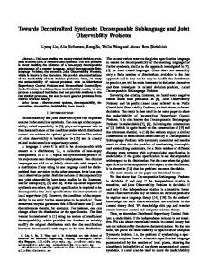
different initial conditions. The ballistic coefficient is variable, using the Allen oscillatory model which describes the oscillations of the incidence angle. The estimation is made using a random walk model. One particular difficulty was the correct dimensioning of the dynamic noise of this very random walk. We show that we can take it as the upper envelope of the derivative of the ballistic coefficient 3 versus time. Then we study the filters robustness versus the knowledge level of the true dynamic noise. This article has a two part structure. In the first part we study the FIM in a two dimensional simplification of dynamics with a constant 3. In the second part, we Figure 1: Two dimension reduction. compare in a general case of dynamics and 3 parameter the performance of EKF and particle filter with PCRB. We give a robustness analysis of the algorithms. Let r(t) be the range versus time. Using this expression 3 versus altitude, it is possible to obtain an exact 2 Local study of the PCRB by formula versus time, e.g. v[y(t)] by substituting
the Fisher Information Matrix
In this section, we will show that the observability is proportional to the object's acceleration. We start with the description of a 2D model that will be used to find analytical bounds.
2.1
Two dimension model
2.1.1 Notations and definitions Let A be the object cross-section, C its drag coefficient and m its mass. We note 3 the ballistic coefficient. The ballistic coefficient is the product CA and is expressed in m2.kg-'. We note go =-9.8m.s-2, the gravitational acceleration. We note alt the altitude; alt = y in the coordinate system of figure 1. The atmospheric density is given by: = 7000 and p(alt) = poexp{ (a"t) cp }kg.m3 with cp po= 1.2kg.m-3. 2.1.2 The two-dimensional reduction Let us deal with a classical two-dimensional reduction of the ballistic dynamics. We have represented on figure 1 a two dimension reduction of the problem. Let y be the constant re-entry angle, and vx, vy the two components of the speed. The differential equations of the reduction of dimension two are the following:
y(t) = sin(Oo)r(to) -
v[y(r)]sin(-y)dr
(4)
ft'
in equation (3). Then v[y(r)]dr is a solution of a differential equation. It is also possible to obtain - close to the initial condition - an approximation using the Taylor development of altitude as a function of time given in equation (5),
y(t) sin(Oo)r(to) - sin(-y)(t - to)v[y(to)]) (5) 2.1.4 Expression of range In the system we have two angles, -y (the re-entry angle) and ( (the angle between the re-entry path and the initial line of sight 0(0).) We want to evaluate the FIM for a radar observing range information and estimating r, v, 1 (It is possible to obtain the FIM if the radar estimates also 0, but here we suppose that 0,-y are estimated separately using bearing information). Let us note v[y(t)] the speed along the re-entry axis, and ( = 7r- . v[y(t)] is decomposed into two parts: The projection along the initial line of sight and the angular or orthogonal part: -
v,(t) =v[y(t)] cos(() v,(t) =v[y(t)] sin(()
(6) C is used to have a negative cosinus for the radial part of the speed vector. - cos(-y)-3.p(y)v2 (1) Vly = go + sin(,y)-1.p(y)v2, 2 2 We note r,(t) the projection of the radius along the Note that if go is neglected compared to dynamic pres- initial line of sight, ra(t) its orthogonal part. We suppose rr(t) >> rX,(t) . If we use the relasure 13pv2, as suggested in Allen's article [9], then tion VA2 + B2 A+ valid for real numbers 1 2 such as A the versus time r(t) B, range >> (2) + ra(t)2 is given by: 2 2.1.3 Expression of the speed versus altitude ) 2)/ ((r(to) + tvr)2 (It Allen finds the following solution of (1) in [9], by r(t) considering a constant -y angle and neglecting gravity forces compared to drag forces: r(to) + t Vrdr + (1/2) (t to ~~~(r(to) + f"t t vdrd) (3) v(y) =v[y(to)]exp(- 2sin(Y) pocpe Cp). 198 ,
VFrr(t)2
=
Authorized licensed use limited to: UR Rennes. Downloaded on July 16, 2009 at 06:34 from IEEE Xplore. Restrictions apply.
2.2 FIM determinant calculation Let us suppose a range-only observation function. 2.2.1 Definition of the FIM Let M be the observation function gradient along the trajectory: Mt=_
( Or(to)' ar(t) Ov[y(to)}' Or(t) 7r(t)N')(7
'(9
The consequence is the simple expression of the FIM determinant:
det(FIM(t.,t,))= a6r
O
det(MtP,Mt,,Mtr)2
= R(k)det(f2(to)). with R(k)- > P(tp-to, tq-to, tr- to)2 p
Expansion of the FIM around successive step and let Nt Mt, with ar the range measurement standard deviation. In a range-only measurement sys- of time. tem, the Fisher Information Matrix (FIM) is: The highly non-linear dynamics are leading to a S=tk S=tk I error in the Taylor approximation of formula growing MsIM FIM(to,tk) E NsN'8 if all terms are computed based on the matrix 10, r s=to s=to t , at the initial instant to. det(M, dM, z Then we can decompose the determinant to compute with Z = [Nto0 Nt, I... INtk ] the matrix whose each it based on Taylor expansions (10) evaluated around column is the vector Nt from t = to to t = tk. different intants to,- ,tk. The decomposition is as follows: 2.2.2 The Cauchy-Binet formula 1 If we want to compute the determinant det(FIM(to,tk = (6 det(Mtp,mtq,mt,)2 det(FIM(tO ,tk) ) = det(ZZ'), we have the followO
d2M)(to)
z
-
d2M [1(t [M,dM Q(t)~~ [M ~~ t) t4() M,(l) Expansion of the FIM around to. Let P(a, b, c) be:
(q)
M(2)](9)
+ 'Pi2
2)
av[y(t)]
(10)
Mt
Indeed, we have
av[y(t)]
d av[y](t) dt 9r(to) d av[y](t) dt 9v[y(to)] d 9v[y](t) dt 03(to) with dt)
M)P(tp, tq tr).det(i(to)).
I
t - to. By equation 10 we obtain:
Mtp A Mtq A Mtr
tq-rqr Mto M(2 + Mto A Mtol) A Mto2) 2
'A
(1) AMt0 A Mt A M('A) 2 +pt ~ AMt
+tPr + .2r
+.2
to
0
M to
++
r
r
2 2
A
(tol)
A
M2) AMto AAM(1)2 +to 2'2M to toA2)A
P(tp, tq tr)Mto A MA(l) to0 A M2to
M2 to
A
to
sin(Oo)
O
sin(a) v[y(t)]
av[y(to)I
det(Mtp , Mtq Mt,) = Mt A Mtq A Mt,. Let us note ti
(t
ar(to)
For (x,y,z) E R3, let w(x,y,z) = x/AyAz be a multilinear antisymmetric 3-form, an element of A 3(R3). Then
det(Mtp,Mt
P(tp tq,0,tr -tq
2.2.4 Computation of the matrix Q To compute the matrix Ql we will need some approximations. Using the system of exact equations (3) and (4), we show in the lemma 1, given in appendix, the following approximations of equations (11,12,13,14,15).
b2c a2b a2c 2 ac2 P(a, b, c) =-b2 + ab2 ++2 2 Let us note ti t - to. Let us suppose valid the Taylor expansion (see [10]):
Mti = Mto + t M
p
(12)
v[y(to)] I.
I
=
-
t)sin(Oo) sin(ay)
(11)
,
(13)
e(t) 0O
(14)
1 22p(t)v2
(15)
-
d3nffily v1ff
(16)
These approximations are valid if e(t) is small w.r.t. 1, a reasonable hypothesis. Indeed in our application v
Mp) A and ( (t) We ) Mto c.103M.s-1,3 also suppose that1.10-4m2.kg1, y is "big enough" too avoid singular sigua +values. To have an idea of p values, p = 1.10-4 at M1) 2.10-3 at 45 km of altitude to A Mt 65 km of altitude, p 0and p = 1.2 at altitude zero. We have the following property: 199
Authorized licensed use limited to: UR Rennes. Downloaded on July 16, 2009 at 06:34 from IEEE Xplore. Restrictions apply.
Property 1 Let us suppose valid the approximations of equation (11,12,13,14,15), and rr(t) >> ra(t). Then Q(t) is triangular and Q (t) 2,2] (t) l[3,3] (t) 1) det(Q(t)) ll1, 2) If the dynamic has no orthogonal part (E,0), -
if we remark that xx
8,Ixx
0, xx
0 (because
X is supposed much bigger than Y). Hence the information about non-radial component is proportional to the variation of 0, multiplied by the first (a8o-) and second (a3(o) ) integral of 'a
Vr 1 2 vr[(t) (t) 2.3 Computation of the CRB of coeffidet(&Z(t)) Vrv[y(to)1 2-p(t)v2 v[y(to)] 0 cient d Let us compute the CRB for the coefficient /3 in Proof: Let us set X r(to) + ftq v,dT, Y = oVadr. range only case. With a dynamic with no orthogonal 1) Q[1,2] By lemma 2 equation (34) and approxima-
part ((= 0). Other cases can be derived easily. We suppose the time divided into periods d Or IOY Va We suppose the existence of a [to, t2, ... , tkj. X dt ar(to) ar(to) first period t-1. The matrix FO FIM(t-1,t 1) Let us note represents a priori information. and But Or(to)(t) f Qr(torT)dr (orr ioa, ug) the a priori errors on r, v, /3. We 9Y vX ~0 hence Q[1,2J 0can suppose the matrix FO diagonal with &r(to) X ~ ~ 2) Q[1,3] By the lemma 2 equation (35) and approxi- FO[l,l] , FO[2,2] ,(a)2 FO[3,31 (_)2 The FIM expression is then: mations of equation (13), we have FIM(t,tk) = FO + FIM(totk) d2 ar aY ia R1X3 Wdt2 ar(to) ar(to) X The CRBQ of the coefficient 3 is the term (3,3) in the inverse matrix FIM(t_ ,tk). Let A be the (2,2) matrix hence f[1,3] °. extracted from FIM(t_1 )k), excluding the last column 3) Q[2,31 By the lemma 2 equation (35) and approxi- and last line. Using the well known property of inverse mations of equation (14), we have matrix we obtain: d2 ar aY va 1 CRBfl 0[2,3] dt2 aV[y(to)] X det(FIM(t_ l,tk)) .e()
tions of equation (11), we have
=
fftoE(-r)dr
=
I
1
1
OV[y(to)]
ButBt
ay () ,_t) av[y(to)]
-
ava ())dT ftoft v[Y(to)](T
d-r < sin ).(t -to) because v(to) > v(t) and 9v vo)IX 0 henceQ[2,31 04) Let us now compute the diagonal terms. By the lemma 2 equation (33) and approximation of equation (11) we obtain
sin(() g0Y
*t I
tf Vr(8)
ds = X(ti)-Xto) from equation (17) and (18). Using the determinant multi-linearity we obtain: k f2 1 Er1to fsgs det(A) = det ( ,a)7 +
ES=OJ
y
c(T)sin(()X dr.
1+ Ek=O 9s
Es=o fsgs
E(T)cos(C)dT
O= (t0) 1 + +
The matrix A can easily be obtained from the definition of the FIM (equation (8)) and from the value and9r gi 1 &a(ti) off2 1 ar(ti)
(17)
(a('J*av
O
s=O0
r~(~)2
+
)
(*)2) (UV)
To finish the computation, we just divide the two By the lemma 2 equation (34) and approximation of determinants, and take into account the initial knowlequation (12) we obtain edge. And because det(FIM(/31 tk)). (det(FO)1/3 + det(FIM(tO,tk) )1/3)3 Y Or d Va Vr obtain: We dt Ov ICRBf(tk)I < By the lemma 2 equation (35) and approximation of det(A) equation (15) we obtain + (~ Z 2p(tq)V2)2)1/3)1 S
[y(to)]
v[y(to)I Xv1t18)
Authorized licensed use limited to: UR Rennes. Downloaded on July 16, 2009 at 06:34 from IEEE Xplore. Restrictions apply.
Dynamic X = V(X), X = (X,Y,z,vx,vy,vz, 3)': vx Vy
x
Vz
(20)
Gx + 2x + 2fQvy-q3 vz~~~ Gy +Q2y _2QVX q/3y Gz - q/3
vx vz
d;3
0
with q = field Gx
-
i
1pllvllj, p = poexp{Xi gR
Xi
} and gravity
X,Y'aZ
The coefficient q = pIIvIl2 is the dynamic pressure. in function of Note that this model restricted to the equator, with z = vz = 0 is of dimension two, hence the analysis of the previous section is valid. The discretization of this model is used in the PCRB algorithm, in the particle 3 PCRB of the general model filter and in the EKF. We give this discretization in In RV tracking, the aim is to be able to estimate the subsection 3.1.3. object's position, speed and ballistic coefficient, using In our study the ballistic coefficient depends on altion one hand a priori dynamic and measurement model, tude. To equation (20), we thus put out =3 0, and we on the other hand radar observations. Finding a good simulation model reveals high complex- use the 3(alt) profile versus altitude, given on figure 3 ity, for two reasons: the first reason is the very high (details are given in [6]). level of dynamic non-linearity. The second reason is 3.1.2 A priori dynamic model the existence of non-deterministic parameters like the In this section, we describe the dynamic model ballistic coefficient, which is the product of the object the estimator supposes. It is called an a priori cross-section by the drag divided by the mass. The evolution versus time of the drag coefficient depends model. In the model, the differences observed between on the incidence angle. Allen [6] proved the very high measurements and the a priori model will be modeled variability of the incidence angle for a RV, inducing the by an additive dynamic noise on the coefficient / after same level of variability for the ballistic coefficient. In discretization. If the continuous a priori model of /3 is the simulations, we will use either a constant ballistic / = 0, its discretization gives, by adding an additive profile as a simplification and a reference, or a complex dynamic noise vuf: ,B(k + 1) /3(k) + v (k).(The noise sequence v/(k) is supposed white and gaussian). This Allen profile. Finding a good a priori dynamical model is a complex is a random walk model. task too. Like in [3] and [5] , it is possible to suppose only a random walk model for the ballistic coefficient. 3.1.3 Dynamical model discretization First we describe the simulation models in subsection Let At be the step of the filtering algorithm. 3.1.1, then we give the a priori model used in the trackWe suppose discrete time instants, indexed by k, ing and PCRB algorithms in subsection 3.1.2. (tl, t2, * , tk), such as tk+1 = tk + At. We will use the notation x(k) = X(tk),x(k + 1) = X(tk + At) for each state coordinate x. 3.1 Modeling The most direct discretization consists in a finite 3.1.1 Dynamic model for trajectory simuladifference. If we write equation (20) as: tions X V(X) we obtain: We suppose now an earth-centered coordinate system (ECF, see [3]) . We note Re the earth radius. X(tk + At) f(X(tk)) X(tk) + AtV(X(tk)) We note alt the altitude; alt _ Vx2 + y2 + z2 Re in ECF. We note Q the earth rotation speed, expressed For our estimation algorithms, we should add a in rad.s-1. We describe the deterministic dynamical dynamic noise. Thus we write a model with noise: models that we use to generate the trajectories of our X(tk + At) f(X(tk)) + V(tk) V(tk) Q(tk) We may write the model more simply, as follows: simulations.
Figure 2: The the periods
error
graph
V/CRB(/3)
The deterministic trajectory of the object with a constant / follows the differential equations given by:
X(k + 1) = f (X(k)) + v(k) v(k)
,
Q(k)
Q(k) is the Gaussian dynamic noise covariance matrix.
201
Authorized licensed use limited to: UR Rennes. Downloaded on July 16, 2009 at 06:34 from IEEE Xplore. Restrictions apply.
Measurement models Our radar model gives measurement in range d and angular measurement - the direct cosines (a, p, 77). Using a coordinate transformation matrix Mr, and with a radar located on earth with coordinates (xr, Yr, Zr), we obtain the measurements vector h(X) 3.1.4
h(X) = (ju,
q,
d)' with
*(x(kMl d
y(k) - yr, z(k) - Zr) + (v;(k), vr,(k), vd(k))' The measurement noise sequence (v,"(k), v,,(k), vd(k))' (a' 8)' -
ia
I
- xr,
is supposed white and gaussian and has a standard deviation for each coordinate, such as o-,= a,1 = 3.5 10-5, and ad = 1 m, like in [3]. The radar is placed on the equator at longitude zero.
3.2
I.-
Comparison between PCRB and filters, Robustness of the filters
We will study the performance of the EKF and of particle filters. These filters are compared with an algorithm establishing the maximum performance that can be reached by any filter. This is equivalent to find the lower bound of the empirical state covariance. The lower bound is called the a posteriori Cramer Rao Bound [4]. In this section, we compare the PCRB with particle filter and EKF. The particle filter is the same as the filter described in [7] and [3], with 10000 particles. We start with a constant /, then we use a variable 3, following the Allen oscillatory model. The initial vector (x, y, z, vx, vs, v.) is set to (6485921.9; -256897.4; 1.2 x lo5; -2627.6; 6271.8; 0). The initial altitude is 120km, the period is dt = 0.5s, and the intense braking phase starts at 60km, i.e. 45. 3.2.1 Comparisons between PCRB and filters During the experiences realized on PCRB and EKF filters, we observed the necessity of a correct dimensioning on the coefficient ,3. Let us show how it can be done. The ,3 dynamic can be described by
I
.-
- - 1. ...- ..
D- I-- ..
I
a
..
ins S__
-
_1 -1
.... .o .(m)
Figure 3: the coefficient : versus altitude and its derivative known d, - d dr dr On figure 3, we show on the left the derivative d: computed with the ballistic coefficient model we have used. One should notice that we took a big enough envelope, then overestimated the dynamic noise. This will imply an over-evaluation of the PCRB during the simulations. In order to solve the problem, we will show in the simulations the evaluation of the PCRB with the exact envelope of the oscillations.
Comparison between particle filter and EKF, Robustness We present the results obtained with a well known dynamic noise on figure 4. If the dynamic noise is under-evaluated, we obtain the figure 5. Interpretation of the results
a) Perfectly evaluated dynamic noise. On figure 4, we show the comparisons between particle and EKF filter, RMS error and PCRB. The finite variation theorem gives: The dynamic noise for the black, blue and red graphs is the dynamic noise given by the large envelope of max < +At) dO(c)At (21) 1/3(tk 3(k)l figure 3. EE[tk,tk+at1 dt The dynamic noise for the green graph is the exact Hence envelope of the graph of figure 3. The best estimation of the bound is done when the -2= EI/3(tk + At) -:(k)|12 < mee[taxtt] dt dynamic noise is evaluated with the exact envelope. The behaviour of the EKF is exactly the same as Let us note r the altitude, and e* the value of c which the case of a set /3, the EKF remains stuck on the realizes the maximum of (21). It appears clearly that initial value until the gain becomes big enough. This we can choose: aV = dlt3(e*)At Because /3 is expressed explains why the EKF error is getting through PCRB with altitude, we will take a>,, helped by the chain in the first part of the trajectory. More precisely, let rule, equals to : a,, d (E*)dOAt If we suppose us refer to figure 3. The first estimate of 3 is the value 202
/3(tk + At) =/3(k) + v(k), v(k) N(0, a^) -
Authorized licensed use limited to: UR Rennes. Downloaded on July 16, 2009 at 06:34 from IEEE Xplore. Restrictions apply.
-ur Compoa-iso-saour
(bu-nn connoinc- sur 1o brult d- B)
PARTICULAIRE EKIF
A
A
AA
b-ft dy.n.ur.1u upti.mu nPCRB, PCRB
E
i. u1
Figure 4: Error on the coefficient ,3 Compsrloions -rrour sur p (bruit do
sous o ti-n.)
PARTICULtIRE EKF PCRB PC R.immtr
Pmi-i1u mptum,ui
The PCRB shows that the ballistic coefficient is not immediatly observable. The evolution of the estimation error unfolds in two steps. First, periods where the re-entry is not really started, and where the error is increasing. Second, the RV reaches dense atmospheric layer, leading to a fast decrease of the error. This decrease was announced by the analytic FIM study. During the comparison study between PCRB and tracking algorithm, it appeared that the knowledge of the variations of 3 is fundamental to obtain the correct dynamic noise dimension. This knowledge is ideal if we know the object, its initial incidence angle and the drag dependancy on the initial angle. If this knowledge is imperfect, the particle filter gives a better robustness than the EKF. If the knowledge is perfect, the EKF has excellent performance. The PCRB shows precisely the instants of the estimation algorithm optimality, and the instants of possible improvement.
Lemma 1 The approximations given in equations (11,12,12,14,15) are valid. a) Equations (11) and (12) Let us recall the dynamical system: 1 Figure 5: Error on the coefficient /
Y
v[y(t)]
=
v(to)exp(- 2 i(Y)pocpee cP ). (22)
y(t)
=
sin(Oo)r(to) -
rt
v[y(r)]sin(-y)dr(23)
Let us differentiate equation (22), we obtain on the very right on the graph, added to a noise. This O3v[y(t)] _ p(t)/v[y(t)] Oy(t) e(t) Oy(t) (24) particular evolution of the coefficient produces the Or(to) Or(to) 2sin(-y) sin(y) ar(to) following event: if the estimate remains blocked, the Ov[y(t)] p(t)/v[y(t)] ay(t) + v[y(t)] error increases and then becomes exactly the same as the beginning around the altitude of 75 km. 2sin('y) Ov[y(tO)] V[y(to)] a3v[y(to)] On figure 4, the PCRB graphs obtained with large e(t) Oy(t) + v[y(t)] (25) and exact envelopes are the same. sin(-y) av[y(tO)] v[y(to)] Eventually, we may say that when the dynamic noise is well evaluated, the particle and EKF filters are If we differentiate equations (23), we obtain equivalent. 6y(t) sin(Oo)- t v(-() sin(-y)dr (26) ar(to) ito r(to) b) Under-evaluated dynamic noise. It av (r) By under-evaluated dynamic noise, we mean a dynamic t9y(t) (27) &v[y(to)] noise on /3 equal to the dynamic noise given by the large -0 envelope of the 3 oscillations, divided by ten. Given If we substitute equation (26) in (24) and equation (27) the simulation results of figure 4, it is clear that the in (25), we obtain: particle filter's robustness is higher than the EKF's. When the dynamic noise is not well evaluated, Kalman Ov[y(t)] e(t) ft v[y(T)] gains are very far from the optimal gains. The particle afr(to) sitn(y) sin()s ) to 23r(to) filter estimates the value of 3 earlier than EKF. v[y(t)] av[y(t)] _ (t) J ft av[y(r)] si-y) dr ± v[y(t)I _sin(a sinQy)~ v [y(to)] si( av[y(to)] V[IVO]
8t,v[y(to )]sinlQy)dT
e(t)in(o
4 Conclusion
The FIM, the CRB inverse, says that in the observ- or, by setting S = ft.t ability is proportional to the object's acceleration. UsS' = ing the Allen solution, we gave an analytical approximation of the CRB of the ballistic coefficient /. This analytical function gives a two-step evolution and thus T' = a two-step observability, these steps are related to the dynamical pressure brutal evolution versus time . S(0) = 203
ftJto 9v[5(T)] dr. ov[y(o)] v[y(to)] Or(to) dr and T
E() sin(O) -e(t)S
sin Q.Y)
-e(t)T +
v[IY(to)]
0, T(0) = 0
Authorized licensed use limited to: UR Rennes. Downloaded on July 16, 2009 at 06:34 from IEEE Xplore. Restrictions apply.
(28) (29)
(30)
This can be solved to give (just differentiate to verify): _e
t
'E(w)dw
E(s)dsI t
T= e-E(s)ds et
t
e
c(s)
Proof: For the first part, it is a simple application of differential calculus. For the second part, we just have (31) to remark that:
(
ftso
v[(tO)ds (32)
dt 1
Now we substitute equation (31) and (32) in (28) and
(29): av[y(t)] I_I ar(to)
)s]l
V
[Y(to)] (t). 0 [^[[(t ))] +c
&MOI
[5] A. Farina, B.Ristic, D. Benvenuti Tracking a Ballistic Target, comparison of Several nonlinear Filters IEEE Trans. on aerospace and electronic systems July 2002 Vol 38 number 3.
[6] H. Jullian Allen, Murray Tobak Dynamic stability of vehicles ascending or descending paths through the atmosphere NACA Technical note 4275 july 1958
-
[7] B. Ristic, S. Arulampalam, J. Mc Carthy Target Motion Analysis Using Range-only Measurements: Algorithms, Performance and Application to INGARA ISAR Data DSTO-TR-1095, January
Let r = X + y2 such as X = r(to) t+fj Vrdr,Y f= Vadr. then 1
and d ar
O3Vr
9Y d(-) avr x
Tp +ap
dtap
OYY
dt
-
horai Posterior Cramer-Rao Bounds for DisreteTime Nonlinear filtering IEEE Transaction on signal processing vol 46, no 5 may 1998
hence a 1p 1212 PX d Ov pcp 2 2 vsin oi,3 dt (9, But cp and v are of the same order. cp = 7000 and v = c x lOOOm.s-1. This proves the formula (15) Lemma 2 Let p be a real parameter, like r(to),v[y(to)]
ap ±Op X
x
[4] Petr Tichavsky, Carlos H. Muravchink, Aye Ne-
(-2.n pcp)
OX
Vr
Va
[3] Pierre Minvielle Tracking a ballistic Re-entry Vehicle with a Sequential Monte- Carlo Filter 2002 IEEE Aerospace conference March 9-16 , 2002.
c) Equation (15) Using equation (22), one can obtain: 1 Ov
Or ap
d( t ) dt
Vr
X2
Bucy Filters for Radar tracking and Identification Proceedings of the 1991 IEEE National radar conference, IEEE Aerospace and Electronic Systems Society, 1991, pp. 127-131
) [y(t) I -d Ov[y(t)] 2ct)3v C ar(to) dt Or(to) ar(to) d O3v[y(t)] ai4[y(t)] 2 Ov[y(t)] dt Ov[y(to)] av[y(to)] 2tVO[y(to)] and the approximations of equations (11) and (12) give the result.
Letr~~~~~~~~~~~~~~
X
X
[2] P.J. Costa and W.H. Moore, Extended Kalman-
b) Equations (13) and (14) To prove formula (13), and (14), one should notice that v= p(t)/3v2 and then
or,3.
V,
Va
dt
A Track Filter for reentry Objects with Uncertain drag IEEE Transactions on Aerospace and Electronic systems, Vol 35, n2, April, 1999
ds
This proves formula (11) and (12).
X
V X2
d(d)
[1] G.P. Cardillo, A. V. Mrstick and T. Plambeck
ds
av[y( av[y(Ito)]
dQy)
X dt
Y X3
References
d .E(t)sin(GO) +etft e(s)sin(Oo) v+[ (t) i
S'<
a x2-
d(d )
E(w)dw V[y(S)]
ft.
1( Y)2
22 X
2001
X
[8] H. Jullian Allen, Motion of a ballistic missile
a(p
Y aVa 1 av Y +- -~~1O -=(Y)2 X ap 2 ap X
Y d(X) AX dt ap if X >> Y then d Or Ovr + OY Va + Y ava 1 avr (34) dtAp Etp dp X X -p 2 Op X and d2 ar 9i)r + Ova Va OY ia Va O9va Y O9i)a Op pX OpXXOpXOp
[9] H. Jullian Allen, A.J. Eggers, Jr. A study of the motion and aerodynamic heating of ballistic missiles entering the earth's atmosphere at high supersonic speeds NACA Technical note 1381
-
(.Y)2
an-
gularly misaligned with the flight path upon entering the atmosphere and its effect upon aerodynamic heating, aerodynamic loads, and miss distance NACA Technical note 4048 october 1957
[10] Jean-Pierre Lecadre, Properties of estimability criteria for target motion analysis, IEE proceedings in Radar, Sonar Navigation No 2, April 1998
204
Authorized licensed use limited to: UR Rennes. Downloaded on July 16, 2009 at 06:34 from IEEE Xplore. Restrictions apply.
°