PHYSICAL REVIEW B 77, 144424 共2008兲
Rate of magnetization reversal due to nucleation of soliton-antisoliton pairs at point-like defects Peter N. Loxley School of Physics, The University of Sydney, New South Wales 2006, Australia 共Received 10 October 2007; revised manuscript received 31 March 2008; published 23 April 2008兲 The rate of magnetization reversal due to the nucleation of soliton-antisoliton pairs at point-like defects is found for a uniaxial ferromagnet in an applied magnetic field. Point-like defects are considered as local variations in the magnetic anisotropy over a length scale smaller than the domain-wall width. A weak magnetic field applied along the easy axis causes the magnetization to become metastable, and the lowest activation barrier for reversal involves the nucleation of a soliton-antisoliton pair pinned to a point-like defect. Formulas are derived for the activation energy and field of reversal, and the reversal-rate prefactor is calculated using Langer’s theory for the decay of a metastable state. As the applied field tends to zero, the lowest activation energy is found to be exactly half that of an unpinned soliton-antisoliton pair, and results from the formation of a spatially nonuniform metastable state when the defect strength become large. The smallest field of reversal is exactly half of the anisotropy field. The reversal-rate prefactor is found to increase with the number of point-like defects but decreases with increase in the defect strength due to a decrease in the activation entropy when translational symmetry is broken by the point-like defects, and soliton-antisoliton pairs become more strongly localized to the pinning sites. DOI: 10.1103/PhysRevB.77.144424
PACS number共s兲: 75.60.Jk, 64.60.Q⫺, 64.60.My, 05.45.Yv
I. INTRODUCTION
Thermal stability and the decay of metastable states have been widely studied since the pioneering work of Van’t Hoff and Arrhenius.1 Detailed theories of thermally activated magnetization reversal were originally proposed for singledomain ferromagnetic particles.2,3 However, recent interest in multidomain ferromagnets such as elongated particles and nanowires, exchange springs, and coupled magnetic grains has led to new theories and new predictions for rates of thermally activated reversal.4–8 During the reversal of a single-domain ferromagnetic particle, the magnetization is assumed to rotate coherently. This is no longer true for effectively one-dimensional 共1D兲 ferromagnets, where reversal can take place via the nucleation of soliton-antisoliton pairs.4,5 This typically takes place as follows: Initially, the magnetization is uniformly aligned along a particular anisotropy axis but becomes metastable when a weak magnetic field is applied in the opposite direction to the magnetization, that is, it remains stable to small thermal fluctuations which occur frequently but becomes unstable to the less frequent larger fluctuations. The magnetic anisotropy is generally sufficient to stabilize the magnetization when small fluctuations are present. However, a large fluctuation may create a region of partially reversed magnetization which forms a nucleus of critical size. Following the formation of a nucleus of critical size given by a soliton-antisoliton pair, the soliton and antisoliton are driven apart by the applied field, and the magnetization reverses direction. Solitons as fundamental excitations in 1D magnets is not a new concept, and much work has previously been done on soliton statistical mechanics and nonlinear dynamics following the work of Bloch, Döring, Enz, and Walker.9–14 However, recent experimental progress in the preparation and characterization of ferromagnetic nanowires,15–19 including multilayered nanowires and nanowires with controlled defects, has generated particular interest in the reversal mechanisms and 1098-0121/2008/77共14兲/144424共14兲
switching rates of 1D magnetic systems.4–7,20–26 In many realistic situations, it is known that nucleation occurs at a nonuniformity or defect—such as an irregularity in a sample. Such defects supposedly lower the activation energy for nucleation, allowing it to occur more frequently. In magnetic systems, defects may include nonuniformities in the magnetic anisotropy and exchange,6,7 or local deviations from an otherwise uniform geometry.27 Reversal due to nucleation at defects presents some conceptual difficulties. For example, a defect which lowers the activation energy for nucleation usually favors domain-wall pinning over domainwall propagation: the opposite of what is required for reversal to take place. How defects modify the nucleus of critical size and the metastable state is also largely unknown. Another consideration is the probability of nucleation at a defect. There are usually far fewer nucleation sites available for nucleation at a defect than for nucleation elsewhere in a sample. The purpose of this paper is to carry out a theoretical investigation of thermally activated magnetization reversal due to nucleation at defects. The type of defects considered includes local variations in the magnetic anisotropy over a length scale smaller than the domain-wall width—so-called point-like defects. Activated reversal due to defects larger than the domain-wall width has previously been treated in Refs. 6 and 7. A general model of a 1D uniaxial ferromagnet in an applied magnetic field is employed to calculate the rate of reversal using Langer’s theory for the rate of decay of a metastable state.28,29 Although 1D magnetic systems are specifically treated, the model is general enough to include other 1D systems which obey a time-independent double sineGordon equation. The rate of thermally activated reversal can be described using the well-known Van’t Hoff–Arrhenius law: I = I 0e −Ea ,
共1兲
where Ea is the activation energy, and is given by the height of the lowest energy barrier separating a metastable magne-
144424-1
©2008 The American Physical Society
PHYSICAL REVIEW B 77, 144424 共2008兲
PETER N. LOXLEY
tization state from the fully reversed state,  = 1 / kBT, and I0 is the reversal-rate prefactor and depends on the dynamics of crossing the activation barrier, as well as on the activation entropy—the entropy difference between the activated and metastable states.1 The exponential in Eq. 共1兲 implies thermal activation takes place over a much larger time scale than the time scales in I0 characterizing the magnetization dynamics. Previous theories for nucleation at point-like defects have concentrated on calculating Ea using the sine-Gordon model,30 and Ea and I0 using a reaction-diffusion equation with piecewise-linear nonlinearity.31 Neither of these treatments is adequate for addressing the questions posed here. The first treatment does not attempt to find I0, and neither treatment considers the double sine-Gordon model—which is necessary for describing a ferromagnet in an applied magnetic field. In this work, mathematical analysis is used to derive expressions for Ea and I0 for a 1D uniaxial ferromagnet in an applied magnetic field. The structure of this paper consists of two parts. In Secs. II and III, the model is introduced, and a reversal mechanism is proposed from consideration of the minima and saddle points of the relevant energy function. A critical defect strength is identified—above which the metastable state may become spatially nonuniform—and formulas are derived for Ea and the field of reversal Hrev above and below the critical defect strength. In Sec. IV, a formula is derived for I0 below the critical defect strength as the applied field tends to zero. This allows for a reasonably straightforward understanding of how the presence of point-like defects can modify I0. A summary and discussion of the main results is given in Sec. V.
H
K2
K1
K2
FIG. 1. A 1D uniaxial ferromagnet resulting from a cylindrical geometry with d ⬍ ␦ex. The easy axis lies along the longitudinal axis, and a magnetic field is applied along the easy axis. A pointlike defect represents a local reduction in the strength of magnetic anisotropy 共K1 ⬍ K2兲, or a local misalignment in the anisotropy direction 共K1 ⬍ 0兲. The sequence of arrows represents a metastable magnetization state.
␦ex, where ␦ex = 冑A / 0M s2 is the magnetic exchange length.5 Below this critical length, the cost in exchange energy for m to deviate from a uniform configuration outweighs the possible reduction in energy from the demagnetizing field. One possibility for a 1D uniaxial ferromagnet therefore consists of a cylindrical geometry with d ⬍ ␦ex, as shown in Fig. 1. Values of ␦ex range between 5 and 10 nm for common ferromagnetic materials such as Co, Ni, and Fe.32 Defects in the magnetic anisotropy are taken into account by allowing K共x兲 in Eq. 共2兲 to vary with x. If Ld is the defect width, a point-like defect is assumed to satisfy Ld ⬍ ␦w, where ␦w is the characteristic domain-wall width. Provided that exchange coupling extends over the defect region, a point-like defect located at x = 0 can be approximated using K共x兲 = K − ⌬KLd␦共x兲,
II. MODEL
The magnetization is described by the unit vector m, and the energy of magnetic configurations of a 1D uniaxial ferromagnet of length L, and cross-section area Ar, is assumed to have the form
冕 冋冉 冊 L/2
E = Ar
dx A
−L/2
m x
2
册
− K共x兲m2x − 0M sHmx .
共2兲
The first term in Eq. 共2兲 follows from the classicalcontinuum limit of the exchange interaction between neighboring spins in the Heisenberg Hamiltonian, while the second and third terms describe the magnetic anisotropy and Zeeman energies due to an easy axis along the x axis and a magnetic field applied along the easy axis, respectively.13,14,32 The first term energetically favors uniform magnetization, the second term favors magnetization which points in either direction along the easy axis, while the last term breaks this symmetry so that one direction is favored over the other. A key assumption in applying Eq. 共2兲 to ferromagnetic materials is that the magnetization varies only along the longitudinal direction of a sample, and any transverse variation is assumed to be negligible. This 1D approximation is expected to hold whenever the transverse length is less than
共3兲
where ⌬K 艌 0 is the change in K due to the defect and ␦共x兲 is the Dirac delta function. In Fig. 1, K = K2 and ⌬K = K2 − K1 has been assumed. A defect leading to a reduction in the strength of magnetic anisotropy will satisfy K1 ⬍ K2, while a defect corresponding to a local misalignment in the anisotropy direction may have K1 ⬍ 0. The anisotropy constants include both crystalline and local magnetostatic effects.5 The magnetization is assumed to undergo dissipative dynamics according to the Landau-Lifshitz equation:
M ⌳␥ = − ␥M ⫻ Heff − M ⫻ 共M ⫻ Heff兲, t Ms
共4兲
where M = M sm, ␥ is the gyromagnetic ratio, and ⌳ is a dimensionless damping parameter.13,14,32 The first term in Eq. 共4兲 describes precession of the magnetization in an effective magnetic field given by Heff = −␦E / ␦M and conserves the energy. The second term is nonconservative and describes the relaxation of M toward Heff due to energy dissipation. The effect of thermal fluctuations could also be included in Eq. 共4兲 by adding an additional term to represent stochastic forces acting on the magnetization.4 Here, however, thermal fluctuations will be treated using the methods of statistical mechanics, as shown in Appendix A. The length, energy, and time scales of interest are the width ␦w and energy 2⌬w of a domain wall outside the
144424-2
PHYSICAL REVIEW B 77, 144424 共2008兲
RATE OF MAGNETIZATION REVERSAL DUE TO…
defect region and the characteristic time of magnetization precession in the anisotropy field outside the defect region, where
␦w =
冑
A , K
⌬w = 2Ar冑AK,
=
Ms . 2␥K
共5兲
The magnitude 兩m兩 is conserved by Eq. 共4兲, and the magnetization is most conveniently expressed in spherical-polar coordinates as m = 共sin cos , sin sin , cos 兲. In terms of spherical-polar coordinates and the characteristic length and energy scales defined in Eq. 共5兲, the energy expression given by Eq. 共2兲 becomes
冕 冋 再冉 冊 L/2
1 dx E= 2 −L/2
x
2
冉 冊冎
+ sin2 x
2
册
+ V − ␣␦共x兲Vd , 共6兲
sine-Gordon equation, and spatially uniform configurations satisfy V⬘共兲 = 0. When h = 0, two of the degenerate minima of V共兲 are given by = 0 and = and correspond to the magnetization pointing in either direction along the easy axis. When h ⬎ 0, the degeneracy is broken, and the minimum at = becomes metastable at nonzero temperature— thermal fluctuations eventually lead the system to the lower energy minimum at = 0. Spatially nonuniform configurations can be found for ␣ = 0 by integrating Eq. 共10兲 once using the integrating factor d / dx to yield
冉 冊
1 d 2 dx
V = Vd − h sin cos ,
sap = s 共7兲
and where a dimensionless defect strength ␣ and a dimensionless applied field h have been defined as Ld⌬K ␣= ␦ wK
h=
0 M sH . 2K
x − x0
␦s
共9兲
Mechanisms for thermally activated magnetization reversal involve configurations which are the minima and saddle points of Eq. 共6兲. Local minima of Eq. 共6兲 become metastable at nonzero temperature due to thermal fluctuations, and magnetization reversal involves crossing over the lowest saddle point in Eq. 共6兲 separating a local minimum from the global minimum. Following the identification of a critical defect strength, a reversal mechanism is proposed, and the corresponding activation energy and field of reversal are found. A. Energy minima and saddle points
Configurations which are minima, maxima, or saddle points of Eq. 共6兲 solve the corresponding Euler-Lagrange equations. The Euler-Lagrange equation for is solved by = / 2, and the Euler-Lagrange equation for then becomes
冊 冉
− R + s −
x − x0
␦s
冊
−R ,
共12兲
1
冑1 − h ,
sech2 R = h.
共13兲
The parameter 2R gives the distance separating the soliton and antisoliton as h → 0, while x0 is the position of the “center of mass” of the soliton-antisoliton pair. The value of x0 is arbitrary in a uniform system due to the underlying translational symmetry, while R is fixed by the applied field according to Eq. 共13兲. In any sequence of configurations which transform = into = 0, the soliton-antisoliton pair has the maximum energy. Relative to = , this energy is given by Esap = 4冑1 − h − 4h arcsech共冑h兲.
共14兲
For the biaxial ferromagnet considered in Ref. 4, Eq. 共14兲 represents the activation energy for reversal when no defects are present. Inclusion of a point-like defect implies ␣ ⫽ 0 in Eq. 共10兲. Integrating this equation from − to , and letting → 0, yields the following consistency condition:
冏 冏 冏 冏 d dx
−
x=0+
d dx
x=0−
= 兩 − ␣Vd⬘共兲兩x=0 .
共15兲
The simplest configuration satisfying Eq. 共15兲 has a continuous first derivative everywhere, and Eq. 共15兲 reduces to Vd⬘共兲 = 0 at x = 0. Upon using Vd from Eq. 共7兲, the nontrivial pinning solution is given by = / 2 at x = 0. The solution given by Eq. 共12兲 can be made to satisfy this by choosing x0 to be x0
␦s
共10兲
where V共兲 = −1 / 2 cos2 − h cos and Vd共兲 = −1 / 2 cos2 . When ␣ = 0, Eq. 共10兲 reduces to the time-independent double
共11兲
where s共y兲 = 2 arctan ey represents a single soliton, s共−y兲 represents an antisoliton, and
共8兲
III. REVERSAL MECHANISM AND ACTIVATION ENERGY
d 2 − 2 + V⬘共兲 − ␣␦共x兲Vd⬘共兲 = 0, dx
冉
␦s =
and
− V共兲 = C,
where C is an arbitrary constant of integration. In the limit as L → ⬁, integrating Eq. 共11兲 with C = 1 / 2 − h yields a bound soliton-antisoliton pair 共see Ref. 33兲:
where 1 Vd = − sin2 cos2 , 2
2
冉冑 冊
= ⫾ arccosh
1−h . h
共16兲
The configuration given by Eqs. 共12兲 and 共16兲 describes a pinned soliton-antisoliton pair: a soliton-antisoliton pair with either the soliton or the antisoliton centered at x = 0. This
144424-3
PHYSICAL REVIEW B 77, 144424 共2008兲
PETER N. LOXLEY
solution is valid for 0 艋 h 艋 1 / 2. The energy can be found using Eqs. 共6兲, 共12兲, and 共16兲 and relative to = is given by Epin = Esap − ␣/2.
0.4 h=0.5 0.2
F(cos φ0)
共17兲
The types of defect considered here satisfy ␣ ⬎ 0, so Epin ⬍ Esap, and the energy of a soliton-antisoliton pair decreases when it becomes pinned to a point-like defect. The simplest configuration satisfying Eq. 共15兲 with a discontinuous first derivative is one that is symmetric at the pinning site: 共−x兲 = 共x兲. Such a configuration can be constructed as
=
再
sap共x + x0兲, x ⬎ 0 sap共x − x0兲, x ⬍ 0,
冎
共18兲
where sap共x − x0兲 is given by Eq. 共12兲 and sap共x + x0兲 has the same form as Eq. 共12兲, but with x0 of the opposite sign. For this configuration, Eq. 共15兲 becomes 2d / dx = ⫾ ␣Vd⬘共兲 at x = 0. To write d / dx in terms of sap, the first integral given by Eq. 共11兲 and the boundary conditions satisfied by Eq. 共12兲 are used, yielding 共dsap / dx兲2 = 2V共sap兲 + 1 − 2h. Upon using this and the expressions for V and Vd, Eq. 共15兲 can be written as F共cos 0兲 = 0, where
冋 冉
F共m兲 ⬅ 共1 − m兲 1 −
␣ m 2
冊冉
1+
冊 册
␣ m − 2h 关1 + m兴, 2 共19兲
and 0 ⬅ 共x = 0兲 depends on the value of x0. This equation has four possible solutions for cos 0, each one corresponding to a different configuration of Eq. 共18兲. The = state is given by the cos 0 = −1 solution which always satisfies this equation 共a different choice of boundary conditions will yield a solution for the = 0 state兲. Classifying the behavior of Eq. 共19兲 at m = −1 allows critical values of the applied field and defect strength to be identified. Specifically, at m = −1, F⬘共m兲 = 0 when h = hcrit and F⬙共m兲 = 0 when ␣ = ␣crit, where hcrit = 1 −
冉冊
␣ 2 , 2
␣crit = 2/冑5 ⯝ 0.89.
共20兲
These critical values allow the metastable state to be properly quantified. It will be shown that = becomes unstable when h = hcrit. If ␣ ⬍ ␣crit, it then decays into the fully reversed state = 0. However, if ␣ ⬎ ␣crit, it will be shown that = decays into a new metastable state which is spatially nonuniform. A mechanism for reversal is now proposed. B. Reversal mechanism for ␣ ⬍ ␣crit
In the absence of defects, reversal of a 1D ferromagnet involves the nucleation of a soliton-antisoliton pair from a uniform metastable state,4 as outlined in Sec. I. However, the presence of one or more point-like defects leads to a saddlepoint configuration of lower energy. When h 艋 1 / 2, this is given by the pinned soliton-antisoliton pair from Eqs. 共12兲 and 共16兲. Upon reintroducing units into Eq. 共17兲, the energy required to nucleate a pinned soliton-antisoliton pair becomes
h=0.65
0 h=0.84
−0.2 −0.4 −0.6 −0.8 −1
−0.8
−0.6
−0.4
−0.2
0
cos φ0 FIG. 2. Graphical solution of F共cos 0兲 = 0 for ␣ ⬍ ␣crit. When ␣ = 0.8, the left-hand side of Eq. 共19兲 共solid兲 intersects zero 共dashed兲 twice between −1 艋 cos 0 艋 0 for 0.5艋 h ⬍ 0.84.
⌬Enuc = 2Ar冑AKEpin .
共21兲
This energy reaches a maximum value ⌬Enuc = 8Ar冑AK as h → 0 and ␣ → 0, which is the energy of two domain walls.32 When ␣ = ␣crit and h = 1 / 2, Eq. 共21兲 reaches its minimum value: ⌬Enuc ⯝ 1.24Ar冑AK, which is less than one-third the energy of one domain wall.32 Following the nucleation of a soliton-antisoliton pair, reversal takes place when the pair moves apart under the action of the applied field. However, it will be shown in Sec. IV B that one member of the pair remains pinned to a point-like defect if h ⬍ ␣ / 2. In this case, a soliton must become unpinned before reversal can be completed. From Eq. 共2兲, the maximum energy to unpin a soliton is ⌬Edp = Ar⌬KLd at zero applied field and results from the sudden increase in anisotropy at the center of the soliton when it is moved away from the defect region. When the applied field is nonzero, ⌬Edp will decrease due to the Zeeman energy contribution. Written in terms of ␣, this implies ⌬Edp 艋 Ar冑AK␣ .
共22兲
Comparing Eqs. 共21兲 and 共22兲, it is seen that ⌬Enuc ⬎ ⌬Edp when ␣ ⬍ ␣crit, so nucleation provides the rate-determining step for reversal. The activation energy for reversal is therefore given by Ea = ⌬Enuc .
共23兲
At h = 1 / 2, there is a smooth transition from the saddlepoint configuration given by the pinned soliton-antisoliton pair in Eqs. 共12兲 and 共16兲 to one given by Eq. 共18兲 with 0 = / 2. A graphical solution of F共cos 0兲 = 0 for ␣ ⬍ ␣crit and h 艋 hcrit is given in Fig. 2. At h = 1 / 2, the 0 = / 2 solution corresponds to the rightmost intersection of the solid curve with the dashed line in Fig. 2. When h ⬎ 1 / 2, this intersection moves toward the intersection at cos 0 = −1, until they eventually coalesce at hcrit = 0.84 when the slope of the solid curve goes to zero at cos 0 = −1. In this case, the saddlepoint configuration has merged with the = metastable state, which subsequently becomes unstable. The activation energy for reversal then vanishes, and reversal takes place spontaneously. After reintroducing units, the field of reversal is given by
144424-4
PHYSICAL REVIEW B 77, 144424 共2008兲
RATE OF MAGNETIZATION REVERSAL DUE TO… π
F(cos φ0)
φ(x)
h=0.35
0.3
h=0.5 0.1
0 −20
−10
0
10
π
φ(x) −0.8
−0.6
−0.4
−0.2
0
(b)
π/2 0 −20
−10
0
10
20
x
cos φ
π
φ(x)
0
FIG. 3. Graphical solution of F共cos 0兲 = 0 for ␣ ⬎ ␣crit. When ␣ = 1.8, the left-hand side of Eq. 共19兲 共solid兲 intersects zero 共dashed兲 three times between −1 艋 cos 0 艋 0 for 0.5艋 h ⬍ 0.61.
(c)
π/2 0 −20
−10
0
10
20
x π
共24兲
φ(x)
2K Hrev = h . 0M s crit
20
x
h=0.61
−0.1
−0.3 −1
(a)
π/2
0 −20
When ␣ = 0, Eq. 共24兲 reaches its maximum value Hrev = 2K / 0M s, which is just the anisotropy field,32 corresponding to the field of reversal when no defects are present. When ␣ = ␣crit, Eq. 共24兲 yields Hrev = 1.6K / 0M s, which is exactly 0.8 of the anisotropy field.
(d)
π/2 −10
0
10
20
x φ(x)
π
(e)
π/2 0 −20
−10
0
10
20
x
C. Reversal mechanism for ␣ ⬎ ␣crit
When ␣ ⬍ ␣crit, the uniform metastable state becomes unstable as the saddle-point configuration merges with = at h = hcrit. This is no longer possible when ␣ ⬎ ␣crit, and the uniform metastable state becomes unstable only after a nonuniform metastable state has been created. A graphical solution of F共cos 0兲 = 0 for ␣ ⬎ ␣crit and h ⬎ hcrit is shown in Fig. 3. When h = 0.35, there are two intersections in Fig. 3 as the local minimum moves away from cos 0 = −1, corresponding to two solutions of F共cos 0兲 = 0. When h = 1 / 2, there are three intersections in Fig. 3: the leftmost one giving the = configuration, the rightmost one recognized as the saddle-point configuration from Eq. 共18兲 with 0 = / 2 discussed previously, and the intermediate one giving a spatially nonuniform metastable configuration from Eq. 共18兲. Increasing h beyond h = 1 / 2 causes the intersections for the saddle point and nonuniform metastable configurations to move toward each other, until at h ⯝ 0.61 they coalesce. The activation energy for reversal then vanishes, and reversal takes place spontaneously. It is generally difficult to derive analytic expressions for the activation energy and field of reversal when ␣ ⬎ ␣crit. One exception is the limit ␣ → ⬁, where both quantities become independent of the defect strength. When h = 0, a solution of Eq. 共19兲 is given by cos 0 = −2 / ␣ for ␣ 艌 2. The corresponding configuration from Eq. 共18兲 is shown in Fig. 4共a兲 and was termed a “solitary dipole” in Ref. 30. The solitary dipole becomes metastable for infinitesimal h, and the saddle-point configuration shown in Fig. 4共b兲 is given by the pinned soliton-antisoliton pair from Eqs. 共12兲 and 共16兲. Both configurations have 0 = / 2 as ␣ → ⬁, so the only important difference between them is given by the dashed curve in Fig. 4共b兲. Since this dashed curve is exactly half a soliton-
FIG. 4. Reversal mechanism for ␣ → ⬁ and infinitesimal h. In 共a兲, a metastable configuration given by a solitary dipole is shown. In 共b兲, a saddle-point configuration given by a pinned solitonantisoliton pair differs from the solitary dipole by the dashed curve. Following nucleation, the soliton and antisoliton move apart 共arrow兲, leaving a metastable pinned soliton in 共c兲. In 共d兲, a second nucleation event completes reversal, leaving a stable solitary dipole in 共e兲.
antisoliton pair as h → 0 and since E = 兰dx共 / x兲2 on either side of the point-like defect from Eqs. 共6兲 and 共11兲, the energy to nucleate a pinned soliton-antisoliton pair from a metastable solitary dipole becomes ⌬Enuc = Esap / 2, or in the units of Sec. II, ⌬Enuc = 4Ar冑AK,
共25兲
which corresponds to the energy of one domain wall.32 Following nucleation, the soliton and antisoliton are driven apart by the applied field, as indicated by the arrow in Fig. 4共b兲, and a single pinned soliton remains, as shown in Fig. 4共c兲. This state is also metastable, and nucleation of a second soliton-antisoliton half pair is required before reversal can be completed, as shown in Figs. 4共d兲 and 4共e兲. The activation energy for reversal is given by the energy required for a single nucleation event: Ea = ⌬Enuc .
共26兲
Although complete reversal of a 1D ferromagnet requires the nucleation of a soliton and an antisoliton, it is now seen that a point-like defect can break reversal into two steps, each of which requires only half the activation energy for nucleating a soliton-antisoliton pair. Complete reversal will take place at
144424-5
PHYSICAL REVIEW B 77, 144424 共2008兲
PETER N. LOXLEY
half the rate of either step in this two-step mechanism. When h = 1 / 2, the pinned soliton-antisoliton pair merges with a configuration given by Eq. 共18兲 with 0 = / 2. In the limit ␣ → ⬁, this configuration is a metastable solitary dipole, and the saddle-point and metastable configurations coalesce. The activation energy for reversal then vanishes, and reversal takes place spontaneously. In the units of Sec. II, this field of reversal is given by Hrev =
K , 0 M s
共27兲
which is exactly half the anisotropy field. IV. RATE PREFACTOR
Analytic evaluation of I0 is performed in this section for an arbitrary defect strength below the critical value defined in Eq. 共20兲. In this case, a pinned soliton-antisoliton pair is nucleated from a uniform metastable state. A formula for I0 is derived in Appendix A using Langer’s theory28,29 and is evaluated here analytically in the limit as h → 0. Although it is only assumed that ␣ ⬍ ␣crit in this evaluation, the limit ␣ → 0 will be taken to simplify expressions whenever the dominant behavior remains unaffected. The prefactor I0 depends on the energy of small deviations, which is considered next.
V⫾共,R兲 = 1 − 2 sech2共 + R兲 − 2 sech2共 − R兲 ⫾ 2 sech共 + R兲sech共 − R兲,
and Vd is given by Eq. 共7兲. In this eigenfunction basis, the energy of small deviations in a pinned soliton-antisoliton pair is given to second order as 共2兲 Epin = Epin +
1 1 i2i + 兺 ⬘ pj p2j , 兺 2 i 2 j
sin sap = sech共 − R兲tanh共 + R兲 − sech共 + R兲tanh共 − R兲, 共35兲
Small deviations in a planar magnetic configuration of a 1D ferromagnet include both in-plane deviations ␦ and outof-plane deviations ␦. For a soliton-antisoliton pair, these are given by
共x兲 =
+ ␦共x兲. 2
共28兲
Substituting Eq. 共28兲 into Eq. 共6兲, then expanding to second order in ␦ and ␦, leads to an expression for the energy of small deviations. Assuming an appropriate set of boundary conditions, a basis for the deviations is given by the normalized eigenfunctions i,p, and deviations can be expressed in terms of the coefficients i and p j as
␦共x兲 = 兺 ii共x兲, i
␦共x兲 = 兺 p j pj 共x兲,
共29兲
j
which is an exact solution to the eigenvalue equation in Eq. 共30兲 for out-of-plane deviations with 1p = 0. This zero eigenvalue is denoted by the primed sum in Eq. 共34兲. The eigenfunction given by 1p is nodeless, so 1p is the lowest eigenvalue for out-of-plane deviations. For the uniform metastable state, in-plane deviations are given by 共x兲 = + ␦共x兲, while out-of-plane deviations are as in Eq. 共28兲. From Eq. 共6兲, the energy of small deviations in the metastable state to second order becomes E共2兲 0 =
H p pj = pj pj ,
H共0兲 = − 共30兲
and where H and H are linear differential operators given by
冉
冊
共31兲
冉
冊
共32兲
1 x − x0 2V d d2 ␦共x兲 + V ,R − ␣ − 2 dx2 ␦s2 ␦s
Hp = −
1 x − x0 2V d d2 + V ,R − ␣ ␦共x兲, + 2 dx2 ␦s2 ␦s
and
with
p
H = −
1 1 2 共0兲 2 共0兲 兺 i i + 兺 j p j , 2 i 2 j
共36兲
where the 共0兲 i are eigenvalues which solve eigenvalue equations similar to those in Eq. 共30兲 with H = H p = H共0兲 and where
where the i,p satisfy the eigenvalue equations Hi = ii,
共34兲
where Epin is the energy of a pinned soliton-antisoliton pair from Eq. 共17兲 and i,p are the eigenvalues from Eq. 共30兲. When ␣ = 0, the operators H and H p given by Eqs. 共31兲 and 共32兲 correspond to those previously found for in-plane and out-of-plane deviations of an unpinned soliton-antisoliton pair.4 The terms proportional to ␣ give the contribution due to a single point-like defect. The energy given by Eq. 共2兲 remains unchanged with respect to uniform rotations of m about the easy axis, leading to a zero eigenvalue in Eq. 共34兲. A uniform rotation of a soliton-antisoliton pair about the easy axis by an infinitesimal angle d results in the out-of-plane deviation ␦ = sin sapd: There is no corresponding in-plane deviation to infinitesimal order. In the eigenfunction basis, this implies 1p ⬀ sin sap, where
A. Energy spectrum of small deviations
共x兲 = sap共x兲 + ␦共x兲,
共33兲
1 d2 2 + 2 − ␣␦共x兲. dx ␦s
共37兲
The eigenvalue equations in Eq. 共30兲 can be treated in a similar way to a 1D Schrödinger equation with a deltafunction potential. The soliton and antisoliton in Eq. 共12兲 become unbound 共R → ⬁兲 as h → 0, allowing analytic solutions to be constructed for the eigenvalue equations. This is carried out in Appendix B. However, important insight can also be gained using perturbation theory, which is considered next. B. Half-breathing modes
To understand how the metastable state decays in the presence of a point-like defect, the energy of in-plane devia144424-6
PHYSICAL REVIEW B 77, 144424 共2008兲
RATE OF MAGNETIZATION REVERSAL DUE TO…
π/2
−10
0
10
0 −20
−10
x
0
tions is considered in the limit as h → 0. According to Ref. 33, there are two bound states of the eigenvalue equation with H from Eq. 共31兲 when ␣ = 0 and R → ⬁. These are sap given by sap 1 ⬀ sech共 + R兲 + sech共 − R兲 and 2 ⬀ sech共 + R兲 − sech共 − R兲, with eigenvalues −2R sap , 1 ⯝ − 8e
共38兲
sap 2 = 0.
共39兲
The corresponding deviations in a pinned soliton-antisoliton pair are shown in Fig. 5. In Fig. 5共a兲, it is seen that sap 1 ⬀ dsap / dR gives an infinitesimal change in the separation of the soliton and antisoliton 共called a breathing mode兲, while in Fig. 5共b兲, sap 2 ⬀ dsap / dx gives an infinitesimal change in the position of the center of mass of a soliton-antisoliton pair 共called a translation mode兲. The zero eigenvalue in Eq. 共39兲 implies a soliton-antisoliton pair has translational symmetry in a ferromagnet with no defects. Simple insight into the modifications due to a point-like defect can be found using first-order perturbation theory for an infinitesimal defect strength. Assuming that the unperturbed eigenfunctions are given by the bound states sap 1 and sap , the perturbed bound-state eigenvalues are eigenvalues 2 of the 2 ⫻ 2 matrix:
冏
2Vd sap 2 j
冏
,
共40兲
x=0
where i , j = 1 , 2. The matrix elements can be found by norsap malizing sap 1 and 2 and using = 共x − x0兲 / ␦s with Eqs. 共13兲 and 共16兲 as R → ⬁, along with Eq. 共7兲 and sap = / 2 at x = 0. The eigenvalues of this matrix are ⫾ =
␣+
兩␣兩 Ⰶ 兩2␦ssap 1 兩,
2␦ssap 1 ⫾
冑␣
4␦s
2
+
2 共2␦ssap 1 兲
π/2
−10
0
10
0 −20
x
FIG. 5. Deviations 共dashed兲 in a pinned soliton-antisoliton pair 共solid兲 for an infinitesimal defect strength satisfying ␣ ⬍ 2h. In 共a兲, the breathing mode changes the separation of the soliton and antisoliton. In 共b兲, the translation mode changes the position of the center of mass of the soliton-antisoliton pair.
sap sap sap 具sap i 兩H 兩 j 典 = ␦ij j − ␣i
(b)
π/2
0 −20
10
x
π
(a)
When the eigenvalues become and − = ␣ / 4␦s. The correction due to a point-like defect is given by − and implies that the energy to change the position of the center of mass of a pinned soliton-antisoliton pair becomes proportional to the defect strength—that is, a point-like defect breaks translational symmetry. When +
0
10
x
FIG. 6. Deviations 共dashed兲 in a pinned soliton-antisoliton pair 共solid兲 for an infinitesimal defect strength satisfying ␣ ⬎ 2h. In 共a兲, one half-breathing mode changes the separation of the soliton and antisoliton without unpinning the soliton from the point-like defect at x = 0. In 共b兲, the other half-breathing mode does unpin this soliton. sap − + 兩␣兩 Ⰷ 兩2␦ssap 1 兩, the eigenvalues become = 1 / 2 and sap = ␣ / 2␦s, while the deviations are linear combinations of 1 and sap 2 , as shown in Fig. 6. These deviations are called half-breathing modes, as the change in the separation of a soliton and antisoliton is now due only to one member of the soliton-antisoliton pair, instead of both. Half-breathing modes decouple the mechanism for unpinning a solitonantisoliton pair from a point-like defect, from the mechanism for expansion and contraction of the nucleus of critical size, allowing magnetization reversal to proceed even when the applied field is too weak to completely unpin a solitonantisoliton pair. In fact, retaining sap 1 to lowest order in Eq. 共41兲, the eigenvalue for the half-breathing mode in Fig. 6共b兲 is given by + = ␣ / 2␦s + sap 1 / 2. After making use of Eqs. 共13兲 and 共38兲 as h → 0, this can also be written as + = ␣ / 2 − h. This eigenvalue will no longer be negative when h ⬍ ␣ / 2, meaning that one member of the soliton-antisoliton pair will then remain pinned to the point-like defect. When the defect strength is not infinitesimal, there is a correction to the half-breathing mode in the vicinity of the defect. The corrected half-breathing mode has been found in Appendix B and is shown in Fig. 7. Comparison of Figs. 6共b兲 and 7共a兲 shows that the pinned soliton becomes strongly localized to the pinning site using the corrected eigenfunction. The corrected eigenvalue from Eq. 共B16兲 is plotted in Fig. 7共b兲 and is seen to join the bottom of the scattering-state spectrum as ␣ → ⬁. However, when ␣ ⬍ ␣crit, it is clear from this figure that 2 is well approximated by its ␣ → 0 value. Therefore, assuming ␣ ⬎ 2h as h → 0, the half-breathing mode eigenvalues can be approximated as
π
共41兲
.
−10
(b)
π/2
0 −20
−10
0
x
= sap 1
1
(a)
2 2 s
0 −20
φ(x)
π/2
π
(b)
λ δ
π
(a)
φ(x)
φ(x)
π
10
0 0
10
α
20
FIG. 7. Half-breathing mode in the vicinity of a point-like defect for arbitrary defect strength. In 共a兲, the deviation 共dashed兲 in a pinned soliton-antisoliton pair 共solid兲 from the corrected eigenfunction is shown. In 共b兲, the corrected eigenvalue as a function of ␣ is shown.
144424-7
PHYSICAL REVIEW B 77, 144424 共2008兲
PETER N. LOXLEY
1 ⯝ − 4e−2R , 2 ⯝
共42兲
␣ . 2␦s
共43兲
The scattering-state eigenvalues can be determined by applying boundary conditions to the eigenfunctions from Appendix B. The scattering-state eigenfunctions for deviations in the = state can be written in terms of even-parity 共e兲 and odd-parity 共o兲 states as
C. Prefactor evaluation
Applying Langer’s theory to a dilute gas of pinned soliton-antisoliton pairs at nonzero applied field leads to a formula for I0 which is derived in Appendix A. This formula depends on the energy eigenvalues discussed in the previous sections and is given by I0 =
N dR
冑 冑  2
兿i共0兲 i 兩1兩兿 j⬘j
冑
兿i共0兲 i , 兿 j⬘ pj
1. Entropy term
As h → 0, only the lowest energy deviations in a pinned soliton-antisoliton pair will be significantly affected by the applied field. The lowest order h dependence is therefore retained in the bound-state eigenvalues of Eq. 共30兲, while the scattering-state eigenvalues are approximated by their value at h = 0. Each ratio of positive eigenvalues in Eq. 共44兲 then becomes
h→0
兿i共0兲 i 兿 j⬘j ,p
=
共0兲 共0兲 1 兿 k k
,p ,
2,p兿k⬘k⬘
共46兲
共e兲 k 共x → − ⬁兲 ⬀ cos kx,
共47兲
共o兲 k 共x → ⫾ ⬁兲 ⬀ sin kx,
共48兲
where the phase shift ⌬共k兲 is due to the point-like defect and is given by
冉冊
共44兲
where is the growth rate of the linearly unstable deviation in a pinned soliton-antisoliton pair and is the only term in I0 due to dynamics, Nd is the number of point-like defects 共the defects are assumed to be identical and spaced widely apart兲, and R = 4 is the zero-eigenvalue contribution from the continuous symmetry of a pinned soliton-antisoliton pair with respect to rotations about the easy axis and follows from Eqs. 共35兲 and 共A7兲 as R → ⬁. The single negative eigenvalue from Eq. 共42兲 contributes through the modulus 兩1兩. All other eigenvalues are positive and can be combined into a single term which describes the difference in entropy between the activated and metastable states,1 called the activation entropy. The entropy and dynamics terms are now evaluated.
lim
共e兲 k 共x → + ⬁兲 ⬀ cos关kx + ⌬共k兲兴,
共45兲
where 2 is given by Eq. 共43兲, 2p ⯝ 8 exp共−2R兲 from Refs. 33 and 34 共it is shown in Appendix B that out-of-plane deviations in a soliton-antisoliton pair are unaffected by a −2 2 point-like defect兲, 共0兲 1 = ␦s − 共␣ / 2兲 from Appendix B, and ,p 共0兲 k and k are the scattering-state eigenvalues of Eq. 共30兲 ⬘ at h = 0 and are also found in Appendix B. The number of bound states for deviations in a solitonantisoliton pair actually depends on h, since nonzero h in Eq. 共10兲 leads to the time-independent double sine-Gordon equation, which has been shown to contain an additional bound state called an “internal” mode.35 However, the method used here for evaluating products of scattering-state eigenvalues has been shown to give the correct result in the limit h → 0 when defects are not included.4 Next, it will be demonstrated that inclusion of a point-like defect creates no new bound states for deviations in a pinned soliton-antisoliton pair, so this argument remains unchanged.
⌬共k兲 = arctan
␣ . k
共49兲
Applying periodic boundary conditions k共−L / 2兲 = k共L / 2兲 and k⬘共−L / 2兲 = k⬘共L / 2兲, the k values of odd-parity states are given by k=
2n , L
共50兲
while the k values of even-parity states are determined from solving k=
2n ⌬共k兲 − . L L
共51兲
When ␣ = 0, then ⌬共k兲 = 0, and the lowest k value corresponds to n = 1 for odd-parity states and n = 0 for even-parity states. When ␣ ⫽ 0, the following argument from Ref. 36 can be used. As L → ⬁, k with any finite n tends to zero and ⌬共k → 0兲 = / 2 for the lowest k values. According to Eq. 共51兲, the lowest even-parity state must now be n = 1, as n = 0 would give k ⬍ 0. The phase shift due to the defect therefore results in one less even-parity state: The lowest energy scattering state is trapped by the defect and becomes the bound state found in Appendix B. The density of scattering states follows from Eqs. 共50兲 and 共51兲 in the limit L → ⬁. Using 共k兲 = dn / dk for both even and odd-parity states, and including an additional deltafunction contribution at k = 0, yields
共k兲 =
1 d⌬共k兲 3 L − ␦共k兲. + 4 2 dk
共52兲
The delta-function contribution ensures that the total number of states for ␣ = 0 equals the total number of bound and scattering states when ␣ ⫽ 0 共where Nb = 1 from the previous discussion兲:
冕 冋 ⬁
dk
0
册
L − 共k兲 = Nb .
共53兲
The scattering-state eigenfunctions for in-plane deviations in a pinned soliton-antisoliton pair can also be written in terms of even-parity and odd-parity states. Including the contribution made by the soliton infinitely far from the defect then yields
144424-8
PHYSICAL REVIEW B 77, 144424 共2008兲
RATE OF MAGNETIZATION REVERSAL DUE TO…
k共e兲共x → + ⬁兲 ⬀ cos关kx + ⌬sap共k兲 − ⌬␣共k兲兴,
兿k共0兲 k
共54兲
p
k共e兲共x → − ⬁兲 ⬀ cos关kx − ⌬sap共k兲兴, k共o兲共x
→ ⫾ ⬁兲 ⬀ sin关kx ⫾ ⌬
共55兲
兿k共0兲 k
where the phase shift is now due to both the solitonantisoliton pair,
兿 k⬘ k⬘
⌬
sap
冉 冊
1 共k兲 = 2 arctan , k␦
and the point-like defect,
冋
共57兲
册
共58兲
Applying periodic boundary conditions, the k values of the odd-parity states are determined from k=
2n 2⌬sap共k兲 − , L L
共60兲
Since ⌬␣共k → 0兲 = 0 and ⌬sap共k → 0兲 = , the lowest k value corresponds to n = 2 for the odd-parity states and n = 1 for the even-parity states. This means that there are two fewer scattering states than in the ⌬sap共k兲 = 0 case 共where the lowest k values correspond to n = 1 and n = 0, respectively兲. The two lowest energy scattering states are trapped by the solitonantisoliton pair to become the two half-breathing modes 1 and 2 from Eqs. 共42兲 and 共43兲. The defect does not trap any scattering states in this case. The density of scattering states following from Eqs. 共59兲 and 共60兲 in the limit L → ⬁ is given by 1 d⌬␣共k兲 L 2 d⌬sap共k兲 − . + dk 2 dk
共k兲 =
共62兲
as out-of-plane deviations in a soliton-antisoliton pair are unaffected by a point-like defect. It is now possible to evaluate the ratios of scattering-state eigenvalues using 兿k共0兲 k i 兿 k⬘ k⬘
再冕
⬁
= exp
0
冑␦s−1 + ␣共␦s−1 + ␦s−1A+兲␣␦s关1+共A+兲2兴/兵4A+关共A+兲2−共A−兲2兴其
where
冎
dk关共k兲 − i共k兲兴ln共␦s−2 + k2兲 , 共63兲
where i = , p and 共k兲, 共k兲, and p共k兲 are given by Eqs. 共52兲, 共61兲, and 共62兲. The integrals in Eq. 共63兲 have been evaluated in Appendix C, and the ratios of scattering-state eigenvalues are found to be
,
冑
1+
␣2␦s2 ⫾ 8
冑
␣2␦s2 ␣4␦s4 + . 4 64
共66兲
Using these expressions in Eq. 共45兲 yields the activation entropy given by the ratios of positive eigenvalues. When ␣ ⬍ ␣crit, the activation entropy is dominated by the ␣ → 0 contribution from in-plane deviations: lim
兿i共0兲 i 兿 j⬘j
⯝
32␦s−3 , ␣
共67兲
so the activation entropy decreases as ␣ increases. The ␣ dependence in Eq. 共67兲 is directly due to the energy eigenvalue 2: A point-like defect breaks translational symmetry, and the energy to unpin a soliton-antisoliton pair from a point-like defect is proportional to the defect strength. Increasing ␣ localizes a pinned soliton-antisoliton pair more strongly to a defect site, confining nucleation to a smaller and smaller volume of space and therefore decreasing the associated activation entropy. 2. Dynamics term
The dissipative magnetization dynamics obeys the Landau-Lifshitz equation given by Eq. 共4兲. In spherical-polar coordinates and the characteristic length, energy, and time scales defined in Eq. 共5兲, the Landau-Lifshitz equation becomes 1 ␦E ␦E =−⌳ − , ␦ sin ␦ t
共61兲
L 2 d⌬sap共k兲 , + dk
−兲2兴/兵4A−关共A+兲2−共A−兲2兴其
共65兲
Similarly, the density of scattering states for out-of-plane deviations is found to be
p共k兲 =
=
h→0
2n 2⌬sap共k兲 ⌬␣共k兲 − + . L L L
k=
共59兲
while the k values of the even-parity states are determined from
共64兲
冑␦s−1 + ␣
16␦s−5/2共␦s−1 + ␦s−1A−兲␣␦s关1+共A
A⫾ =
␣k␦2 . ⌬␣共k兲 = arctan 2共1 + k2␦2兲
16␦s−5/2
and
共56兲
sap
共k兲兴,
兿 k⬘ k⬘
=
sin
␦E ⌳ ␦E = . − t ␦ sin ␦
共68兲
Linearizing Eq. 共68兲 about a soliton-antisoliton pair, and assuming that E is given by Eq. 共34兲, leads to a pair of coupled linear differential equations for pi共t兲 and j共t兲: p˙i = − ⌳ip pi − j j ,
˙ j = ip pi − ⌳j j .
共69兲
When an out-of-plane deviation is given by the rotation mode p1, the ip in Eq. 共69兲 vanish, and the linearized equations decouple. Assuming that the linearly unstable deviation is given by the rotation mode for out-of-plane deviations and the half-breathing mode for in-plane deviations, 关pi共t兲 , j共t兲兴 ⬀ 共p1 , 1兲exp共+t兲, where = +−1, and inserting this into Eq. 共69兲, yields
144424-9
PHYSICAL REVIEW B 77, 144424 共2008兲
PETER N. LOXLEY
= ⌳兩1兩−1 .
共70兲
Since the half-breathing mode eigenvalue 1 is 1 = sap 1 / 2, the soliton and antisoliton move apart at half the rate of an unpinned soliton-antisoliton pair in an applied field, decreasing by a half. The growth rate also depends on ⌳−1, which is the rate of energy dissipation due to Landau-Lifshitz dynamics. 3. Total prefactor
When ␣ ⬍ ␣crit, the dominant behavior in I0 remains unchanged in the ␣ → 0 limit. Combining the previous results into Eq. 共44兲, and taking the ␣ → 0 limit, yields ⌳ I0 = 32 Nd
冑
2 . ␣
共71兲
This expression increases with the number of point-like defects Nd but decreases with increase in the defect strength ␣. The reason for the ␣ dependence is the same as that given previously: Broken translational symmetry means that the activation entropy for nucleating a pinned soliton-antisoliton pair decreases as the soliton-antisoliton pair becomes more strongly localized to a pinning site. Conversely, decreasing ␣ results in a pinned soliton-antisoliton pair becoming less and less localized, eventually restoring translational symmetry when ␣ goes to zero. In this case, the emerging zero-energy eigenvalue must be treated by integrating over the translation mode.28,29 Increasing Nd increases the number of possible nucleation sites, thereby increasing I0. The temperature dependence  appears due to rotational symmetry about the easy axis, and ⌳−1 is the rate at which energy is dissipated through damped soliton motion during magnetization reversal.
with the number of point-like defects and to decrease with increase in the defect strength. An increase in the number of point-like defects creates more possible nucleation sites for pinned soliton-antisoliton pairs, while an increase in the defect strength decreases the activation entropy associated with nucleation as the pinned soliton-antisoliton pairs become more strongly localized to the defect sites. It was shown that half-breathing modes allow magnetization reversal to proceed when the applied field is too weak to completely unpin a soliton-antisoliton pair from a point-like defect. More generally, the total rate of magnetization reversal for a 1D uniaxial ferromagnet with point-like defects is the sum of rates for the nucleation of soliton-antisoliton pairs which are unpinned,4 pinned at point-like defects 共as investigated here兲, and pinned at the sample ends.5 In particular, a crossover from heterogeneous to homogeneous nucleation is expected to take place above a critical sample length for nucleation at the sample ends and below a critical density of defects for nucleation at point-like defects, as found in Ref. 31. At zero applied field, the activation energy for nucleation at the sample ends is exactly half that for a solitonantisoliton pair.5 This is also the minimum activation energy for nucleation at a point-like defect at zero applied field; however, when the applied field is nonzero, the field of reversal is always lower for nucleation at a point-like defect. Nucleation at a point-like defect can therefore be the dominant mechanism for magnetization reversal when either the defect strength is large or when many defects are present. ACKNOWLEDGMENTS
The author would like to thank R. L. Stamps and I. McArthur for informative discussions. APPENDIX A: NUCLEATION RATE OF PINNED SOLITON-ANTISOLITON PAIRS
V. SUMMARY AND DISCUSSION
This work has demonstrated that point-like defects in the magnetic anisotropy can facilitate nucleation of solitonantisoliton pairs and therefore enhance the rate of thermally activated magnetization reversal. It was shown that a spatially nonuniform metastable state is created when the defect strength lies above a critical value, leading to a significant reduction in the activation energy and field of reversal. The reversal-rate prefactor was also found to be modified by point-like defects, primarily due to broken translational symmetry and the localization of nucleation to the defect sites. In Sec. III, it was found that the spatially uniform metastable state becomes unstable and the new metastable state is spatially nonuniform when the applied field and defect strength exceed certain critical values. As the applied field tends to zero, the lowest activation energy for a solitonantisoliton pair pinned to a point-like defect was found to be exactly half that of an unpinned pair when the defect strength becomes large. The smallest field of reversal was found to be exactly half of the anisotropy field. In Sec. IV, through exact determination of the reversalrate prefactor for point-like defects below the critical defect strength, the reversal-rate prefactor was found to increase
The nucleation rate of pinned soliton-antisoliton pairs from a uniform metastable state follows from the application of Langer’s theory.28,29 This involves computing the free energy density F of a stable state—in this case, a dilute gas of pinned soliton-antisoliton pairs at zero applied field—then finding the analytic continuation of F, denoted by ˜F, when the applied field is nonzero, and the uniform state becomes metastable. The rate of nucleation I is then related to the imaginary part of ˜F as I=
L Im ˜F ,
共A1兲
where L is the system length,  = 1 / kBT, and is the growth rate of the linearly unstable deviation in a pinned solitonantisoliton pair.28,29 Ideal gas phenomenology can be applied to a soliton gas when the equilibrium density of solitons is small, and interactions become negligible.37–39 The free energy density F is then given by that for an ideal gas 共see Ref. 40, for example兲:
144424-10
PHYSICAL REVIEW B 77, 144424 共2008兲
RATE OF MAGNETIZATION REVERSAL DUE TO…
F=−
ns , 
共A2兲
where ns is the equilibrium density of solitons, given by ns = Q1 / L, and Q1 is the single-soliton partition function; the chemical potential has been set to zero as ns depends only on the temperature.37–39 In the present case, a single soliton corresponds to a pinned soliton-antisoliton pair, and ns becomes small whenever Epin Ⰷ 1 holds. The form of Eq. 共A2兲 does not depend on the number of available pinning sites, as exp共Q1兲 ⯝ 1 + Q1 in the small density limit; so, the main contribution to the grand partition function is due to a single pinned soliton-antisoliton pair. However, the number of available pinning sites does enter into the expression for Q1, as will be seen. The single-soliton partition function Q1 is related to ⌬f—the Helmholtz free energy of adding a single soliton to the system—as Zs
Q1 ⬅ e−⌬f =
Z0
共A3兲
,
where Z0 is the partition function before adding the soliton 共calculated for = 兲 and Zs is the partition function after adding the soliton 共calculated for a single pinned solitonantisoliton pair兲. The partition functions Z0 and Zs can be calculated using a path integral approach 共cf. Ref. 39兲: Z=
冕
D共x兲
冕
D共x兲e−E关共x兲,共x兲兴 .
−1/2 −1/2 Z0 = N 兿 关共0兲 , 兿 关共0兲 i 兴 j 兴
共A5兲
j
where N is a product of 冑2 /  factors, one from each integral. In a uniform system of length L, a soliton-antisoliton pair is equally likely to be found at any location, and Zs ⬀ L. For a system with Nd widely spaced identical defects, Zs for a pinned soliton-antisoliton pair becomes Zs ⬀ 2Nd—a choice of pinning either the soliton or the antisoliton leads to a factor of 2. Using the energy expression from Eq. 共34兲, Zs is then Zs = e−EpinN 兿 ⬘关i兴−1/2 兿 ⬘关 pj 兴−1/22Nd ⫻
冕
j
i
2
d1e−1 1
冑 冕  2
dp1 ,
冕
1
冑 共A6兲
where the factor N is the same as in Eq. 共A5兲, and the integrals over 1 and p1 have not been performed because they are potentially divergent. The integral over p1 is potentially divergent due to the vanishing of 1p from rotational symmetry. A uniform rotation of a soliton-antisoliton pair about the easy axis by an infinitesimal angle d results in the out-of-plane deviation ␦ = sin sapd. The same out-of-plane deviation results from an infinitesimal change in the appropriate eigenfunction co-
dp1 = 兩sin sap兩
冕
2
d ,
0
=2
冑冕
L/2
dx sin2 sap ,
−L/2
⬅R,
共A7兲
where the Jacobian of transformation is given by 兩sin sap兩, since 兩1p兩 = 1 due to normalization. At zero applied field, 1 also vanishes, and the integral over 1 can be treated analogously to that for p1—except the continuous symmetry now involves translations instead of rotations. For the integral to converge when the applied field is nonzero, the path of integration must be distorted into the ˜ , the anacomplex plane.28,41,42 Carrying this out yields Z s lytic continuation of Zs, as ˜ = e−EpinN ⬘关兴−1/2 兿 ⬘关 p兴−1/22N 1 Z s d 兿i i j 冑 j ⫻
共A4兲
Using the energy expression from Eq. 共36兲, Z0 is then approximated as a product of Gaussian integrals, one for each in-plane and out-of-plane deviation, yielding i
efficient: ␦ = 1pdp1. Using these relations to perform a change of variable from dp1 to d, then integrating over the range of values available to d, yields
冕
⫾i⬁
2
d1e兩1 兩1R
0
冑
 , 2
共A8兲
where the original path of integration for 1 has been distorted along the imaginary axis to ensure that the integral is convergent, and only the half interval is integrated over; the other half interval corresponds to values of 1 which have effectively been included in the Gaussian approximation for Z0—this cancels a factor of 2 in the final result. Combining results, and substituting into Eq. 共A1兲, yields I=
N dR
冑 冑  2
兿i共0兲 i 兩1兩兿 j⬘j
冑
兿i共0兲 i 兿 j⬘ pj
e−Epin .
共A9兲
APPENDIX B: SCHRÖDINGER STATES AT ZERO FIELD
The Schrödinger-type eigenvalue equations given by Eqs. 共30兲–共33兲 are solvable analytically when h = 0. In this case, the soliton and antisoliton in Eq. 共12兲 become unbound 共R → ⬁兲, and the interaction term in Eq. 共33兲 vanishes. Deviations in a soliton pinned to a point-like defect are first treated, followed by deviations in = . 1. Pinned soliton states
At zero field, the eigenvalue equations from Eqs. 共30兲–共33兲 for in-plane and out-of-plane deviations in a pinned soliton-antisoliton pair become − and
144424-11
冋 冉
冊
册
d2i 1 x − x0 ,R + ␣␦共x兲 i = ii 2V 2 + dx ␦s ␦s
共B1兲
PHYSICAL REVIEW B 77, 144424 共2008兲
PETER N. LOXLEY
−
冉
冊
d2ip 1 x − x0 ,R ip = ipip , 2 + 2V dx ␦s ␦s
2共1 + k2␦s2兲 C = . A 2共1 + k2␦s2兲 − i␣k␦s2
共B2兲
The antisoliton 共or soliton兲 which is infinitely far from the defect has B = 0 and C = A. The constant A is determined from the normalization of k. Upon choosing
where V共,R兲 = 1 − 2 sech2共 + R兲 − 2 sech2共 − R兲.
共B3兲
When ␣ = 0, the “potential” of these Schrödinger-type equations is given by two independent wells of the form −2␦s−2 sech2共 ⫾ R兲. Making use of Ref. 43, the eigenfunctions consist of two bound states:
冉
,p 1,2 ⬀ sech
x − x0
␦s
冊
⫾R ,
冋
冉
k,p ⬀ − ik␦s + tanh
␦s
⫾R
eikx ,
冕
⬁
−⬁
冏 冏 冏 冏 dx
−
x=0+
dx
= x=0−
␣i共0兲.
共B5兲
冕
再
Af共x兲eikx + Bf *共x兲e−ikx , x ⬎ 0 x ⬍ 0,
Cf共x兲eikx ,
2 =
dxk共x兲sech
x
␦s
= 2␦sB,
共B12兲
1
冑N
冋 冉冊 x
sech
␦s
− 2␦s
冕
⬁
册
dkB*k共x兲 ,
−⬁
共B13兲
where k are the eigenfunctions from Eq. 共B7兲, N = 2␦s ⬁ − 4␦s2兰−⬁ dk兩B兩2 ensures normalization, and B* is the complex conjugate of B. The bound-state eigenvalue is then found to O共␣2兲 by inserting Eq. 共B13兲 into 2 =
冕
⬁
−⬁
dx2 *H2 ,
共B14兲
with H = −d2 / dx2 + ␦s−2关1 − 2 sech2共x / ␦s兲兴 + ␣␦共x兲. Making use of Hk = 共␦s−2 + k2兲k for the scattering-state eigenfunctions in Eq. 共B7兲 and the fact that H is Hermitian yields
共B7兲
where f共x兲 = −ik␦s + tanh共x / ␦s兲 is due to the term in brackets in Eq. 共B5兲 after making use of Eqs. 共13兲 and 共16兲 as R → ⬁, and f *共x兲 denotes the complex conjugate of f共x兲. Choosing the constants B and C so that k共0−兲 = k共0+兲 and Eq. 共B6兲 are both satisfied leads to − i␣k␦s2 B = A 2共1 + k2␦s2兲 − i␣k␦s2
B ␦共k + k⬘兲, 共B11兲 A
which does not vanish for nonzero ␣. However, a new bound state which is orthogonal to k can be constructed to O共␣兲 by making use of Eq. 共B11兲, yielding
共B6兲
冎
冉冊
⬁
−⬁
The scattering-state eigenfunctions of Eq. 共B1兲 can be constructed in an analogous manner to the scattering of plane waves from a well potential in 1D quantum mechanics. Carrying this out for the soliton 共or antisoliton兲 in the vicinity of the point-like defect at x = 0 yields
k =
where B / A is from Eq. 共B8兲. The bound state in the vicinity of the defect 共denoted 2兲 given by Eq. 共B4兲 is no longer orthogonal to these scattering states, since
The single exp共ikx兲 term in with eigenvalue Eq. 共B5兲 implies that there is no reflection from the well potentials, and all waves are transmitted. When ␣ ⫽ 0, the potential of Eq. 共B1兲 includes a delta function, and waves are reflected. Integrating Eq. 共B1兲 from − to , and letting → 0, yields the consistency condition di
dxk *共x兲k⬘共x兲 = ␦共k − k⬘兲 +
k,p = ␦s−2 + k2.
di
共B10兲
冑2共1 + k2␦2兲 ,
and taking the L → ⬁ limit, the orthogonality condition for the scattering-state eigenfunctions given by Eq. 共B7兲 becomes
共B4兲
冊册
1
A=
,p = 0, and a continuum of scattering states, with eigenvalue 1,2
x − x0
共B9兲
2 =
冋
1 ␣ − 4␦s2 N
冕
⬁
册
dk共␦s−2 + k2兲兩B兩2 .
−⬁
共B15兲
The integral in Eq. 共B15兲 and normalization factor N can be calculated using the method of contour integration. The results give
共B8兲
2 =
and
␣共1 − ␣␦sI1兲 , ␦s共2 − ␣2␦s2I2兲
共B16兲
where
1 , 2共A + A−兲
共B17兲
共A+ + A−兲共A− − A+兲 + A+共1 + A−兲共1 − A−兲 − A−共1 + A+兲共1 − A+兲 , 2共1 + A+兲共1 − A+兲共1 + A−兲共1 − A−兲共A+ + A−兲共A+ − A−兲
共B18兲
I1 =
I2 =
+
144424-12
PHYSICAL REVIEW B 77, 144424 共2008兲
RATE OF MAGNETIZATION REVERSAL DUE TO…
and A⫾ =
冑
␣2␦s2 1+ ⫾ 8
冑
␣2␦s2 ␣4␦s4 + . 4 64
共B19兲
The eigenfunction from Eq. 共B13兲 can also be found using the method of contour integration. The result is
冉冊 冋
2 ⬀ sech
x
␦s
冉冊
k =
册
兩x兩 ␣␦s x x + tanh + − 1 e−兩x兩/␦s . 4 ␦s ␦s ␦s 共B20兲
册
共B21兲
di dx
−
x=0+
di dx
x=0−
= − ␣i共0兲.
Hänggi, P. Talkner, and M. Borkovec, Rev. Mod. Phys. 62, 251 共1990兲. 2 L. Néel, Ann. Geophys. 共C.N.R.S.兲 5, 99 共1949兲. 3 W. F. Brown, Phys. Rev. 130, 1677 共1963兲. 4 H. B. Braun, Phys. Rev. B 50, 16501 共1994兲. 5 H. B. Braun, J. Appl. Phys. 85, 6172 共1999兲. 6 P. N. Loxley and R. L. Stamps, IEEE Trans. Magn. 37, 2098 共2001兲. 7 P. N. Loxley and R. L. Stamps, Phys. Rev. B 73, 024420 共2006兲. 8 X. Wang and H. N. Bertram, J. Appl. Phys. 92, 4560 共2002兲. 9 K. A. Long and A. R. Bishop, J. Phys. A 12, 1325 共1978兲. 10 A. R. Bishop, K. Nakamura, and T. Sasada, J. Phys. C 13, L515 共1980兲. 11 K. M. Leung, J. Appl. Phys. 53, 1858 共1982兲. 12 K. M. Leung and A. R. Bishop, J. Phys. C 16, 5893 共1983兲. 13 A. M. Kosevich, B. A. Ivanov, and A. S. Kovalev, Phys. Rep. 194, 117 共1990兲. 14 H. J. Mikeska and M. Steiner, Adv. Phys. 40, 191 共1991兲. 15 W. Wernsdorfer, K. Hasselbach, A. Benoit, B. Barbara, B. Doudin, J. Meier, J. Ph. Ansermet, and D. Mailly, Phys. Rev. B 55, 11552 共1997兲.
共B24兲
The integrals in Eq. 共63兲 can be evaluated using the method of contour integration. The result is
冕
⬁
dk
0
冕
⬁
0
and
冕
⬁
dk
0
=
dk
ln共k2 + ␦s−2兲 2
k +
␦s−2
= ␦s ln 2␦s−1 ,
ln共k2 + ␦s−2兲 = ln共␦s−1 + ␣兲, k2 + ␣2 ␣
共C1兲
共C2兲
共1 − k2␦s2兲ln共k2 + ␦s−2兲 4 + 8k2␦s2 + ␣2k2␦s4 + 4k4␦s4
冋
1 + 共A−兲2 ln共␦s−1 + ␦s−1A−兲 4␦s关共A+兲2 − 共A−兲2兴 A− −
1 P.
共B23兲
APPENDIX C: INTEGRALS FOR PREFACTOR
共B22兲
Scattering-state eigenfunctions satisfying k共0−兲 = k共0+兲 and Eq. 共B22兲 are given by
x ⬍ 0,
冧
−2 2 with eigenvalue 共0兲 1 = ␦s − 共␣ / 2兲 .
Integrating Eq. 共B21兲 from − to , and letting → 0, yields the consistency condition
冏 冏 冏 冏
2ik ikx e , 2ik − ␣
1 ⬀ e−␣兩x兩/2 ,
The eigenvalue equations for deviations in = are similar to those in Eq. 共30兲, but with H and H p given by Eq. 共37兲. This yields
冋
冦
␣ e−ikx , x ⬎ 0, 2ik − ␣
−2 2 with eigenvalue 共0兲 k = ␦s + k . A single bound state satisfying these conditions also exists and is given by
2. Uniform defect states
1 d 2 i − 2 + 2 − ␣␦共x兲 i = 共0兲 i i . dx ␦s
1
冑2
eikx +
册
1 + 共A+兲2 ln共␦s−1 + ␦s−1A+兲 , A+
共C3兲
where A⫾ is given by Eq. 共B19兲.
Fert and L. Piraux, J. Magn. Magn. Mater. 200, 338 共1999兲. P. M. Paulus, F. Luis, M. Kroll, G. Schmid, and L. J. de Jongh, J. Magn. Magn. Mater. 224, 180 共2001兲. 18 R. Skomski, H. Zeng, and D. J. Sellmyer, J. Magn. Magn. Mater. 249, 175 共2002兲. 19 A. Sokolov, R. Sabirianov, W. Wernsdorfer, and B. Doudin, J. Appl. Phys. 91, 7059 共2002兲. 20 H. Forster, T. Schrefl, W. Scholz, D. Suess, V. Tsiantos, and J. Fidler, J. Magn. Magn. Mater. 249, 181 共2002兲. 21 B. Hausmanns, T. P. Krome, G. Dumpich, E. F. Wassermann, D. Hinzke, U. Nowak, and K. D. Usadel, J. Magn. Magn. Mater. 240, 297 共2002兲. 22 H. Forster, N. Bertram, X. Wang, R. Dittrich, and T. Schrefl, J. Magn. Magn. Mater. 267, 69 共2003兲. 23 R. Hertel and J. Kirschner, Physica B 343, 206 共2004兲. 24 R. Wieser, U. Nowak, and K. D. Usadel, Phys. Rev. B 69, 064401 共2004兲. 25 R. Dittrich, T. Schrefl, M. Kirschner, D. Suess, G. Hrkac, F. Dorfbauer, O. Ertl, and J. Fidler, IEEE Trans. Magn. 41, 3592 共2005兲. 26 D. Suess, S. Eder, J. Lee, R. Dittrich, J. Fidler, J. W. Harrell, T. 16 A. 17
144424-13
PHYSICAL REVIEW B 77, 144424 共2008兲
PETER N. LOXLEY Schrefl, G. Hrkac, M. Schabes, N. Supper, and A. Berger, Phys. Rev. B 75, 174430 共2007兲. 27 P. Bruno, Phys. Rev. Lett. 83, 2425 共1999兲. 28 J. S. Langer, Ann. Phys. 41, 108 共1967兲. 29 J. S. Langer, Ann. Phys. 54, 258 共1969兲. 30 I. V. Krive, B. A. Malomed, and A. S. Rozhavsky, Phys. Rev. B 42, 273 共1990兲. 31 T. Christen, Phys. Rev. E 51, 604 共1995兲. 32 R. Skomski and J. M. Coey, Permanent Magnetism 共IOP, Bristol, 1999兲. 33 H. B. Braun, Phys. Rev. B 50, 16485 共1994兲. 34 R. Giachetti, P. Sodano, E. Sorace, and V. Tognetti, Phys. Rev. B 30, 4014 共1984兲. 35 P. Sodano, M. El-Batanouny, and C. R. Willis, Phys. Rev. B 34,
4936 共1986兲. G. Barton, J. Phys. A 18, 479 共1985兲. 37 A. Seeger and P. Schiller, in Physical Acoustics, edited by W. P. Mason 共Academic, New York, 1966兲, Vol. 3, p. 361. 38 J. F. Currie, J. A. Krumhansl, A. R. Bishop, and S. E. Trullinger, Phys. Rev. B 22, 477 共1980兲. 39 K. M. Leung, Phys. Rev. B 26, 226 共1982兲. 40 R. Pathria, Statistical Mechanics, 2nd ed. 共Elsevier, New York, 1996兲, p. 96. 41 S. Coleman, in The Whys of Subnuclear Physics, edited by A. Zichichi 共Plenum, New York, 1979兲. 42 L. S. Schulman, Techniques and Applications of Path Integration 共Wiley, New York, 1981兲, pp. 271–289. 43 J. Rubinstein, J. Math. Phys. 11, 258 共1970兲. 36
144424-14