Random Social Networks, Unemployment and Wage Inequality Yannis M. Ioannides∗ Tufts University and Adriaan R. Soetevent† University of Amsterdam, School of Economics March 17, 2006
∗
Department of Economics, Tufts University, Medford, MA 02155; Ph: + 1 617 627 3294;
[email protected] † University of Amsterdam, School of Economics, Roetersstraat 11, 1018 WB Amsterdam, The Netherlands, Ph: +31 - 20 525 73 51;
[email protected]. We thank Kenneth Arrow, Steven Durlauf, Marco van der Leij, Chris Pissarides, Bruce Weinberg, Justin Wolfers, Yves Zenou and seminar participants at Erasmus University Rotterdam and the participants at the MacArthur Research Network meeting, Stanford, California, February 2006, for very insightful comments. An earlier version of this paper, titled “Employment in a Social Network with Arbitrary Degree Distribution,” was presented at the Amsterdam meeting of the European Economic Association, August 2005. The usual disclaimer applies.
1
Abstract Empirical studies of labor markets show that social contacts are an important source of job-related information. At the same time, wage differences among workers may be explained only in part by differences in individual background characteristics. Such findings motivate our model in which differences in “social connectedness” among otherwise identical workers result in wage inequality and differences in unemployment rates. The model of this paper allows for heterogeneity in the number of connections among workers within the Pissarides model of labor market turnover. The paper derives conditions for which a unique labor market equilibrium exists. It also shows that such heterogeneity has important consequences. Workers with more connections both receive a higher wage and face a lower rate of unemployment at equilibrium. For the specific cases in which connections follow Poisson and negative binomial distributions our numerical results show that variability in connections can produce substantial variation in labor market outcomes. One lesson from the computational analysis is that (changes in) the social structure sometimes affect labor market outcomes in nontrivial ways. For example, when society becomes more connected, the average unemployment level falls but the unemployment rate of workers with few connections rises. JEL classification: D83, J31, J64 Keywords: job search, social networks, arbitrary degree distribution, wage inequality, incidence of unemployment
2
1
Introduction
Empirical studies of labor markets show that social contacts are an important source of job-related information [Ioannides and Loury (2004)]. At the same time, wage differences among workers may be explained only in part by differences in individual background characteristics. Such findings motivate our model in which differences in “social connectedness” among otherwise identical workers result in wage inequality and differences in unemployment rates. The importance of social networks for finding jobs has been recognized by the economics literature at least since the pioneering work of Rees and Schultz et al. (1970), also summarized in Rees (1966), and by the sociology literature at least since Granovetter (1973, 1995). More recently, formal models have been developed that aim at illuminating relationships between network formation, social network structure, and the workings of the labor market. Empirical evidence shows that two-thirds of overall wage variation remains unexplained, after the effects of individual characteristics such as gender, education and age have been accounted for [Katz and Autor (1999)]. In the U.S., the increase in wage inequality in the 1980s and 1990s is to a significant extent attributable to increase in residual inequality. The residual (or within-group) inequality is often attributed to search frictions, which are present over and above such factors as heterogeneity in worker productivity and firm heterogeneity [Postel-Vinay and Robin (2002)]. Search frictions in the form of different arrival rates of job offers across workers may cause otherwise identical workers to earn different wages. Dispersion in arrival rates of job offers underscores the importance of social networks in job matching: heterogeneity in social network characteristics implies dispersion
3
in wages [Mortensen (2003)].1 Empirical evidence on the types of jobs people find through “informal” information networks, such as referrals or information transmission from friends and relatives as opposed to such “formal” channels as newspaper job listings and employment agencies is mixed, in spite of the conjectures made by Rees (1996). See Ioannides and Loury (2004). The empirical literature on the role of social contacts in the labor market does not clarify why some demographic groups rely more on informal methods than others, nor why the pattern of employment and earnings payoffs to networks varies across groups. Employers differ with respect to the types of information they need prior to hiring decisions, workers differ in observable and unobservable ways, and social contacts may serve as channels for different types of information depending upon the context in which they are used. A noteworthy theoretical study by Mortensen and Vishwanath (1994) characterizes wage dispersion as an outcome of worker random search, when workers sometimes receive offers directly from employers and other times through referrals from their social contacts who are employed. Since workers accept employment only if they receive sufficiently attractive offers, the wage distribution of employed workers stochastically dominates the distribution of wage offers that are received directly from employers. More recently, studies have appeared that model social networks explicitly and aim at understanding interrelationships between network formation, social network structure, and the labor market operation. Jackson (2005) makes a useful 1 Bowlus (1997) finds evidence that differences in search behavior explains 20%-30% of the male-female wage differential. Related is the paper by Borghans et al. (2005) who argue that the increased importance of interpersonal interactions in the workplace might explain the observed decline in wage differentials between males and females, because the women’s share of employment is higher in occupations where interpersonal interactions are more important.
4
distinction between models of social network formation that are based on random graphs and models that are based on game-theoretic modelling. Works by Calv´o-Armengol (2004), for which Boorman (1975) is an important antecedent, and Calv´o-Armengol and Jackson (2004) have shown that social networks may explain such salient characteristics of the labor market as positive correlation of employment across individuals and time, and duration dependence in the likelihood of obtaining a job. Several other studies that model the labor market effects of explicit networks are worth mentioning. Arrow and Borzekowski (2004) emphasize links between workers and firms and do not deal with connections between workers.
Wage inequality in their model results from workers’ having
different productivity in different firms. Their simulations show that 15% of the unexplained variation in wages may be explained by the number of ties between firms and workers. Another study, Francois Fontaine (2005), uses simulation to explain wage differentials between otherwise identical workers. The economy is divided into many complete social networks within which employed and unemployed workers search with different intensities. Bentolila, Michelacci and Suarez (2004) develop a matching model in the style of Pissarides (2000) that introduces an explicit tradeoff between a productivity advantage in the “formal” economy, on one hand, and the effect of social connections in shortening unemployment spells at the cost of a lower wage rate, on the other. This implies market segmentation with lower wages associated with jobs found through social contacts that the authors claim facilitate occupational mismatch. They use United States and European Union data to show that there exists a wage discount of 3% to 5% for jobs found through personal contacts (defined as having found jobs through family, friends and other contacts) and not directly via the 5
employer, nor by means of advertisements nor via employment agencies). Their regressions control for industries and occupations, and for measures of cognitive ability and own demographic characteristics. Pellizzari (2004) also finds that workers who find jobs through informal contacts are paid less than those who are recruited through formal recruiting activities. One possible explanation for such findings is, of course, that employment services may come with considerable expertise of experienced employment councilors [c.f. Rees (1966).] These models however, do not model explicitly the underlying pattern of social ties among individuals — the social structure. As a consequence, they cannot allow for competition over job information among workers who share social contacts, nor do they take into account salient characteristics of real-life networks, such as high clustering and scale free degree distributions. In view of recent developments in the formal modelling of social networks, both within the economics literature and in computer science and statistical physics2 , a reconsideration of the literature on social networks and labor markets seems appropriate. However, as Jackson (2005) notes, these models in general do not offer predictions concerning network characteristics like specific degree distributions that are likely to emerge. An advantage of random graph models is that they may relate observed characteristics of a network to specific underlying degree distributions. In this paper, we reconsider this literature by studying the stochastic properties of a generic model in the style of the popular Pissarides model of labor market adjustment [Pissarides (2000)], in which we embed a social network model. We do so by allowing the number of connections by each worker to vary randomly according to an arbitrary distribution. 2
See Jackson (2005) for further discussion and references.
6
Consequently, workers who are members of the same social network may differ with respect to how many other workers they are directly connected with. Our model allows us to examine the relationship between the degree distribution of connections, on one hand, and wage dispersion and differences in unemployment, on the other, by assuming that workers are identical except for their degree. Our results are in broad agreement with casual empiricism that workers with more social contacts are on average more likely to be employed and be better paid when employed. So, the heterogeneity we introduce has important consequences in the model. Our explanation for such outcomes is that more social contacts provide individuals with better outside options in the wage-bargaining process between workers and prospective employers. We build on recent work by Calv´o-Armengol and Zenou (2005) which itself originates in the Pissarides model of labor market adjustment [Pissarides, op. cit.]. Calv´o-Armengol and Zenou study the effects of social networks on job matching through word-of-mouth communication. In their model, the number of direct links each worker has with others, which is also known as network size, is assumed to be constant. They show that job matches initially increase with the number of links each workers has with others, as unemployed workers hear about more vacancies. However, when network size exceeds a critical value, the number of job matches starts decreasing: unemployed job seekers start receiving multiple announcements of the same vacancies, and consequently, coordination failures set in. We extend the model by allowing for heterogeneity in the number of links that workers have with others. In order to do so, we apply results from a well established technical literature that studies the properties of random graphs with arbitrary degree distributions (Newman, 2003a). Introducing 7
heterogeneity in the number of contacts adds realism to the model and allows studying the extent to which differences in connectedness implies differences in wages and in the incidence of unemployment among individuals. We find that, on average, better connected (in the sense of having a greater number of direct links with others) workers both receive higher wages and face lower rates of unemployment. Our numerical results show that, in contrast to Calv´o-Armengol and Zenou, op. cit., the number of job matches increases monotonically with the average number of connections in the network. This is a desirable addition to the properties of the matching function. We note that in the literature so far there exists only few cases of microfoundations of the Pissarides matching function [Lagos (2000)]. Therefore, in a sense, by allowing for heterogeneity of links, the paper contributes to the microfoundations of the Pissarides matching function. The remainder of the paper proceeds as follows. Section 2 presents first the key components of Calv´o-Armengol and Zenou (CAZ), op. cit., and then subsection 3 introduces our extension. Section 4 contains the result on the existence and uniqueness of the labor market equilibrium. Section 5 derives results for wage inequality and unemployment incidence for the specific cases of Poisson and negative binomial degree distributions. Section 6 concludes.
2
Job Matching in a Social Network
Starting from Pissarides (2000) but departing from it as in Calv´o-Armengol and Zenou (2005), we consider a large number of workers who are ex ante identical with respect to job performance. We also assume that firms, which coincide with jobs in the Pissarides model, are homogeneous. The job arrival and break-up process is as in Pissarides, op. cit.: at the beginning of each
8
discrete-time period t, each worker receives information about a job opening directly from an employer with probability vt ; each employed worker loses his job at the end of the period with probability δ. Let the unemployment and employment rates as of the end of period t be denoted by ut and 1 − ut , respectively. If a worker happens to be already employed when job opening information arrives, she passes it on to one of her unemployed acquaintances, randomly selected among them. If none of her acquaintances are unemployed, the job opening information is lost.
Newly employed
workers go through a one-period long probationary stage, during which their earnings are equal to y0 , which without loss of generality is set equal to 0. In the following period, workers’ productivity becomes y1 > 0 and stays at that level for as long as employment continues. This assumption ensures that newly employed workers have no incentive to use new job openings to increase their current wage. Workers are embedded in an exogenously given social network, where each worker is assumed to be in direct contact with k other workers in each period. The parameter k gives the network size. We retain for the moment the assumption in Calv´o-Armengol and Zenou, op cit. that at the beginning of every period, each worker draws k contacts at random from the entire population of workers. Thus, on average, a worker has ut k unemployed and (1 − ut )k employed contacts.
2.1
Receiving job openings through contacts
Let P be the probability that an unemployed worker receives information about a job opening from at least one of her social contacts. We adopt from ibid.
an expression for the probability that a worker hears of a
vacancy from her social contacts, as a function of network size, and of 9
the unemployment and vacancy rates, P (k, u, v), where we suppress, for simplicity, time dependence when no confusion arises. This probability is equal to 1 minus the probability that a worker does not receive any job opening information through her k social contacts. We consider first the probability that a worker i who is unemployed receives information about a job opening from worker j, one of her direct contacts. This is equal to the joint probability that worker j is employed and receives directly a job offer from an employer, (1 − u)v, times the probability that she transmits the job opening information to worker i, which is equal to3 ¶ k−1 µ X 1 k−1 1 − (1 − u)k (1 − u)k−m−1 um = . m m+1 uk
(1)
m=0
The summand in the left-hand side of the equation above is the probability ¡ ¢ that for worker j, m of her k − 1 other contacts are unemployed, k−1 m (1 − u)k−m−1 um , multiplied by the probability that worker i receives the job opening information, conditional on worker j’s having m other unemployed contacts (1/(m + 1)).
Summation is then over all possible values of
m, m = 0, . . . , k − 1. Thus, the probability that worker i does not receive job opening k
information from another worker j is equal to 1 − v(1 − u) 1−(1−u) . It uk thus follows that P (s, u, v), the probability for worker i to receive job information from at least one of her k contacts is given by: P (s, u, v) = h i s s 1 − 1 − v(1 − u) 1−(1−u) . Calv´o-Armengol and Zenou show that as s, s ∈ us [0, n − 1], increases P (s, u, v) increases initially until it reaches a unique ¯ and decreases thereafter on [k, ¯ n−1]. The economic intuition maximum at k, for this finding is that increasing network size makes coordination failures more likely. Although unemployed workers receive on average more job 3
See Calv´ o-Armengol (2004).
10
openings through their social network as network size increases, information about vacancies may be wasted as it becomes more likely that an unemployed worker receives multiple notifications of the same vacancy. An unemployed worker may get a job in a particular period, either because she receives job offer directly from an employer or indirectly via one of her social contacts. These events are mutually exclusive, therefore the probability of becoming employed is: h(k, u, v) = v + (1 − v)P (k, u, v).
(2)
The Pissarides matching function may be suitably adapted when workers receive information about jobs directly from employers and via the social network. The rate at which job matches occur per unit of time is uh(k, u, v) : m(k, u, v) = uh(k, u, v) = u[v + (1 − v)P (k, u, v)]. The individual probability f (k, u, v) for a firm to fill a vacancy is: · µ ¶ ¸ m(k, u, v) 1 f (k, u, v) = =u 1− 1− P (k, u, v) . v v
2.2
(3)
(4)
Wages
The model is closed by assuming that the wage rate is determined from a Nash bargain between a firm and a prospective employee over the total intertemporal surplus between the firm and the worker. If β, 0 ≤ β ≤ 1 denotes the bargaining power of workers, γ the search cost of the firm per unit of time, and y1 the long-term output of a worker, then the worker receives a share β of the joint surplus: ³ v´ w1 = β y1 + γ . u
(5)
In equilibrium, w1 depends on network size via the equilibrium values of the unemployment and vacancy rates. 11
3
Heterogeneity in the number of connections
Next we depart from the previous literature by extending the model to allow workers to differ with respect to the number of social contacts they have with others. Let pk , k = 0, 1, . . . , denote the probability that the typical worker will be connected with k other workers. We refer to this as the degree distribution p = (p0 , p1 , . . . , pk , . . .), that replaces k as the descriptor of network size in the remainder of the paper. We assume that contacts are established in our model at the first stage of a two-stage game. Job matching takes place at a second stage. In the first stage, nature decides how many contacts workers have with other workers. How could this matching process be visualized?
Think of a sequence,
ki , i = 1, . . . , k, for the number of other workers each worker i is connected with, or in terms of graph-theoretic terminology, of the degrees of the nodes of the social network. Suppose that each of these numbers given the number of stubs sticking out of each node i, which are the ends of “edges-to-be,” in the social network. Then pairs of stubs are chosen at random and connected. Molloy and Reed (1995) have demonstrated that this process may generate every possible topology of a graph with a given degree sequence with equal probability.4 A property of this model is noteworthy. The probability that the number of other workers that a particular worker, whom we reach by following a randomly chosen link of a given worker, is connected with is equal to k is not pk . Why this is so is clarified by the following: a worker with 4
The configuration model is defined as the ensemble of graphs so produced,Qwith each graph having equal weight. That is, each possible graph can be generated in ki ! ways, since the stubs around each node are indistinguishable. This factor is constant at a given degree sequence and hence each graph appears with equal probability [Newman (2003a), fn. 20, pg. 22].
12
m other contacts is m times more likely to be reached than for a worker with one contact.
So, the degree distribution of a worker thus chosen
is proportional to kpk [Newman (2003b)]. For every worker, a randomly chosen link connects to another worker with k contacts with probability of fk ≡
Pkpk . j jpj
This connection bias is conceptually akin to length-biased
sampling in unemployment statistics. Two remarks are in order at this point. First, we do not allow for assortative matching (or mixing). That is, well connected individuals are not more likely to be connected to others who are also well connected. We leave assortative matching as an extension for future research. Note that this does not conflict with the presence of connection bias, as discussed above. Second, we assume that the probability for a worker to receive information about a job opening directly from an employer, which is equal to the vacancy rate vt , is independent of the number of the worker’s social contacts. That is, firms advertisements of their openings are independent of workers’ social networks.
3.1
Information on job openings through social contacts
In obtaining an expression for the probability that a worker i with, say λ links, receives at least one job opening through her direct contacts, we have to account for the connection bias discussed above. From this and (1), it follows that the probability that a randomly chosen social contact j transmits job opening information to worker i is given by X
Prob(j has k contacts and is employed|j receives job opening information)×
k=1
P (job opening transmitted to i|j has k contacts, is employed and receives job opening )
13
" # · ¸ L−1 X (1 − u X ¯)kpk 1 − (1 − u 1−u ¯ ¯)k P = 1 − p0 − pk (1 − u ¯)k . = jp u ¯ k u ¯ E(k) j j k=1
k=1
That is: q(¯ u, p) = where u ¯≡
P k
i 1−u ¯ h 1 − E(1 − u ¯)k , u ¯E(k)
(6)
pk uk denotes the average unemployment level in the network.
This definition presumes that the typical individual i who does not know the number of other social contacts each of her own contacts has, expects that the probability that her direct contacts’ other contacts be unemployed is equal to average probability of unemployment in the economy at the respective period of time, u ¯. At equilibrium, as we see further below, a worker’s expected unemployment probability depends on her own number of social contacts. We note that the above computed probability depends on the degree distribution through its mean and through the term Ek (1 − u ¯)k . The probability P (λ, u ¯, v, p) that a worker with λ contacts receives at least one job opening through his social contacts is now given by P (λ, u ¯, v, p) = 1 − [1 − vq(¯ u, p)]λ .
(7)
The above derivation depends on a simplification in that it does not allow for the probability for a contact j to be unemployed to depend on the number of links she has with others, that is, uj 6= u ¯. For that more general case, it is straightforward to derive the counterpart of Equ. (6), under the assumption that the variation in the unemployment rate of the contacts of one’s contacts may be ignored: q˜(¯ u, p, u) =
n h io 1 Ek (1 − uk ) 1 − (1 − u ¯ )k , u ¯E(k)
(8)
where u = (u0 , u1 , . . .). We note that the difference between q(¯ u, p) and q˜(¯ u, p, u) is formally the covariance between a worker’s employment rate 14
¤ £ and 1 − (1 − u ¯)k , the probability that at least one of her acquaintances be unemployed. The larger this covariance, the higher the probability that an individual would hear from her social contacts about job openings. The higher the mean unemployment rate, the less important is the effect from the contacts of one’s contacts, because they themselves are more likely to need the information. How important is this generalization? A numerical example helps. Let p1 = 0.99 and u1 = 0.9, p2 = 0.01 and u2 = 0. The average unemployment rate is u ¯ = 0.891. The probability that a randomly chosen social contact transmits job opening information to a worker i is q = 0.1080 and q ∗ = 0.1090, respectively.
Intuitively, neglecting a likely negative
correlation between number of contacts and unemployment understates the effect from expected unemployment rates of one’s contacts. With assortative matching this difference would likely matter more, since in that case, workers with more contacts enjoy the additional advantage from a higher probability of being linked with other better connected workers who are more likely to be employed themselves and therefore less needy of information about job openings.
In our model, heterogeneity
between workers is restricted to the fact that someone with more contacts may avail of more draws from the probability distribution f . The less actual unemployment rates differ among workers, the more innocuous this assumption is. Our analysis so far assumes that job information is private. However, one may think of social settings where it might be difficult to conceal this information from the acquaintances of one’s acquaintances. In such cases, information about a vacancy spreads throughout the social group that is defined as those agents who are directly or indirectly linked. In graphtheoretic terms, they form connected components of the random network. 15
The size distribution of these components is fairly well understood from random graph theory. See Newman, op. cit.. A more precise model is needed to describe how the access to the respective job opening is rationed. The properties of the probability P (λ, u ¯, v, p) that a worker with λ contacts receives at least one job opening through her social contacts are summarized in the proposition that follows. Proofs of this and all other propositions may be found in the appendix. Proposition 1 The properties of P (λ, u ¯, v, p), the probability that a worker with λ contacts receives at least one job opening through his social contacts, are as follows: (a) P (·, u ¯, v, p) is increasing and concave with respect to λ. (b) P (λ, ·, v, p) is decreasing in u ¯. Let λ ≡ 1 + 2(1 − p0 − p1 )E(k)/(v(p0 − u, 1] for some 1)2 ). Whenever λ < λ, P (λ, ·, v, p) is strictly convex on [˜ 0≤u ˜ < 1. (c) P (λ, u ¯, v, p) is increasing and concave in v. If λ > 1, P (λ, u ¯, v, p) is strictly concave in v. Property a states that a worker’s probability of receiving indirect job offers increases with the number of contacts she has and that the marginal benefit of adding a contact decreases with the number of links already established. Property b says that the probability decreases with the average unemployment rate in the economy. Calv´o-Armengol and Zenou
show
that there always exists a u ˜ ∈ [0, 1] such that P (·) is convex on [˜ u, 1]. In contrast, with heterogeneity in the number of links, whether a segment of P (·) is convex with respect to u ¯ depends on whether one’s own number of
16
contacts does not exceed a threshold value λ. This threshold increases with the expected degree of links in the entire economy. Property c shows that the probability of receiving information about job openings through social contacts increases with the vacancy rate.
Heterogeneity in the number of
contacts makes the setting too general to allow us to derive a result like the non-monotonicity that Calv´o-Armengol and Zenou emphasize.
3.2
The matching function
The number of job matches per unit of time when the number of contacts workers have with others, is no longer deterministic.
It is therefore
appropriate to define the matching function as the expected probability that a worker hears of a vacancy: m(u, v, p) =
L−1 X
pλ uλ [v + (1 − v)P (λ, u ¯, v, p)].
(9)
λ=0
The rate at which vacancies are filled is given by: `(u, v, p) =
· µ ¶ ¸ L−1 1 m(u, v, p) X pλ u λ 1 − 1 − = P (λ, u ¯, v, p) v v λ=0
=
1 v
L−1 X
pλ uλ h(λ, u ¯, v, p),
(10)
λ=0
where h(λ, u ¯, v, p) ≡ v+(1−v)P (λ, u ¯, v, p), stands for the probability that an unemployed worker with λ contacts hears of a vacancy. It is straightforward to establish the following. Proposition 2 gives the properties of this matching function. Proposition 2 The properties of the matching function m(u, v, p) are: (a) m(u, v, p) is increasing in uλ for all λ ∈ {0, 1, . . . , L − 1};
17
(b) m(u, v, p) is increasing and strictly concave in v. We note that establishing properties of the matching function is a welcome addition to the literature on the microfoundation of the Pissarides matching function [c.f. Lagos (2000)].
4
Labor Market Equilibrium
We recall the basic features of the Pissarides model: firms are identical and offer identical jobs. They open up vacancies incurring a search cost γ per unit of time. Workers are also identical with respect to productivity, but do differ, in our model, with respect to the number of connections. Workers go through a probationary period, in which there productivity is equal to y0 . The production of a long-term employed worker equals y1 > 0. Unfilled vacancies do not result in production. Let w1λ denote the wage paid by firms to workers with λ contacts after their first period of employment, and r is the discount rate. In each period, matching between unemployed workers and unfilled vacancies, described by Equ. (9), depends on the vacancy rate, on the unemployment rates for workers with different number of contacts, and on the properties of the social network, as summarized by the degree distribution p. λ and I We denote by IF,t V,t the expected intertemporal profit of a job
employing a worker with λ contacts, and of a vacancy at the beginning of period t. The Bellman equations are straightforward to obtain: λ IF,t = y1 − w1λ +
IV,t = −γ −
i 1 h λ (1 − δ)IF,t+1 + δIV,t+1 , ∀λ. 1+r
1 − `(ut−1 , vt , p) IV,t+1 1+r 18
(11)
·
h ´¸ i 1 ³ λ + `(ut−1 , vt , p) y0 − w0 + (1 − δ)Eg(λ) IF,t+1 + δIV,t+1(12), 1+r where the expectation in (12) is taken with respect to a probability distribution function g that will be specified shortly below. A job that is filled at the beginning of period t by a worker with λ contacts brings in gross profits of y1 , since her probationary period has then ended. The worker receives a wage rate w1λ . The last term is the discounted future payoff of a filled job, accounting for the probability δ that the job is lost and a vacancy has to be put out in the next period. In expressing the expected value of a filled vacancy in the following period in the r.h.s. of (12), we have to take into account that vacancies are more likely to end up with workers with more links. Therefore, from the point of view of a firm, the probability that is a job is filled by a worker with λ contacts is given by: g(λ; ut−1 , vt , p) =
pλ ut−1,λ h(λ, ut−1 , vt , p) . m(ut−1 , v, p)
(13)
This is a correction for connection bias, this time with regard to firms.
4.1
Steady State
λ = Iλ λ λ λ At steady state, IF,t F,t+1 = IF , and ut−1 = u for all λ, λ = 0, . . . , L−1,
IV,t = IV,t+1 = IV and vt = v. Without loss of generality, we assume that y0 = w0 = 0.5 Furthermore, in line with Pissarides (2000), at equilibrium with free entry the value to firms of putting out an additional vacancy is 5 This assumption prevents workers from quitting in order to improve their terms of employment. In a more complete model, we could allow for worker productivity to differ and require employment for one period in order for firms to ascertain productivity. In that case, workers with higher productivities would likely be retained. To prevent undue complications, the underlying productivity could be firm-specific, so that workers on the market always look the same to firms.
19
driven down to 0, IV = 0. These conditions and (12) together lead to Eλ [IFλ `(u, v, p)] =
1+r γ. 1−δ
(14)
This condition states that at the steady state equilibrium, the expected value from filling a vacancy, given that these values depend on the number of contacts by workers, is equal to the amortized cost of a filled job, given that jobs break up at rate δ. Condition (11) must hold for all λ at equilibrium. Therefore, solving for IFλ yields: IFλ = (y1 − w1λ )
1+r . r+δ
(15)
That is, the value of a filled vacancy is equal to expected present value of a flow of net profit, adjusted for the probability of breakup. Using this condition in (14) yields the labor demand equation: h³ Eλ
´ i r+δ y1 − w1λ `(u, v, p) = γ , 1−δ
(16)
where the expectation is taken with respect to probability density function g(·), defined in (13). The expected profit per vacancy filled is equal to the amortization of the fixed costs of hiring, while accounting for the likelihood of jobs’ breaking up.
4.2
Wages
Next we turn to the supply side of the labor market. We account for the dependence on the number of contacts of the wage rate and of the probability of receiving job opening information by indexing by λ the intertemporal λ , and an unemployed worker, I λ , at the beginning gains of an employed, IE,t U,t
of period t, before vacancies are posted. In a manner similar to CAZ, we
20
arrive at the following Bellman equations: i 1 h λ λ (1 − δ)IE,t+1 + δIU,t+1 , 1+r
λ IE,t = w1λ +
(17)
1 − h(λ, u ¯t−1 , vt , p) λ IU,t+1 1+r · ´¸ 1 ³ λ λ + h(λ, u ¯t−1 , vt , p) w0 + (1 − δ)IE,t+1 + δIU,t+1 . (18) 1+r
λ IU,t =
λ = Iλ λ λ λ λ ¯ At steady state IE,t ¯t = u ¯. t−1 = u E,t+1 = IE , IU,t = IU,t+1 = IU , u
The surplus for a worker with λ contacts is then obtained from (18) from (17) by solving for IEλ − IUλ : IEλ − IUλ =
1+r wλ . r + δ + (1 − δ)h(λ, u ¯, v, p) 1
(19)
The wage for a worker with λ contacts w1λ is determined by a Nash bargaining, with workers’ bargaining power being denoted by β ∈ [0, 1]. That is, w1λ = arg max : (IEλ − IUλ )β (IFλ − IV )1−β .
(20)
By solving from the first-order condition, (1 − β)(IEλ − IUλ ) = β(IFλ − IV ), and using (19) and (15) we obtain a wage equations for each type of worker, defined in terms of the number of contacts: w1λ =
β(r + δ) + β(1 − δ)h(λ, u ¯, v, p) y1 . r + δ + β(1 − δ)h(λ, u ¯, v, p)
(21)
An important property of the wage rate readily follows. Proposition 3 For β ∈ (0, 1), the wage rate w1λ is a positive fraction of gross revenue y1 that is strictly bounded above by 1, and increasing in a worker’s bargaining power and in the number of a worker’s social contacts λ. 21
A worker with more sources of information in the form of a greater number of contacts may avail herself of a greater wage rate via the wagebargaining process with an employer.
Naturally, if a worker has full
bargaining power, β = 1, she extracts the total gross revenue from a job, irrespective the number of connections. We note that the wage rate depends on the matching model only through the probability h that an unemployed worker hears of a vacancy either directly from an employer or indirectly via her social contacts. We note that our matching model generates unequal outcomes even though workers are otherwise identical in production because of heterogeneity with respect to social connections.
Such heterogeneity
differentiates the value of employment for workers.
4.3
Steady-state labor market equilibrium
Job creation and job destruction are assumed to take place as follows. At the beginning of each period, some of the unemployed workers find jobs and start their probationary period.
At the end of each period,
employed workers, which includes newly hired and incumbent employees, lose their jobs because jobs break up, with probability equal to δ. Among all workers, a fraction pλ have λ links. Of these workers, a fraction equal uλt−1 h(λ, u ¯t , vt , p) enter employment at the beginning of period t. The rate at which workers with λ links flow out of employment at the end of period t £ ¤ equals δ 1 − uλt−1 + uλt−1 h(λ, u ¯t , vt , p) . The evolution of the unemployment rate for workers with λ contacts is given by the difference between the flow into and out of unemployment: uλt − uλt−1 = δpλ (1 − uλt−1 ) − (1 − δ)pλ uλt−1 h(λ, u ¯t , vt , p).
22
(22)
In steady state, the vacancy rate is constant, as are the unemployment rates for workers with λ connections (λ = 0, . . . , L − 1): uλt−1 = uλt = uλ for all λ, and vt−1 = vt = v. Expected flows into and out of unemployment must equal one another. Rewriting yields conditional Beveridge curves, one for each worker type. At the steady state, these are given by: uλ =
δ , λ = 0, 1, . . . , L − 1. δ + (1 − δ)h(λ, u ¯, v, p)
(23)
In the special case where is a integer s such that pλ = 1 for λ = s and 0 otherwise, we are back in the CAZ case where (23) reduces to one equation. From Proposition 1, part (c), P is increasing and concave in v and so is h. Therefore, the functions uλ , the conditional Beveridge curves, are convex and decreasing in the vacancy rate. The lemma that follows states that workers with more social contacts incur lower unemployment rates. Lemma 1 In equilibrium uλ < uλ∗ if and only if λ > λ∗ . Proof: Note that ∂h(λ, u ¯, v, p)/∂λ = (1 − v)∂P (λ, u ¯, v, p)/∂λ > 0 and the above claim readily follows from (23) and (7), the definition of P (·).
¤
It turns out that at equilibrium better connected workers face a lower expected unemployment rates. Next we turn to examining existence and uniqueness of the equilibrium solution. An equilibrium solution (u∗ , v ∗ , w1 ∗ ) is a solution to system of the labor demand equation (16), the individual Beveridge curves (23) and the wage functions (21). However, it suffices to find equilibrium values of the unemployment rates for all worker types, which imply an average unemployment rate, and the vacancy rate: (u∗ , v ∗ ). The unemployment rates for each worker type satisfy the system of L equations (23) and the definition 23
u ¯=
P
λ pλ uλ .
A condition for the equilibrium vacancy rate is obtained as
follows. Using (21) in (16) and recalling the definition of the function h(·), yields: · Eλ
¸ `(u, v, p) γ y1 = . (24) r + δ + β(1 − δ)[v + (1 − v)P (λ, u ¯, v, p)] (1 − β)(1 − δ)
The equilibrium wages are given by (21). The following proposition gives a sufficient condition for existence and uniqueness of the labor market equilibrium for any given degree distribution p. Proposition 4 Suppose that 1 ≥ with
γ[r+δ+(1−δ)β] y1 (1−β)(1−δ)
≥ δ and that δ > maxλ δ˜λ
n o u,v,p) v + (1 − v) P (λ, u ¯, v, p) + pλ ∂P (λ,¯ ∂u ¯ o n δ˜λ ≡ . u,v,p) − 1 v + (1 − v) P (λ, u ¯, v, p) + pλ ∂P (λ,¯ ∂u ¯
Then there exists a unique labor market equilibrium (u∗ , v ∗ , w1 ∗ ) for any given degree distribution p.
5
Results for the Poisson and Binomial Degree Distributions
This section provides some illustrations for the theoretical results that are obtained in this paper. First we assume that the degree distribution is Poisson(θ). That is, the probability that a worker has k contacts equals e−θ θk /k!. The parameter θ will replace p in all expressions since it is a sufficient statistic for the degree distribution. Equation (7) reduces to · i¸λ v(1 − u ¯) h −¯ uθ 1−e . P (λ, u ¯, v, θ) = 1 − 1 − u ¯θ
24
(25)
It follows that given the number of direct contacts λ the probability of receiving a job offer through one’s social contacts decreases with the size of the network. Proposition 5 Let λ ∼ Poisson(θ). Then ∂P (λ, u ¯, v, θ)/∂θ < 0, P (λ, u ¯, v, ∞) = 0, limθ↓0 P (λ, u ¯, v, θ) = 1 − [1 − v(1 − u ¯)]λ . The intuition is as follows. Suppose a worker j has λ direct contacts, then an increase in θ means that the average degree of these direct contacts increases, i.e. they have more other contacts besides worker j. Worker j’s probability of receiving indirect job offers decreases because of this increased competition. Of course, the increase in θ not only implies an increase in the number of contacts of an individual worker’s contacts, but also a general increase in the degrees of all workers. All workers will have more direct connections on average, which increases the probability that they receive information on vacancies. Calv´o-Armengol and Zenou find that for small enough networks the probability of receiving indirect job offers increases with network size, that is, the positive effect of more direct connections outweighs the negative impact of increased competition.
In their model however, the
net effect becomes negative for networks that exceed a critical size, due to increased coordination failures (the same unemployed worker receives multiple vacancies) such that the limiting value P (+∞, u ¯, v) = 1 − exp(−v(1 − u ¯)/¯ u) is reached from above. This implies that the matching
25
function first increases with network size but decreases again when the network reaches a certain size. In contrast, for the numerical example in the next section the matching function monotonically increases with θ. Although we have not been able to prove this claim formally, we conjecture that this holds in general. When links are randomly Poisson distributed, the probability of receiving an indirect job offer increases with θ and is below the limiting value for all values of θ.6 The intuition behind the difference between our findings and theirs is that in the case of random connections, not all workers benefit to the same extent from an increase in θ; workers who do not acquire additional direct links are only hurt because of the increased competition for their contacts’ information. Although the aggregate net effect of an increase in θ is positive, this inertia causes the matching function to increase more gently than in the deterministic case. The following proposition states that when the degree distribution is Poisson, the condition on the job destruction rate δ in Proposition 4 is satisfied for all relevant values of θ. Proposition 6 If λ ∼ P oi(θ), θ ≥ 0.6254, and 1 ≥
γ[r+δ+(1−δ)β] y1 (1−β)(1−δ)
≥ δ, there
exists a unique labor market equilibrium (u∗ , v ∗ , w1 ∗ ). The condition on θ ensures that λ in Proposition 1 (b) is nonpositive, such that ∂P (λ, u ¯, v, p)/∂ u ¯ is minimal for u ¯ = 1 for all λ. This condition is not necessary for a unique equilibrium to exist, but for smaller values of θ, one has to solve for the average unemployment rate which minimizes P (λ, u ¯, v, p)/∂ u ¯. 6 Formal derivation is complicated by the fact that one has to account for heterogeneity in unemployment rate between workers with different degrees.
26
5.1
Numerical Example: Poisson Degree Distribution
This section provides a numerical example for the special case where the underlying degree distribution is Poisson. Suppose a long-term productivity of y1 = 1; a discount factor r = 0.05; a job breakup rate of δ = 0.05; and a search cost of γ = 0.3. Moreover, we let workers and firms have equal bargaining power: β = 0.5. Table 1 gives the numerical results. Figure 1 plots the associated distributions of wages and of unemployment rates for different values of θ. We observe that as the network grows more dense — i.e. θ increases — average unemployment falls and the average wage rate increases. Also, the unemployment levels and wage rates of the least connected workers decrease as overall network density increases. The average unemployment rate among workers without connections is three to four times as large as the unemployment rate of the most well connected individuals. The wage rates of the latter are 15% till 25% higher. Furthermore, the table shows that the equilibrium vacancy rate falls as network density increases, probably because of the higher wage rates firms have to pay due to workers increased bargaining power. Interestingly, the next to last column of the table indicates that the matching function monotonically increases with network density. This is in contrast to Calv´o-Armengol and Zenou (2005), who identify a critical network density above which the matching declines, due to increasingly important coordination failures due to multiple vacancies ending up with the same worker. The second part of table 1 shows what happens to the equilibrium outcome when each of the other parameters of the model are changed in
27
turn while θ remains constant, θ = 5. Relative to the baseline case, average unemployment doubles and wages increase by about 8% if the bargaining power of workers increases to β = 0.8. When γ increases, meaning that the search costs for firms become higher, average unemployment also increases and wage rates fall. Increased productivity of experienced workers raises their wage levels and lowers their unemployment. A higher layoff rate δ has the opposite effect. Raising the discount factor r leads to lower wages and a somewhat higher unemployment rate. Given the numerical results of average unemployment decreasing in θ, the question arises whether one can formally prove that d¯ u(θ) = dθ
Z
∞
u 0
dp(u; θ) du < 0? dθ
Table 1 however shows that the maximum unemployment rate is increasing in θ.
This implies that the unemployment distribution p(u) is not
stochastically increasing in θ, which complicates finding such a proof.7
5.2
Numerical Example: Negative Binomial Degree Distribution
We note that the computed wage and unemployment rate distributions display a tendency, for small to medium values of the mean number of contacts, towards a second mode. We explore this further by working with degree distribution that is a negative binomial. This distribution, being a mixture of Poisson with Gamma, has two parameters and thus allows one to vary the variance while holding the mean constant and is therefore more flexible. Ru Ru That is, for G(u) ≡ 0 p(x; θ0 )dx and F (u) ≡ 0 p(x; θ1 )dx with θ1 > θ0 , it does not hold that G(u) ≥ F (u) ∀u. Compare proposition 2 in Mortensen and Vishwanath (1994) on earnings stochastically increasing in contact probability. 7
28
Given a NegBin(κ, χ) degree distribution, equation (7) reduces to · · ¸¸λ v(1 − u ¯)χ −χκ P (λ, u ¯, v, κ, χ) = 1 − 1 − +1 (26) u ¯κ(1 − χ) (1 − (1 − χ)(1 − u ¯))κ Table 2 gives the values and Figure 2 plots the distributions of wages and unemployment rates associated with different NegBin(κ, χ) degree distributions. Because E(k) = κ(1−χ)/χ, taking χ = 0.5 and κ = 3, 5, 10, 20 gives average degrees similar to the example with the Poisson(θ) distribution. The tendency towards a second mode is indeed more pronounced for the case of negative binomial distribution. Relative to the Poisson distribution, dispersion of wages and unemployment rates as measured by the standard deviation is greater.
We are in the process of exploring further the
possibilities opened up by the negative binomial degree distribution.
6
Conclusions
Social connections are widely regarded as an important source for workers of information about job vacancies. In previous research that has addressed the role of social ties, the social structure was either left implicit or modelled as complete or balanced networks. This paper is motivated by recent developments in the formal modelling of social networks and aims at a better understanding of how different social structures affect labor market outcomes. It allows for heterogeneity in the number of connections among workers. The paper derives conditions for which a unique labor market equilibrium exists. It also shows that such heterogeneity has important consequences. Workers with more connections both receive a higher wage and face a lower rate of unemployment at equilibrium. For the specific cases in which connections follow Poisson and
29
negative binomial distributions our numerical results show that variability in connections can produce substantial variation in labor market outcomes. One lesson from the computational analysis is that (changes in) the social structure sometimes affect labor market outcomes in nontrivial ways. For example, when society becomes more connected, the average unemployment level falls but the unemployment rate of workers with few connections rises. From among many outstanding issues that remain several are particularly interesting. One immediate concern is to show that for the case in which connections are Poisson distributed, the conditions for equilibrium existence may be weakened and that the matching function is non-decreasing in the Poisson parameter. Another is to explore patterns of informational asymmetries between workers and firms. The intricacies of search from the viewpoint of firms is also worth investigating. The two routes via which workers hear about vacancies, that is directly from firms and indirectly via their social contacts, correspond neatly to global and local information in the context of the social interactions literature.
It would be interesting to explore
this analogy further, perhaps by modelling how social networks aid labor market adjustment and by allowing for additional rounds of information transmission by workers, per each round of vacancy announcements by firms. Yet another extension would be to let the probationary period in employment to serve as a productivity screening device. That is, a firm does not know a prospective worker’s actual productivity but finds out after one period. It would then retain the worker, only if her productivity exceeds a certain threshold. While features like this have been explored by the literature, it is particularly interesting in our context because it would generate a dependence between social connectedness and productivity, in effect assortative matching. Workers who are better connected are more 30
frequently employed and more productive. Some of these issues clearly deserve further attention.
31
0.25
0.2
frequency
0.15
0.1
0.05
0 0.6
0.65
0.7
0.75
0.8
0.85
0.9
wage rate 0.25
0.2
frequency
0.15
0.1
0.05
0 0.05
0.1
0.15
0.2
0.25
0.3
unemployment rate
Figure 1: Wage dispersion (a) and unemployment (b) distribution when the degree distribution is Poisson(θ).
32
33
0.125 0.108 0.096 0.088 0.082 0.067 0.059 0.055
0.082 0.161 0.139 0.075 0.242 0.087
1 2 3 4 5 10 20 40
5 β = 0.8 γ = 0.8 y1 = 1.2 δ = 0.20 r = 0.10
0.052 0.073 0.069 0.051 0.202 0.225
0.054 0.053 0.053 0.052 0.052 0.051 0.051 0.051 0.209 0.372 0.337 0.190 0.359 0.054
0.169 0.182 0.193 0.202 0.209 0.233 0.252 0.265 0.021 0.043 0.039 0.018 0.025 0.023
0.035 0.034 0.030 0.025 0.021 0.010 0.004 0.002 0.870 0.936 0.806 0.878 0.779 0.820
0.820 0.840 0.853 0.862 0.870 0.889 0.900 0.906 0.743 0.881 0.665 0.758 0.708 0.683
0.776 0.764 0.755 0.748 0.743 0.726 0.706 0.882 0.910 0.967 0.886 0.911 0.806 0.873
0.906 0.908 0.909 0.909 0.910 0.911 0.912 0.912 0.024 0.013 0.035 0.026 0.016 0.029
0.037 0.036 0.033 0.028 0.024 0.013 0.006 0.004 0.199 0.089 0.103 0.225 0.447 0.182
0.260 0.236 0.220 0.208 0.199 0.173 0.156 0.148
0.0483 0.0441 0.0453 0.0487 0.1895 0.0480
0.0460 0.0469 0.0476 0.0480 0.0483 0.0491 0.0496 0.0498
0.2433 0.4971 0.4381 0.2162 0.4243 0.2643
0.1774 0.1986 0.2162 0.2309 0.2433 0.2836 0.3174 0.3365
Table 1: Unemployment and wage inequality for the degree distribution P oi(θ). (β = 0.5, γ = 0.3, r = δ = 0.05, y1 = 1.) θ u ¯ min uλ max uλ std. u w ¯1 min w1 max w1 std. w1 v m(·) `(·)
0.2
0.18
0.16
0.14
frequency
0.12
0.1
0.08
0.06
0.04
0.02
0 0.6
0.65
0.7
0.75 wage rate
0.8
0.85
0.9
0.2
0.18
0.16
0.14
frequency
0.12
0.1
0.08
0.06
0.04
0.02
0 0.05
0.1
0.15 0.2 unemployment rate
0.25
0.3
Figure 2: Wage dispersion (a) and unemployment (b) distribution when the degree distribution is NegBin(κ, χ).
34
35
1 2 3 4 5 10 20 40
0.131 0.115 0.104 0.095 0.088 0.070 0.060 0.055
0.051 0.050 0.050 0.050 0.050 0.050 0.050 0.050
0.165 0.177 0.187 0.195 0.203 0.228 0.249 0.261
0.036 0.040 0.038 0.035 0.031 0.016 0.007 0.003
0.815 0.832 0.845 0.855 0.863 0.885 0.899 0.905
0.779 0.769 0.760 0.753 0.747 0.729 0.715 0.707
0.911 0.912 0.912 0.912 0.913 0.913 0.913 0.913
0.039 0.043 0.041 0.038 0.034 0.020 0.010 0.007
0.265 0.244 0.228 0.216 0.206 0.178 0.159 0.149
Table 2: Unemployment and wage inequality for the degree distribution N B(κ, 0.5). r = δ = 0.05, y1 = 1.) κ u ¯ min uλ max uλ std. u w ¯1 min w1 max w1 std. w1 v
0.0457 0.0466 0.0471 0.0476 0.0479 0.0489 0.0495 0.0497
m(·)
0.1723 0.1906 0.2066 0.2206 0.2328 0.2749 0.3121 0.3340
`(·)
(β = 0.5, γ = 0.3,
References Arrow, K. J., and R. Borzekowski (2004): “Limited Network Connections and the Distribution of Wages,” Unpublished Manuscript, Department of Economics, Stanford University. Borghans, L., B. T. Weel, and B. A. Weinberg (2005): “People People: Social Capital and the Labor Market Outcomes of Underrepresented Groups,” IZA Discussion Paper No. 1494. Bowlus, A. J. (1997): “A Search Interpretation of Male-Female Wage Differentials,” Journal of Labor Economics, 15(4), 625–657. ´ -Armengol, A. (2004): “Job Contact Networks,” Journal of Economic Calvo Theory, 115, 191–206. ´ -Armengol, A., and M. O. Jackson (2004): “The Effects of Social Calvo Networks on Employment and Inequality,” American Economic Review, 94, 426– 454. ´ -Armengol, A., and Y. Zenou (2005): “Job Matching, Social Network Calvo and Word-of-Mouth Communication,” Journal of Urban Economics, 57(3), 500– 522. Fontaine, F. (2005): “Why are Similar Workers Paid Differently? The Role of Social Networks,” IZA Discussion Paper No. 1786. Granovetter, M. S. (1973): “The Strength of Weak Ties,” American Journal of Sociology, 78, 1360–1380. (1995): Getting a Job: A Study of Contacts and Careers. University of Chicago Press, 2nd edn. Jackson, M. O. (forthcoming): “The Economics of Social Networks,” in Proceedings of the 9th World Congress of the Econometric Society, ed. by R. Blundell, W. Newey, and T. Persson. Katz, L. F., and D. H. Autor (1999): “Changes in the Wage Structure and Earnings Inequality,” vol. 3A of Handbook of Labor Economics, pp. 1463–1555. North-Holland, Amsterdam. Lagos, R. (2000): “An Alternative Approach to Search Frictions,” Journal of Political Economy, 108(5), 851–73. Molloy, M., and B. Reed (1995): “A Critical Point of Random Graphs with a Given Degree Sequence,” Random Structures and Algorithms, 6, 161–179. Mortensen, D. T., and T. Vishwanath (1994): “Personal Contacts and Earnings – It is Who You Know!,” Labour Economics, 1, 187–201. Newman, M. E. J. (2003a): “Random Graphs as Models of Networks,” in Handbook of Graphs and Networks, ed. by S. Bornholdt, and H. G. Schuster. Wiley-VCH, Berlin.
36
Newman, M. E. J. (2003b): “The Structure and Function of Complex Networks,” SIAM Review, 45(2), 167–256. Pellizzari, M. (2004): “Do Friends and Relatives Really Help in Getting a Good Job?,” CEP discusion paper no. 623. Pissarides, C. A. (2000): Equilibrium Unemployment Theory. MIT Press, Cambridge, Massachusetts, 2nd edn. Postel-Vinay, F., and J.-M. Robin (2002): “Equilibrium Wage Dispersion with Worker and Employer Heterogeneity,” Econometrica, 70(6), 2295–2350. Rees, A. (1966): “Labor Economics: Effects of More Knowledge,” American Economic Review, 56(1/2), 559–566. Rees, A., and G. P. Shultz (1970): Workers and Wages in an Urban Labor Market. University of Chicago Press, Chicago, with the assistance of Mary T. Hamilton, David P. Taylor and Joseph C. Ullman.
37
Appendix Whenever possible, our proofs benefit from the reasoning employed in Calv´oArmengol and Zenou (2005). Throughout, we assume that u¯ > 0.
Proof of Proposition 1 £ ¤ Let q(¯ u, p) = (1−¯ u) 1 − E(1 − u ¯)k /¯ uE(k) and Q(λ, u ¯, v, p) = [1 − vq(¯ u, p)]λ . Then P (λ, u ¯, v, p) = 1 − Q(λ, u ¯, v, p). (a) We have ∂P/∂λ = −∂Q/∂λ = −[1 − vq]λ ln(1 − vq) > 0 and ∂ 2 P/∂λ2 = −∂ 2 Q/∂λ2 = −[1 − vq]λ ln2 (1 − vq) < 0. (b) We have ∂P/∂ u ¯ = −∂Q/∂ u ¯ and ∂Q/∂ u ¯ = −λv[1 − vq]λ−1 (∂q/∂ u ¯). We extend the original reasoning of Calv´o-Armengol and Zenou. First, differentiating q with respect to u ¯ gives P · µ ¶¸ ¯)k ∂q ∂ 1−u ¯ 1− ∞ k=0 pk (1 − u = ∂u ¯ ∂u ¯ u ¯ E(k) P∞ P P k u ¯[ k=0 pk (1 − u ¯) − 1 + (1 − u ¯) ∞ ¯)k−1 ] − (1 − u ¯)[1 − ∞ ¯)k ] k=0 pk k(1 − u k=0 (1 − u = u ¯2 E(k) h h i i 1 = E (1 + u ¯k)(1 − u ¯)k − 1 < 0. u ¯2 E(k) The last inequality follows since ∂(1 + u ¯k)(1 − u ¯)k /∂k = u ¯(1 − u ¯)k + (1 + u ¯k)(1 − u ¯)k ln(1 − u ¯) = [¯ u + (1 + u ¯k) ln(1 − u ¯)] (1 − u ¯)k £ ¤ = u ¯ − (¯ u+u ¯2 /2 + u ¯3 /3 + . . .)(1 + u ¯k) (1 − u ¯)k < 0, £ ¤ and for k = 1 (and p1 = 1), E (1 + u ¯k)(1 − u ¯)k − 1 = (1 + u ¯)(1 − u ¯) − 1 = −¯ u2 < 0.
38
Second, q(1, p) = 0, and, by applying l’Hˆopital’s rule, P E(1 − u ¯)k − 1 + ∞ ¯)k−1 (1 − u ¯) 1 − 1 + E(k) k=0 pk k(1 − u q(0, p) = = =1 E(k) E(k) u ¯=0 Thus 0 ≤ q ≤ 1, and it follows that ∂Q/∂ u ¯ > 0. Now suppose that the number of contacts a worker can have is restricted to, say, L − 1, such that pk = 0 for k ≥ L. The fact that q decreases in u ¯ implies that Q increases in u ¯. Since q is a polynomial in u ¯ of degree L − 1, Q is a polynomial in u of degree λ(L − 1). For a given λ, v and p, since the polynomial ∂Q/∂ u ¯ > 0 on (0, 1) of degree λ(L − 1) − 1 has no roots on (0, 1), the polynomial ∂ 2 Q/∂ u ¯2 of degree λ(L − 1) − 2 can have at most one root on (0, 1) and changes sign at most once on that interval. Differentiating once more, we have " µ ¶2 # ∂2P ∂2Q ∂2q ∂q λ−2 . = − 2 = vλ(1 − vq) (1 − vq) 2 − v(λ − 1) ∂u ¯2 ∂u ¯ ∂u ¯ ∂u ¯ The second derivative of q with respect to u ¯ equals · ³ ´¸ 1 ∂2q 1 ∂ k = E[(¯ uk + 1)(1 − u ¯) ] − 1 ∂u ¯2 ∂u ¯ u ¯2 E(k) " £ # ¤ h i E [(2 − k)¯ u − 2](¯ uk + 1)(1 − u ¯)k 1 = +u ¯E k(1 − u ¯)k + 2 . u ¯3 E(k) 1−u ¯ For the specific value u ¯ = 1, we obtain = 0 q(1, p) ∂q(1, p)/∂ u ¯ = (p0 − 1)/E(k) 2 ∂ q(1, p)/∂ u ¯2 = 2(1 − p0 − p1 )/E(k)
39
¤ £ Thus, ∂ 2 Q(λ, 1, v, p)/∂ u ¯2 = (−vλ/(Ek)2 ) 2(1 − p0 − p1 )E(k) − v(λ − 1)(p0 − 1)2 . ∂ 2 Q(λ, 1, v, p)/∂ u ¯2 ≤ 0 if and only if λ ≤ 1+2(1−p0 −p1 )E(k)/(v(p0 − 1)2 ) ≡ λ. For u ¯ = 0, = 1 ¡ q(0, p) ¢ ∂q(0, p)/∂ u ¯ = ¡− E(k 2 ) + E(k) ¢ /2E(k) 2 2 3 ∂ q(0, p)/∂ u ¯ = E(k ) − E(k) /3E(k) From this, we obtain ∂ 2 Q(λ, 0, v, p)/∂ u ¯2 = · µ ¶¸ 1 1−v v(λ − 1) vλ(1 − v)λ−2 v − 1 + E(k 3 ) − [E(k 2 ) − E(k)]2 . − E(k) 3 E(k) 3 4 £ ¤ Thus, ∂ 2 Q(λ, 0, v, p)/∂ u ¯2 ≤ 0 if and only if λ ≤ 1+4(1−v) E(k 3 ) − E(k) / £ ¤2 ˜ Given that ∂ 2 Q(λ, ·, v, p)/∂ u (3v E(k 2 ) + E(k) ) ≡ λ. ¯2 is continuous ˜ we have u and changes sign at most once in [0,1], whenever λ < λ, ˜=0 and ∂ 2 Q(λ, ·, v, p)/∂ u ¯2 < 0 for all u ¯ ∈ [0, 1]. (c) ∂P/∂v = −∂Q/∂v = λQ/(1 − vq) ≥ 0 and ∂ 2 P/∂v 2 = −∂ 2 Q/∂v 2 = £ ¤ − λ(λ − 1)q 2 Q /(1 − vq)2 ≤ 0. ¤
Proof of Proposition 2 Note that ∂P (λ, u ¯, v, p)/∂uλ = (∂P (λ, u ¯, v, p)/∂ u ¯)(∂ u ¯/∂uλ ) = pλ ∂P (λ, u ¯, v, p)/∂ u ¯.
∂m(u, v, p) ∂uλ
# "L−1 ∂ X pλ uλ P (λ, u ¯, v, p) = pλ v + (1 − v) ∂uλ λ=0 " # L−1 X ∂P (λ, u ¯, v, p) 2 = pλ v + (1 − v) pλ P (λ, u ¯, v, p) + pλ uλ > 0. ∂u ¯ λ=0
40
∂m(u, v, p) ∂v
=
L−1 X
pλ uλ (1 − P (λ, u ¯, v, p)) + (1 − v)
λ=0
= u ¯−
L−1 X
pλ uλ P (λ, u ¯, v, p) + (1 − v)
λ=0
∂ 2 m(u, v, p) ∂v 2
= −2
L−1 X
L−1 X
pλ uλ
λ=0 L−1 X
pλ u λ
λ=0
∂P (λ, u ¯, v, p) ∂v
∂P (λ, u ¯, v, p) > 0. ∂v
L−1
pλ uλ
λ=0
X ∂P (λ, u ¯, v, p) ∂ 2 P (λ, u ¯, v, p) <0 + (1 − v) pλ u λ ∂v ∂v 2 λ=0
¤ Lemma 2 The filling probability f (u, v, p) is increasing in uλ and decreasing in v. Proof Since f (u, v, p) = m(u, v, p)/v =
i p u h(λ, u ¯ , v, p) /v, it λ λ λ=0
hP L−1
follows that 1 ∂m(u, v, p) ∂f (u, v, p) = >0 ∂uλ v ∂uλ and L−1 L−1 X ∂P (λ, u ¯, v, p) 1 X ∂f (u, v, p) pλ uλ (1−1/v) =− 2 pλ uλ P (λ, u ¯, v, p)− < 0. ∂v v ∂v λ=0
λ=0
¤
Proof of Proposition 3 Taking first differences of equation (21) gives ∂w1λ ∂λ
= =
β(1 − δ)(∂h/∂λ)[r + δ + β(1 − δ)h]y1 − (∂h/∂λ)(1 − δ)β 2 [r + δ + (1 − δ)h]y1 [r + d + β(1 − δ)h]2 β(1 − δ)(∂h/∂λ)[(1 − β)(r + δ)]y1 >0 r + d + β(1 − δ)h]2
Note that ∂w1λ /∂λ = 0 if β = 0 or β = 1. 41
¤
Proof of Proposition 4 To proof proposition 4, note that the equation for labor demand (16), the L wage curves in (21) and the L individual Beveridge curves given by (23) render us with 2L + 1 equations from which we have to distill the 2L + 1 unknowns: uλ , v and wλ with λ ∈ {0, 1, . . . L − 1}. We first show that for all λ, v is decreasing in uλ along the individualized Beveridge curve given by equation (23), which is repeated here for convenience,
(1 − δ)uλ h(λ, u ¯, v, p) = δ(1 − uλ ), λ ∈ {0, 1, . . . , L − 1}.
(A.1)
Note that since h(·) ≤ 1, uλ ≥ δ for all values of λ. Applying the implicit function theorem gives u,v,p) −[δ + (1 − δ) ∂uλ h(λ,¯ ] dv ∂uλ , = ∂h(λ,¯ u ,v,p) duλ (1 − δ)uλ ∂v
(A.2)
the denominator of which is positive. Thus, dv <0 ⇔ duλ
∂uλ h(λ, u ¯, v, p) δ >− ∂uλ 1−δ
⇔ v + (1 − v)P (λ, u ¯, v, p) + (1 − v)pλ uλ
∂P (λ, u ¯, v, p) δ >− . ∂u ¯ 1−δ
The first part on the left hand side represents the positive direct effect of the higher unemployment of agents with λ connections on the number of job matches; the second part represents the indirect effect increased unemployment among λ-types has on their individual hiring probability through the average unemployment rate. This effect is negative. The condition states that the net of these two effects must be large enough such that an additional decrease in the vacancy rate in order to 42
reestablish equilibrium.
The condition is violated if the probability of
receiving an indirect job offer is “too sensitive” to changes in the average unemployment level.8 The condition is less stringent for higher break-up rates δ. The intuition is that higher break-up rates imply larger per period flows into unemployment and smaller flows into employment. A slightly higher unemployment level then causes a sharp decline in the flow into unemployment which in equilibrium has to be matched by a equally large decline of the flow into employment. This can only be established by a decrease in the vacancy rate v, decreasing an agent’s probability of receiving a direct job offer. This renders us with a condition on uλ , ∀λ, that uλ < u ˜λ =
v + (1 − v)P (λ, u ¯, v, p) + δ/(1 − δ) u,v,p) −(1 − v)pλ ∂P (λ,¯ ∂u ¯
> 0.
(A.3)
These restrictions are non-binding if u ˜λ ≥ 1, ∀λ. This translates as follows into conditions on δ:
n o u,v,p) v + (1 − v) P (λ, u ¯, v, p) + pλ ∂P (λ,¯ ∂u ¯ n o u ˜λ > 1 ⇔ δ > δ˜λ ≡ , ∂P (λ,¯ u,v,p) v + (1 − v) P (λ, u ¯, v, p) + pλ − 1 ∂u ¯ ⇔ P (λ, u ¯, v, p) + pλ
∂P (λ, u ¯, v, p) < 1. ∂u ¯
Thus, a sufficient condition on the job destruction rate δ that ensures the downward sloping form of the all individual Beveridge curves is that δ > max δ˜λ . λ
(A.4)
Note that this condition is always satisfied if δ˜λ < 0 for all λ which happens u,v,p) v 9 if P (λ, u ¯, v, p) + pλ ∂P (λ,¯ > − 1−v . ∂u ¯ 8
Because ∂P/∂ u ¯ = λv[1 − vq]λ−1 (∂q/∂ u ¯), we do not know in general for which value of λ, this sensitivity is greatest. 9 In Calv´ o-Armengol and Zenou (2005), Proposition 2 and 3, similar restrictions on the
43
We next prove that along the curve (24), uλ is increasing in v. Equation (24) can be rewritten as y1 =
γ(r + δ) n h io , r+δ+(1−δ)h(λ,¯ u∗ ,v ∗ ,p) (1 − δ)f (u∗ , v ∗ , p) 1 − βEg r+δ+β(1−δ)h(λ,¯ u∗ ,v ∗ ,p)
(A.5)
Define z(λ) ≡
r + δ + (1 − δ)h(λ, u ¯, v, p) r + δ + β(1 − δ)h(λ,¯,u, v, p)
and PL−1
{pk uk h(k, u ¯, v, p)z(k)} m(u, v, p) 2 (r + δ) + 2(r + δ)(1 − δ)h(λ, u ¯, v, p) + (r + δ + β(1 − δ)h(λ, u ¯, v, p))2 (r + δ)2 + 2(r + δ)(1 − δ)h(λ, u ¯, v, p) = Eg [z(µ)] + . (r + δ + β(1 − δ)h(λ, u ¯, v, p))2
b(λ) ≡
k=0
Applying the implicit function theorem equation (A.5) leads (after a number of tedious calculations, which are available upon request) to
∂v ∂uλ
=
−
i h i PL−1 h ∂h(µ) 1 p u b(µ) + p h(λ) − z(λ) µ µ λ µ=0 ∂u ¯ β o PL−1 n ∂h(µ) µ=0 pµ uµ b(µ) ∂v ³P ´h i ∂P (µ,¯ u,v,p) L−1 1 pλ (v − 1) p u − E [z(µ)] µ µ g µ=0 ∂u ¯ β o >0 PL−1 n ∂h(µ) µ=0 pµ uµ b(µ) ∂v −pλ
∀λ.
The inequality follows since ∂h(µ)/∂ u ¯ < 0, ∂h(µ)/∂v > 0, b(µ) > 0, ∂P (µ, u ¯, v, p)/∂ u ¯ > 0 and 1 (r + δ)(1 − β) − z(λ) > 0 ⇔ 1 − < 1, β r + δ + β(1 − δ)h(λ) values of u should be satisfied: the proof of their Proposition 2(ii) shows that is only positive for values of u smaller than a certain value u ˜.
44
∂uP (s,u,v) ∂u
and one easily sees that the latter inequality always holds given any value of λ; from this, it automatically follows that
1 β
− Eg [z(µ)] > 0.
Thus, as in Calv´o-Armengol and Zenou (2005), if a labor market equilibrium exists, it is unique. In the same vein as Calv´o-Armengol and Zenou, we prove existence. At v = 1, h(λ, u ¯, 1, p) = 1 and we deduce from (24) that (δ, 1) belongs to all L individual Beveridge curves. Since ³ ´ f (u, 1, p) = u ¯, γ[r+δ+(1−δ)β] , 1 satisfies (A.5), for which γ[r+δ+(1−δ)β] y1 (1−β)(1−δ) y1 (1−β)(1−δ) ≤ 1. It is not surprising that this condition coincides with that in Calv´o-Armengol and Zenou, because setting v = 1 in fact undoes the positive effects of having more connections. The necessary conditions 1 ≥
γ[r+δ+(1−δ)β] y1 (1−β)(1−δ)
≥ δ and (A.4)
therefore ensure equilibrium existence.
Proof of Proposition 5 Suppose that the degree distribution is P oisson(θ). In that case (with u ¯ > 0), q(u, θ) =
1−¯ u u ¯θ [1
− e−¯uθ ]. Then P (λ, u ¯, v, θ) = 1 − [1 − vq(¯ u, θ)]λ .
Then the derivative of P (·) with respect to θ is ∂P (λ, u ¯, v, θ)/∂θ = λv[1 − vq(¯ u, θ)]λ−1 (∂q/∂θ). Some algebra shows that i 1h i ∂q(¯ u, θ) 1−u ¯h −¯ uθ −¯ uθ = (θ¯ u + 1)e − 1 = (1 − u ¯ )e − q < 0, ∂θ u ¯θ 2 θ where the last inequality follows by applying the Taylor series of e−x expanded around u ¯θ. Thus ∂P (λ, u ¯, v, θ)/∂θ < 0. Likewise, " µ ¶2 # ∂ 2 P (λ, u ¯, v, θ) ∂2q ∂q λ−2 = λv [1 − vq(¯ u, θ)] (1 − vq(¯ u, θ)) 2 − (λ − 1)v > 0. 2 ∂θ ∂θ ∂θ The last inequality follows from the fact that ¡ ¢ −¯uθ i ∂ 2 q(¯ u, θ) 1−u ¯h 2 = 2 − (θ¯ u + 1) e > 0. ∂θ2 u ¯θ 3 The inequality again follows from applying the Taylor series of e−x around u ¯θ. 45
Since q(¯ u, ∞) = 0 and limθ↓0 q(¯ u, θ) = (1 − u ¯), it further follows that P (λ, u ¯, v, ∞) = 0 and limθ↓0 P (λ, u ¯, v, θ) = 1 − [1 − v(1 − u ¯)]λ .
¤
Proof of Proposition 6 Given that the degree distribution is Poisson, the expression for λ in Proposition 1 equals: λ(θ) =
1 − 2θ(1 − e−θ (1 − θ)) , v(e−θ − 1)2
the denominator of which is nonnegative. Because ∂λ(θ)/∂θ < 0, ∀θ > 0, λ(θ) = 0 has a unique solution: θ˜ ≈ 0.625359. Application of Proposition 1 ˜ ∂P (λ, u (b) states that, if θ ≥ θ, ¯, v, p)/∂ u ¯ attains a minimum at u ¯ = 1, for all values of λ. From Proposition 4 we know that the equilibrium condition on δ is u,v,p) v satisfied if P (λ, u ¯, v, p) + pλ ∂P (λ,¯ > − 1−v . The left-hand side of this ∂u ¯
inequality reaches its minimum for u ¯ = 1. In that case, ¯ ∂P (λ, u ¯, v, p) ¯¯ = ¯ ∂u ¯ u ¯=1
λv[1 − vq(¯ u, p)]
¯ ¯ ¯
u, p) ¯ λ−1 ∂q(¯ ∂u ¯
= λv
u ¯=1
p0 − 1 = λv(e−θ − 1)/θ. θ
Then, P (λ, u ¯, v, p) + pλ
∂P (λ, u ¯, v, p) ∂u ¯
= =
Noticing that
θλ e−θ λv(e−θ − 1) λ! θ θλ−1 e−θ v(e−θ − 1). (λ − 1)!
¸ θθ e−θ θλ−1 e−θ −θ v(e − 1) = v(e−θ − 1) ≥ −1 max λ (λ − 1)! θ! ·
leads to δ˜θ =
v + v(1 − v) θ v + v(1 − v) θ
θ e−θ
θ!
θ e−θ
θ!
(e−θ − 1)
(e−θ − 1) − 1
This completes the proof.
≤ 0 ∀v. ¤
46