2016 − Trump

2012 − Obama

2008 − Obama

2004 − Bush

2000 − Bush

1996 − Clinton

1992 − Clinton

1988 − Bush

1984 − Reagan

1980 − Reagan

1976 − Carter

1972 − Nixon

1968 − Nixon

1964 − Johnson

1960 − Kennedy

1956 − Eisenhower

1952 − Eisenhower

1948 − Truman

1944 − Roosevelt

1940 − Roosevelt

1936 − Roosevelt

1932 − Roosevelt

1928 − Hoover

1924 − Coolidge

1920 − Harding

1916 − Wilson

1912 − Wilson

1908 − Taft

1904 − Roosevelt

1900 − McKinley

1896 − McKinley

1892 − Cleveland

1888 − Harrison

1884 − Cleveland

1880 − Garfield

1876 − Hayes

1872 − Grant

1868 − Grant

1864 − Lincoln

1860 − Lincoln

1856 − Buchanan

1852 − Pierce

1848 − Taylor

1844 − Polk

1840 − Harrison

1836 − Van Buren

1832 − Jackson

1828 − Jackson

1824 − Adams

1820 − Monroe

Texas Oklahoma Arizona New Mexico Southwest

1816 − Monroe

Georgia South Carolina Virginia Kentucky North Carolina Tennessee Louisiana Alabama Mississippi Arkansas Florida West Virginia Southeast

1812 − Madison

Missouri Iowa Minnesota Kansas Nebraska North Dakota South Dakota Plains

1808 − Madison

Connecticut Massachusetts New Hampshire Rhode Island Vermont Maine New England

1804 − Jefferson

Colorado Idaho Montana Wyoming Utah Mountain

1800 − Jefferson

Delaware Maryland New Jersey Pennsylvania New York Dist. of Col. Mideast

1796 − Adams

Ohio Indiana Illinois Michigan Wisconsin Great Lakes

1792 − Washington

California Oregon Nevada Washington Alaska Hawaii Far West

1789 − Washington

US Presidential Election Results

States ordered by BEA region, then by admission into union

margin

Election Year created by /u/zonination, modified by @rcorty

0

25

50

75

100

party Democratic

Democratic−Republican

Federalist

Other

Republican

Whig

R Graphics Output - GitHub

1816 − Monroe. 1820 − Monroe. 1824 − Adams. 1828 − Jackson. 1832 − Jackson. 1836 − V an Buren. 1840 − Harrison. 1844 − P olk. 1848 − T a ylor. 1852 − ...

33KB Sizes 0 Downloads 345 Views

Recommend Documents

R Graphics Output - GitHub
Why did I color them blue and red? Petal.Width. P etal.Length ... This blue sliver is the covariance. ...... is the ratio of the small rectangle to the big rectangle.

R Graphics Output - GitHub
1.0. 1.5. −1.0. −0.5. 0.0. 0.5. 1.0. Significant features for level k3 versus other relative covariance(feature,t1) correlation(feature. ,t1) k3 other. M201.8017T217. M201.8017T476. M205.8387T251. M205.8398T264. M207.9308T206. M207.9308T311. M212

R Graphics Output - GitHub
Page 1. 0.00. 0.25. 0.50. 0.75. 1.00. Den−Dist−Pop. Index. Density−Distance−Population Index. By County, Compared to Median.

R Graphics Output - GitHub
0.3. 0.4. 0.5. R2Y. Q2Y. −0.15. −0.05 0.00. 0.05. 0.10. 0.15. −0.1. 0.0. 0.1. 0.2. Loadings p1 (22%). pOrtho1 (22%). M201.8017T217. M239.0705T263. M241.0881T263. M212.1367T256. M212.0743T273. M207.9308T206. M235.0975T362. M236.1009T363. M221.08

R Graphics Output - GitHub
0.5. 1.0. Features for level high versus low relative covariance(feature,t1) correlation(feature. ,t1) high low. M201.8017T217. M201.8017T476. M203.7987T252. M203.7988T212. M205.8387T276. M205.8398T264. M205.839T273. M207.9308T206. M207.9308T302. M21

R Graphics Output -
qq qq q q q q q q q q qq q q q q q q q qqqq q q q q q q q q q q q q q q q q q q q q. q q q q qq q q q qq q q q q q q q q q q q q q q. 4.55.05.56.06.57.07.5. Sepal.

R Graphics Output -
Page 1. 50. 60. 70. 80. 90. 100. 1.40. 1.50. 1.60. 1.70. Caffe memory used closeup. Seconds. Gigabytes.

R Graphics Output -
0.0. 0.2. 0.4. 0.6. 0.8. 1.0. 0.0. 0.2. 0.4. 0.6. 0.8. 1.0. Ig 1 C 1 estimated q's sim ulated q's from fitted beta.

R Graphics Output -
−3. −2. −1. 0. 1. 2. 3. −3. −2. −1. 0. 1. 2. Theoretical Quantiles. Standardized residuals lm(log(tot_uvaf + 1) ~ age + sex + eyeq6 + contacts + glasses). Normal Q− ...

R Graphics Output -
Page 1. −2.5. 0.0. 2.5. 5.0. 2.5. 5.0. 7.5. 10.0 x y tag alpha beta.

R Graphics Output -
Page 1. 0. 50. 100. 150. 200. 250. 20. 40. 60. 80. 100. Variance explained by PCA. Number of retained PCs. Cum ulative variance (%)

R Graphics Output -
−1. 0. 1. 2. −2. −1. 0. 1. CAP1. CAP2 q q q q q q q q q q q q q q q q q q q q q q q q q q q q q q q q q q q q q q q q q q q q q q q q q q q q q q q q q q q q q q q qq q q.

R Graphics Output -
beta[1] beta[2] beta[3] beta[4] rho phi mean_pi. 0.5. 1.0. 1.5. 2.0. 2.5. −2. −1. −2.0. −1.5. −1.0. −0.5. 0.0. −0.5. 0.0. 0.5. 1.0. 0.8. 0.9. 0.7. 0.8. 0.9. 0.5. 0.6. 0.7. 0.8.

R Graphics Output -
2 alpha:f : r.hat = 1 iter. 0. 200. 400. 600. 800. 1000. 0.0. 1.0. 2.0. 3.0 nu:a : r.hat = 1.031 iter. 0. 200. 400. 600. 800. 1000. 0. 1. 2. 3. 4. 5. 6 nu:b : r.hat = 1.018 iter.

R Graphics Output -
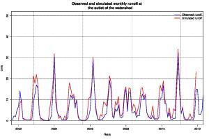
2002. 2004. 2006. 2008. 2010. 2012. 0. 10. 20. 30. 40. 50. Years cm/s. Observed and simulated monthly runoff at the outlet of the watershed. Observed runoff.

R Graphics Output -
Page 1. 100. 150. 200. 250. 300. 350. −15. −10. −5. 0. 5. 10 inla.group(agb, n = 100). PostMean 0.025% 0.5% 0.975%

R Graphics Output -
Page 1. q q q q q q q q q q q q. −9. −7. −5. −3. −1. 1. 3. 5. 01/17. 04/17. 07/17. 10/17. 01/18. Short−term changes (%) q q. Gross. Corrected.

R Graphics Output -
Page 1. q. 0.50. 0.75. 1.00. 1.25. 1.50. 0.50. 0.75. 1.00. 1.25. 1.50. 1. 1 test.

R Graphics Output -
0. 1. 2. 3. 4. 0. 100. 200. 300. 400. N55F 2017−05−04. Small−Scale. Time−lag (minutes). Semi−variance (square meters) q q q q q q. q q q q. q q q. q q q.

R Graphics Output -
2008 2009 2010 2011 2012 2013 2014 2015 2016. Clear Channel. PBSC/BIXI. BCycle. SandVault. Arcade. SOBI. Nextbike. Bewegen. Year. Number of systems ...

R Graphics Output -
Page 1. long lat. 60. 62. 64. 66. 68. 70. −60. −50. −40. −30. −20.