PHYSICAL REVIEW B 78, 144302 共2008兲
Quasiharmonic elastic constants corrected for deviatoric thermal stresses Pierre Carrier,1 João F. Justo,2 and Renata M. Wentzcovitch1 1Minnesota
Supercomputing Institute, Department of Chemical Engineering and Materials Science, University of Minnesota, Minneapolis, Minnesota 55455, USA 2Escola Politécnica, Universidade de São Paulo, CP 61548, CEP 05424-970 São Paulo, SP, Brazil and Chemical Engineering and Materials Science Department, University of Minnesota, Minneapolis, Minnesota 55455, USA 共Received 6 August 2008; revised manuscript received 23 September 2008; published 21 October 2008兲 The quasiharmonic approximation 共QHA兲, in its simplest form also called the statically constrained 共SC兲 QHA, has been shown to be a straightforward method to compute thermoelastic properties of crystals. Recently we showed that for noncubic solids SC-QHA calculations develop deviatoric thermal stresses at high temperatures. Relaxation of these stresses leads to a series of corrections to the free energy that may be taken to any desired order, up to self-consistency. Here we show how to correct the elastic constants obtained using the SC-QHA. We exemplify the procedure by correcting to first order the elastic constants of MgSiO3 perovskite and MgSiO3 postperovskite, the major phases of the Earth’s lower mantle. We show that this first-order correction is quite satisfactory for obtaining the aggregated elastic averages of these minerals and their velocities in the lower mantle. This type of correction is also shown to be applicable to experimental measurements of elastic constants in situations where deviatoric stresses can develop, such as in diamond-anvil cells. DOI: 10.1103/PhysRevB.78.144302
PACS number共s兲: 65.40.⫺b, 91.35.⫺x, 91.60.Gf
I. INTRODUCTION
The quasiharmonic approximation 共QHA兲 共Refs. 1 and 2兲 is a computationally efficient method for evaluating thermal properties of materials within the density-functional theory 共DFT兲 from low to temperatures above the Debye temperature. It provides high quality high-pressure–high-temperature materials properties3–8 in a continuous pressure-temperature 共PT兲 domain in which anharmonic effects are negligible.9 However, it has a not well recognized shortcoming: the nonhydrostatic nature of thermal stresses in nonisotropic structures. Broadly speaking, these calculations start by obtaining the static internal energy of fully relaxed DFT structures at various pressures. After computations of the vibrational density of states, the thermal energy contribution to the Helmholtz free energy is added. This latter contribution has anisotropic strain gradients and produces deviatoric stresses. This straightforward procedure should be referred to as the statically constrained 共SC兲 QHA. It has been used to compute the elastic constant tensor of isotropic3 and nonisotropic minerals4,6 at high PT as well, even though pressure conditions were not precisely hydrostatic in the latter calculations. In general, relaxation of deviatoric stresses, irrespective of their origin, is essential in both experiments10 and theory9 for generating realistic and reproducible structural and elastic properties. Here we show how to correct the elastic constant tensor obtained using the SC-QHA. We exemplify the procedure by correcting to first order the elastic constants of MgSiO3 perovskite 共PV兲 and MgSiO3 postperovskite 共PPV兲, the major phases of the Earth’s lower mantle, for which elasticity data are essential to interpret seismic information of this region.11 We show that this first-order correction is quite satisfactory for obtaining the aggregated elastic averages of these minerals and their acoustic velocities in the PT range of the lower mantle. This article is organized as follows: we first discuss the equations used for numerically determining the elastic con1098-0121/2008/78共14兲/144302共6兲
stant tensor within the SC-QHA. We then describe the procedure for correcting it to first order for deviatoric thermal stresses. We then evaluate these corrections to the previously reported elastic constant tensors of PV 共Ref. 4兲 and PPV.6 II. ELASTICITY WITHIN AND BEYOND THE STATICALLY CONSTRAINED QHA
The present procedure builds on a related procedure to correct structural parameters and equations of state of nonisotropic solids at high PTs.9 The method introduced in Ref. 9 can correct the SC crystal structure at V共P , T兲 to infinite order as long as the SC elastic constant tensor is simultaneously corrected. However, this is a very demanding computational procedure and, fortunately, unnecessary. A firstorder correction to the crystal structure using the SC elastic constant appears to be sufficient. This conclusion was reached after examining the crystal structure of one of the most studied materials at high PT: MgSiO3 perovskite.12 This type of experimental data is quite limited and results on other materials with similarly complex crystal structures would be helpful to strengthen this conclusion. According to the 共SC兲 QHA the Helmholtz free energy is given by
冋
F共V,T兲 = E共V兲 + 兺 qj
册
បqj共V兲 + kBT 兺 ln共1 − e−បqj共V兲/kBT兲, 2 qj 共1兲
where kB and ប are, respectively, Boltzmann’s and Planck’s constants. The first term, E共V兲, is the volume-dependent static energy obtained after full structural relaxation under isotropic pressure, and 共V兲 is the corresponding phonon spectrum. Both phonon spectrum and static energy are here determined using the DFT within the local-density approximation 共LDA兲,13 but the methodology is general and applicable to any first-principles method. Structural relaxations
144302-1
©2008 The American Physical Society
PHYSICAL REVIEW B 78, 144302 共2008兲
CARRIER, JUSTO, AND WENTZCOVITCH
are performed using a variable cell shape 共VCS兲 algorithm,14 and phonon spectra are computed using the PWSCF code15 as described in Ref. 16, based on the linear-response theory. The second term in Eq. 共1兲 is the zero-point energy, FZP, such that the sum of the terms in the brackets is the energy at T = 0 K. The last term in Eq. 共1兲 is the thermal excitation energy, Fth 共see Ref. 2 for details兲. Pressure, P, is obtained from F using the standard thermodynamics relation
冏 冏
P=−
F V
共2兲
. T
This procedure implicitly assumes that P remains isotropic at all temperatures, but this is only true for static calculations, where structures were optimized at target pressures. The two frequency dependent terms in Eq. 共1兲, the zero-point energy and the thermal energy, contribute to P but their strain gradients are intrinsically anisotropic. This effect was recently quantified9 by the computation of deviatoric thermal stresses, ␦k, defined as the difference between the stress tensor and the nominal pressure 共diagonal兲 tensor. In Voigt’s notation
␦k =
冏
1 G共P,T兲 V0 ⑀k
冏
− H共3 − k兲P,
for
k = 1, . . . ,6,
P,T
共3兲 where H共n兲 is the Heaviside step function, equal to 0 for 共3 − k兲 strictly negative and 1 otherwise. Deviatoric thermal stresses are caused by the vibrational 共zero-point and thermal兲 energies and are shown to be important at high pressures and temperatures. The larger the temperature, the more visible these stresses are. We have previously shown that these deviatoric stresses can be relaxed to first order if one knows the elastic constant tensor, cij共P , T兲, calculated within the 共SC兲 QHA.9 The latter are obtained from the Gibbs free energy, G,
h쐓 = h共I − ⑀兲, where
冢
ax bx cx h = ay by cy az bz cz
冏
冏
.
6
+
兺 m=1
冣
2cij ⑀k ⑀l
⑀k P,T
⑀ k⑀ l + . . . .
共8兲
P,T
Neglecting second and higher order terms one has cij共P,T, ⑀兲 = ⯝ cij共P,T兲 6
+兺
6
兺 k=1 m=1
冏 冏冏 冏冏 冏
=cij共P,T兲 +
cij P
P,T
P m
P,T
m ⑀k
冏 冏 兺冏 冏 cij P
3
P,T m=1
P m
⑀k , P,T
␦m .
共9兲
P,T
In the last step above we assumed that pressure is unaffected by shear stresses, i.e., 兩 P / m 兩 P,T = 0 for m = 4, 5, and 6, thus reducing the index summation from 6 to 3. The stress derivatives of P in Eq. 共9兲 are determined using the definition of the pressure as the trace of the stress tensor, P 3 m. Taking the derivative of the pressure as func⬅ 1 / 3 兺m=1 tion of each stress leads to 兩 P / m 兩 P,T = 1 / 3 , for m = 1, 2, and 3. Therefore the first-order corrected elastic constants at the strains given by Eq. 共6兲 is reduced to cij共P,T, ⑀1, ⑀2, ⑀3兲 = cij共P,T兲 +
共6兲
The Cartesian components of the relaxed lattice vectors are then
6
k=1 l=1
6
⑀k共P,T兲 =
cij ⑀k
k=1
T
−1 ckm 共P,T兲␦m .
冏 冏 冏 兺 兺冏
cij共P,T, ⑀兲 = cij共P,T,0兲 + 兺
共5兲
The adiabatic elastic constants, which are the relevant ones for interpretation of seismic data, are then computed using appropriate thermodynamics relations.4,18 Below all calculated elastic constants, bulk and shear moduli, and velocities are adiabatic. Lattice parameters at high pressures and temperatures under hydrostatic conditions can then be corrected to first order by evaluating the strains, ⑀k, involved in the relaxation of the deviatoric thermal stresses given in Eq. 共3兲
冢
6
by calculating the second derivative of G with respect to the strains ⑀i and ⑀ j:4,17 1 2G cij共P,T兲 = V0 ⑀i ⑀ j
冣
⑀1 ⑀6/2 ⑀5/2 ⑀ = ⑀6/2 ⑀2 ⑀4/2 ⑀5/2 ⑀4/2 ⑀3
and
are, respectively, the matrices of lattice vectors 共aជ , bជ , cជ 兲 and Cartesian strains 共keeping up with Voigt’s notation兲. Notice that increase in symmetry or symmetry break 共phase transformations兲 may be induced by deviatoric thermal stresses in the presence of soft phonon, i.e., h and h쐓 do not necessarily have to the same space group. In Ref. 9 we pointed that attainment of zero deviatoric thermal stresses within the QHA should involve a selfconsistent cycle with simultaneous recalculation of the elastic constant tensor under hydrostatic condition followed by new structural relaxation, and so on. However, such procedure is extremely computationally intensive given the need to recompute vibrational density of states on a PT grid every step of the cycle. We show next how to obtain the elastic constant tensor corrected to first order with knowledge of Eq. 共6兲 only. The components of the elastic constant tensor expanded in a Taylor series of strains 共in Voigt’s notation兲 defined by Eq. 共6兲 are
共4兲
G共P,T兲 = F + PV
共7兲
冏 冏
1 cij 3 P
␦⌺ ,
共10兲
P,T
3 ␦k. This correction requires only knowlwhere ␦⌺ = 兺k=1 edge of the pressure derivatives of cij’s which are known from the statically constrained QHA calculation, and the de-
144302-2
PHYSICAL REVIEW B 78, 144302 共2008兲
QUASIHARMONIC ELASTIC CONSTANTS CORRECTED FOR…
101
δσ1 (GPa)
1−ε 1 (%) 4000 K
(a)
4000 K
3000 K
4000 K
1000 K 0K
99.5
0K 1000 K
100.5 100
99.5 2000 K 99
1−ε 3 (%)
2 1 0 K 1000 K 0 -1 2000 K 3000 K -2 100 50
100
3000 K
99
4000 K
δσ 3 (GPa)
2 3000 K 2000 K 1 0 -1 1000 K 0K -2
100.5 2000 K
1−ε 2 (%)
δσ2 (GPa)
2 1 0 K 1000 K 0 -1 2000 K 3000 K -2
4000 K 150
P (GPa)
200
100.5 2000 K 3000 K 4000 K 100 K 99.5 1000 0K 99 100 50 150 P (GPa) (b)
200
FIG. 1. 共Color online兲 共a兲 Deviatoric thermal stresses in PPV; 共b兲 percentage lattice-constant corrections in PPV. ␦1 and ␦2 have opposite signs and similar magnitude, similarly to the case of PV 共Ref. 9兲. However, ␦3 in PPV is considerably larger than in PV.
their corresponding stresses are therefore also available from experiments. Pressure variation in the elastic constants22 are measurable quantities23 that require only few additional runs for estimating experimentally the pressure derivative of cij at given PT’s. Eventual experimental setting that combines simultaneously measurements of 共i兲 and 共ii兲 above can be used to measure the correction to the elastic constants due to deviatoric stresses in DAC apparatus after applying Eq. 共10兲. III. ELASTIC CONSTANTS OF PV AND PPV
We present in this section new results on the deviatoric thermal stresses of PPV and the correction to the elastic con-
δσ Σ (GPa)
1 0.8 0.6 0.4 0.2 0 -0.2 -0.4 (a) 0 0 -0.2 -0.4 -0.6 -0.8 -1 -1.2 -1.4 -1.6 50
δσ Σ (GPa)
viatoric thermal stresses given by Eq. 共3兲. It gives to first order the elastic constants corrected for deviatoric stresses without having to explicitly calculate Gibbs free energy at the relaxed lattice parameters. The correction is a general approach to elasticity to be applied within the limit of validity of the quasiharmonic approximation. We have not addressed elasticity beyond this limit, which should somehow include anharmonic corrections. Here it is assumed that the free energy 关Eq. 共1兲兴 is computed correctly at high temperatures and that all appropriate excitations are accounted for, including in general electronic thermal and magnetic ones. Electronic thermal excitations are important in metals.8 The standard method for dealing with metals is to perform DFT calculations using the Mermin functional.19,20 Phonon frequencies also can be much affected by these excitations and the calculated thermodynamics properties.21 In magnetic systems the magnetic 共spin兲 excitations also need to be included in the computation of free energies of Eq. 共1兲. These can be in the form of magnons 共for metals or insulators兲, or in the form of a pure entropy term in the case of paramagnetic insulators.21 As far as the free energy of the system in consideration is properly computed, the current scheme provides a method for obtaining elastic constants to arbitrary accuracy by iterating the computations of elastic constants to arbitrary order. As a final remark, we point that Eq. 共10兲 could also be used and tested on experimental data as a mean for correcting any type of deviatoric stresses, as long as the stress deviations remain small compared to the hydrostatic pressure 共in a limit for the Taylor expansion to be valid兲. The correction only requires knowledge of 共i兲 the three components ␦k, k = 1 , 2 , 3, and at the same time 共ii兲 the pressure variac tion in the elastic constants at specified P and T: 兩 Pij 兩 P,T. Principal strain deviations, ⑀⬜ and ⑀储, are measurable quantities, for instance, using diffraction ring measurements10 and
(b)
2000
1000 K
30
00
K
K
4000
K
0K
100
50
150
0K
1000 K 2000 K
100
3000
K
P (GPa)
4000 K
150
200
FIG. 2. 共Color online兲 Sum of diagonal deviatoric stresses for 共a兲 PV and 共b兲 PPV, as defined in Eq. 共10兲. This sum is considerably larger in PPV because of the larger contribution from ␦3 in PPV. Note that the pressure ranges between PV and PPV differ, corresponding to their respective QHA regions of validity 共Ref. 9兲.
144302-3
PHYSICAL REVIEW B 78, 144302 共2008兲
CARRIER, JUSTO, AND WENTZCOVITCH 1
8 7
dC33 /dP
dC22 /dP
dC11 /dP
4
dC12 /dP dC /dP 13
dC13 /dP
(a)
0
dC66 /dP
dC55 /dP
1 0
50
100
P (GPa)
150 0
100
50
P (GPa)
150 0
50
100
P (GPa)
150
(a)
δ K [GPa]
0K 3000 K
dC33 /dP
dC11 /dP
0 50
3000 K
dC23 /dP
dC13 /dP dC66 /dP
Shear moduli correction
50
P [GPa]
150
P (GPa)
200 50
100
150
P (GPa)
100
150
0K
-1
1000 K K 2000
4000 K
3000 K
200 50
100
0K
-1
1000 K 2000 K
150
P (GPa)
200
FIG. 3. 共Color online兲 Derivatives of elastic constants as function of pressure of 共a兲 PV and 共b兲 PPV. See also note in the caption of Fig. 2.
stants obtained using the 共SC兲 QHA.6 Since deviatoric thermal stresses of PV were recently published,9 we also give here the corresponding correction to the elastic constants of PV. The PT dependent elastic constant tensors of PV and PPV determined using the 共SC兲 QHA have been reported, respectively, in Refs. 4 and 6. These are the major phases of the Earth’s lower mantle and their elastic properties are central information for the interpretation of the seismic properties of this inaccessible region in terms of temperature, composition, and mineralogy. PV and PPV are both orthorhombic crystals, respectively, with symmetry Pbnm and Cmcm. This difference of symmetry group implies in particular, as stated in Ref. 6, that “the 关100兴PPV, 关010兴PPV, and 关001兴PPV direc¯ 0兴 , tions in the Cmcm structure correspond to the 关11 PV 关110兴PV, and 关001兴PV in the Pbnm structure, respectively,” corresponding to a rotation of 45° of the aជ -bជ reciprocal lattices. Lattice deformations and deviatoric thermal stresses between PV and PPV are thus comparable only through this transformation. Figure 1共a兲 shows the deviatoric thermal stresses for PPV. Equivalent results for PV have recently been reported in Ref. 9 along with the analysis of its crystalline structure at high PT. The deviatoric stresses ␦1 and ␦2 in PPV have opposite sign but similar magnitudes to that of
(b)
-3 50
4000 K
3000 K
-2
dC44 /dP
dC55 /dP
100
4000 K
0K
-1 0
-3 0 δ G [GPa]
dC ij/dP (b)
2000 K
Bulk moduli correction
dC12 /dP
2 1
1000 K
0
dC22 /dP
4 3
4000 K
Bulk moduli correction
0.5
-2
5
0K
0K
0
7
300
-0.5
dC44 /dP
8
6
1000 K
0
K
-1 1
3 2
2000
0.5
-0.5
5
δ G [GPa]
dC ij /dP
6
δ K [GPa]
0K 3000 K
Shear moduli correction
100
P [GPa]
150
200
FIG. 4. 共Color online兲 Corrections to the bulk and shear moduli for 共a兲 PV4 and 共b兲 PPV.7
PV 共see Ref. 9兲, except along the cជ crystalline axes. As stated above, deviatoric thermal stresses for PV and PPV induce distinct deformations along lattices aជ and bជ . The deviatoric thermal stresses in the z direction of PPV is considerably larger than the corresponding one in PV leading to larger corrections in PPV than in PV, as shown below. Figure 1共b兲 shows the percentage corrections to the lattice parameters of PPV, based on Eq. 共6兲. Interestingly, Fig. 1 shows that zeropoint energy 共the black zero Kelvin line in that figure兲 also produces deviatoric stresses. With increasing temperature, these stresses are enhanced but their origin is the anisotropic nature of the phonon dispersions. Figure 2 shows the resulting summation of the three deviatoric thermal stresses ␦⌺ 关of Fig. 1共a兲兴 for PPV 共and see Ref. 9 for PV’s deviatoric thermal stresses兲. It represents the first of the two ingredients necessary for the correction given by Eq. 共10兲. Clearly, the correction for PPV is considerably larger than the one for PV. This is mostly due to ␦3 that is larger in PPV than in PV 共see above兲. The correction for PPV is always negative, which has the effect of decreasing its elastic constants, while for PV, the correction can be negative 共mostly at low temperature兲 or positive 共mostly at high temperature兲. In principle, there are no reasons for having deviations of systematic nature and they should vary depending on the crystalline structure. One observation that remains true
144302-4
PHYSICAL REVIEW B 78, 144302 共2008兲
QUASIHARMONIC ELASTIC CONSTANTS CORRECTED FOR…
for all crystalline structures, however, is that positive deviations in one direction are to be compensated by a negative deviation in another direction, as observed in both PV and PPV. Figure 3 shows the pressure derivatives, cij / P, of all the elastic constants of PV and PPV, which is the second ingredient required for the correction according to Eq. 共10兲. The figure shows the variations in cij with pressure for only two temperatures, 0 and 3000 K, the latter being close to the temperature of the D⬙ layer in the lower mantle, where the PPV phase is important in the geophysical models.11 Figure 4 shows the corrected bulk and shear moduli, after applying Hill’s24 共arithmetic兲 average to the elastic constants, at several temperatures. The corrections are largest at high pressure and high temperature in both PV and PPV. The nature of the correction is also structure dependent. Notice that the general aspect of the correction to the bulk moduli in Fig. 4 is similar to ␦⌺ displayed in Fig. 2, indicating that the dominant term in the correction of Eq. 共10兲 is the deviatoric thermal stress, and to a lesser extent the pressure derivatives of the elastic constants. However, all corrections remain relatively small, meaning the 共SC兲 QHA calculation does not suffer from significant deviatoric thermal stresses, although they can very well be corrected to any level of accuracy. Table I summarizes the corrections to the 共SC兲 QHA for the elastic constants at T = 3000 K for two pressures, P = 100 GPa and P = 120 GPa. Corrections are given in parentheses. Bulk and shear moduli calculated using Voigt 共uniform strain兲, Reuss 共uniform stress兲, and Hill 共arithmetic average between Voigt and Reuss兲 are shown.24 The volume correction, abc ⫻ 共1 − ⑀1兲共1 − ⑀2兲共1 − ⑀3兲, as shown in Fig. 1共b兲, is reported as density 共P , T兲. Velocities are then evaluated from Voigt-Reuss-Hill moduli since it provides a realistic estimation of the true moduli. Notice that velocities are only slightly modified because moduli are corrected along with the density; therefore, their ratio remains relatively unaltered.
TABLE I. Elastic moduli of PV 共Ref. 4兲 and PPV 共Ref. 7兲 with corrections given in parenthesis as described by Eq. 共10兲. Pressure and elastic constants are in GPa, velocities in km/s, temperature in K, densities, , in g / cm3. The corrections are significant for bulk and shear moduli. Velocities are only slightly changed by the correction. V P = 冑共KH + 4 / 3GH兲 / , VS = 冑GH / , V⌽ = 冑KH / , and ⌽ = KH / , where upper indices R, V, and H represent Reuss, Voigt, and the Hill averages 共Ref. 24兲. Notice that ⌽ = V2P − 4 / 3V2S. Velocities are calculated using the Hill averages. Decimal digits are presented to show the magnitude of the corrections. However, except for , the accuracy of results should not include decimal digits.
IV. CONCLUSIONS
for computing high PT elastic constants to the desired level of accuracy.
In summary, we have introduced a scheme to correct high PT elastic constants obtained using the statically constrained quasiharmonic approximation for deviatoric thermal stresses that develop in calculations of anisotropic structures. This self-consistent scheme was used to compute to first order the elastic constants of the geophysically important MgSiO3 perovskite and MgSiO3 postperovskite phases of the lower mantle. The corrections introduced by relaxation of these deviatoric stresses are quite small at relevant conditions of the lower mantle and previous 共SC兲 QHA results remain essentially unchanged. However, this might not be the general case and the current scheme may be used to arbitrary order
3000 K, 100 GPa PV PPV c11 c22 c33 c44 c55 c66 c12 c13 c23 KV KH KR GV GH GR VP VS V⌽ ⌽
774.8共0.0兲 941.7共0.0兲 928.5共0.0兲 287.2共0.0 251.0共0.0兲 248.4共0.0兲 452.7共0.0兲 373.9共0.0兲 406.5共0.0兲 567.9共0.0兲 565.2共0.0兲 562.4共0.0兲 251.4共0.0兲 249.2共0.0兲 247.0共0.0兲 5.04共0.00兲 13.35共0.00兲 7.03共0.00兲 10.59共0.00兲 112.20共0.02兲
3000 K, 120 GPa PV PPV
933.4共−3.3兲 844.4 共0.3兲 1069.5共−2.8兲 756.0共−2.1兲 1049.9 共0.5兲 846.8共−1.9兲 949.0共−2.9兲 1034.9 共0.5兲 1072.5共−2.6兲 215.8共−1.7兲 313.6 共0.1兲 286.6共−1.4兲 164.4共−1.1兲 265.6 共0.1兲 211.1共−1.0兲 253.3共−1.6兲 276.4 共0.1兲 314.9共−1.2兲 376.7共−1.3兲 520.4 共0.3兲 433.4共−1.2兲 370.6共−1.0兲 421.3 共0.2兲 413.3共−0.9兲 434.3共−1.1兲 455.7 共0.2兲 481.1共−1.0兲 555.7共−1.7兲 636.0 共0.3兲 627.2共−1.5兲 553.3共−1.7兲 632.2 共0.3兲 624.3共−1.5兲 550.8共−1.7兲 628.4 共0.3兲 621.5共−1.5兲 223.8共−1.2兲 273.3 共0.1兲 273.3共−1.0兲 219.5共−1.2兲 270.1 共0.1兲 268.6共−1.0兲 215.2共−1.2兲 267.0 共0.1兲 263.9共−1.0兲 5.11共−0.01兲 5.22 共0.00兲 5.29共−0.01兲 12.87共−0.01兲 13.79 共0.01兲 13.63共−0.01兲 6.56共−0.01兲 7.20 共0.00兲 7.13共−0.01兲 10.41共−0.01兲 11.01 共0.00兲 10.86共0.00兲 108.33共−0.10兲 121.21 共0.06兲 118.02共−0.11兲
ACKNOWLEDGMENTS
This work was supported by NSF Grants No. EAR0230319, No. EAR-0635990, and No. ITR-0428774. We especially thank Shuxia Zhang from the Minnesota Supercomputing Institute for her assistance with optimizing the PWscf code performance on the BladeCenter Linux Cluster and on the SGI Altix XE 1300 Linux Cluster, and Yonggang Yu for helpful discussions relative to PWscf. PC acknowledges partial support from a MSI research scholarship and JFJ from Brazilian agency CNPq.
144302-5
PHYSICAL REVIEW B 78, 144302 共2008兲
CARRIER, JUSTO, AND WENTZCOVITCH D. C. Wallace, Thermodynamics of Crystals 共Dover, Mineola, 1972兲. 2 O. L. Anderson, Equations of State of Solids for Geophysics and Ceramic Science 共Oxford University Press, New York, 1995兲. 3 B. B. Karki, R. M. Wentzcovitch, S. de Gironcoli, and S. Baroni, Science 286, 1705 共1999兲. 4 R. M. Wentzcovitch, B. B. Karki, M. Cococcioni, and S. de Gironcoli, Phys. Rev. Lett. 92, 018501 共2004兲. 5 X. Sha and R. E. Cohen, Phys. Rev. B 74, 064103 共2006兲. 6 T. Tsuchiya, J. Tsuchiya, K. Umemoto, and R. M. Wentzcovitch, Earth Planet. Sci. Lett. 224, 241 共2004兲; R. M. Wentzcovitch, T. Tsuchiya, and J. Tsuchiya, Proc. Natl. Acad. Sci. U.S.A. 103, 543 共2006兲. 7 R. M. Wentzcovitch, T. Tshuchiya, and J. Tsuchiya, Proc. Natl. Acad. Sci. U.S.A. 103, 543 共2006兲. 8 E. Menéndez-Proupin and A. K. Singh, Phys. Rev. B 76, 054117 共2007兲. 9 P. Carrier, R. Wentzcovitch, and J. Tsuchiya, Phys. Rev. B 76, 064116 共2007兲; 76, 189901 共2007兲. 10 W. A. Bassett, J. Phys.: Condens. Matter 18, S921 共2006兲. 11 K. Hirose, J. Brodholt, T. Lay, and D. Yuen, Post-Perovskite: The Last Mantle Phase Transition, Geophysical Monograph Series Vol. 174 共American Geophysical Union, Washington DC, 2007兲, p. 350. 12 G. Fiquet, D. Andrault, A. Dewaele, T. Charpin, M. Kunz, and D. Hausermann, Phys. Earth Planet. Inter. 105, 21 共1998兲; N. Funamori, T. Yagi, W. Utsumi, T. Kondo, T. Ushida, and M. Funamori, J. Geophys. Res. 101, 8257 共1996兲; N. Ross and R. 1
Hazen, Phys. Chem. Miner. 16, 415 共1989兲; 17, 228 共1990兲; W. Utsumi, N. Funamori, T. Yagi, E. Ito, T. Kikegawa, and O. Shimomura, Geophys. Res. Lett. 22, 1005 共1995兲; Y. Wang, D. Weidner, R. Liebermann, and Y. Zhao, Phys. Earth Planet. Inter. 83, 13 共1994兲. 13 P. Hohenberg and W. Kohn, Phys. Rev. 136, B864 共1964兲; W. Kohn and L. J. Sham, ibid. 140, A1133 共1965兲. 14 R. M. Wentzcovitch, Phys. Rev. B 44, 2358 共1991兲. 15 S. Baroni, A. Dal Corso, S. de Gironcoli, P. Giannozzi, C. Cavazzoni, G. Ballabio, S. Scandolo, G. Chiarotti, P. Focher, A. Pasquarello, K. Laasonen, A. Trave, R. Car, N. Marzari, and A. Kokalj 共http://www.pwscf.org/兲. 16 S. Baroni, S. de Gironcoli, A. Dal Corso, and P. Giannozzi, Rev. Mod. Phys. 73, 515 共2001兲. 17 J. F. Nye, Physical Properties of Crystals, Their Representation by Tensors and Matrices 共Clarendon, Oxford, 1985兲. 18 M. J. P. Musgrave, Crystal Acoustics, Introduction to the Study of Elastic Waves and Vibrations in Crystals 共Holden-Day, San Francisco, 1970兲. 19 D. Mermin, Phys. Rev. 137, A1441 共1965兲. 20 R. M. Wentzcovitch, J. L. Martins, and P. B. Allen, Phys. Rev. B 45, 11372 共1992兲. 21 T. Tsuchiya, R. M. Wentzcovitch, C. R. S. da Silva, and S. de Gironcoli, Phys. Rev. Lett. 96, 198501 共2006兲. 22 W. B. Daniels and C. S. Smith, Phys. Rev. 111, 713 共1958兲. 23 A. K. Singh, H.-k. Mao, J. Shu, and R. J. Hemley, Phys. Rev. Lett. 80, 2157 共1998兲. 24 R. Hill, Proc. Phys. Soc., London, Sect. A 65, 349 共1952兲.
144302-6