Pseudo-spectral modeling in geodynamo Maxim Reshetnyak and Bernhard Steffen John von Neumann Institute for Computing (NIC), Central Institute for Applied Mathematics (ZAM), Research Centre J¨ulich, 52425 J¨ulich, Germany Many stars and planets have magnetic fields. The heat flux causes 3D convection of plasma or metal, which can generate a large-scale magnetic field like that observed. The small-scale behavior, demonstrating self-similarity in a wide range of the spatial and temporal scales, is a field of active research using modeling, as it is usually not observed. Rapid rotation gives a geostrophic system, where convection degenerates in the direction of the axis of rotation and all variation along this axis is weak. Such a system is somewhere in between the full 3D and 2D-systems. Its special properties show up in the physical and the spectral space simultaneously. Pseudo-spectral modeling solves the PDE in spectral space for easy calculations of integrals and derivatives. The nonlinear terms are calculated physical space, requiring many direct and inverse FFTs per time step. We apply this technique to the thermal convection problem with heating from below in a Cartesian box. Above a threshold of the kinetic energy the system generates the magnetic field. The most time consuming part of our MPI code is FFT transforms. For efficiency, we selected a FFT library which makes use of the symmetry of the fields. The optimal number of processors is ∼ half the number of grid planes, with superlinear speedup. The single node performance is poor, each processor delivering only ∼ 5% of its peak rate. We see cyclonic convection with a cyclone density of the ∼ E −1/3 (E Ekman number ∼ 10−15 for earth). This causes a high anisotropy of the convection even for high Reynolds numbers. Our simulations demonstrates the generation of the large-scale hydrodynamic helicity. Helicity is an integral of the Navier-Stokes equation, and it has close relation to the α-effect which generates the large scale magnetic field via the small-scale turbulence. This process has three stages:. At first, the magnetic field grows exponentially from a small seed. When the magnetic and kinetic energies are comparable the growth slows down, and finally equilibrium is reached. The magnetic field again quenches the helicity, damping primarily the toroidal part of velocity field. It slows down the rotation of the cyclones (anti-cyclones). The helicity causes a divergence (convergence) of the cyclones near the upper (lower) boundaries (z = 0, 1). It is generated at the boundaries and transported to center of the box. It changes sign at the middle of the box. Convection and dynamo systems are dissipative, so the equilibrium of the system in sense of the statistical mechanics is not reached. The kinetic energy is injected into the system at the medium scale of cyclons, one sink of energy is at the small viscous scale, another at the large (magnetic field) scale. For some (small) scales the cascade of the energy is direct (like it is in the Kolmogorov’s like turbulence), for others (larger than cyclones) it is inverse, like it is observed in 2D turbulence. At the small scales there is a constant energy flux, as is plausible as from theorie and from semi-empirical models.
1 Introduction Almost all stars, the earth, and the planets larger than earth have large scale magnetic fields that are believed to be generated by a common universal mechanism - the conversion of kinetic energy into magnetic energy in a turbulent rotating shell. The details, however, - and thus the nature of the resulting field - differ greatly. The only fields observable with good accuracy are that of the earth and of the sun. The challenge for the dynamo theory is to provide a model that can explain the visible features of the field with realistic
1
assumptions on the model parameters. Calculations for the entire star or planets are done either with spectral models6 or finite volume methods12 , and have demonstrated beyond reasonable doubt that the turbulent 3D convection of the conductive fluid -in the core for earth, in an upper shell for the sun - can generate a large scale magnetic field similar to the one observed out of small random fluctuations. However, both these methods cannot cover the enormous span of scales required for a realistic parameter set. For the geodynamo, the time scale of the large scale convection is ∼ 103 years, during which the planet itself makes ∼ 106 revolutions. Further on, viscosity operates at a scale of centimeters, compared to the convective scale of ∼ 106 meters. Thus the effects of the small scale processes have to be averaged and transported to the finest scale resolved, which will be orders of magnitude larger. For the sun and other stars, the situation is not better, the difference of scales being frequently even larger. To verify the averaging approaches and to understand the interactions of the different scales of turbulence, calculations of small parts of the earth’ core are required, at least partially bridging the gap in scale. For this, we look at a the thermal convection problem (in Boussinesque approximation) with heating below in a Cartesian box at the equatorial plane.
2 The equations The geodynamo equations for the incompressible fluid (∇ · V = 0) in the volume of the scale L rotating with the angular velocity Ω in the Cartesian system of coordinates (x, y, z) in its traditional dimensionless form in physical space can be written as follows: ∂B = ∇ × (V × B) + q−1 ∆B ∂t � � −1 ∂V Pr + (V · ∇) V = −∇P − 1z × V + Ra T z1z + (∇ × B) × B + E ∆V E ∂t ∂T + (V · ∇) (T + T0 ) = ∆T + G(r). ∂t (1) −1 2 The velocity V, magnetic field B, pressure P = p + Pr V /2 and typical diffusion E p time t are measured in units of κ/L, 2Ωκµρ;, ρκ2 /L2 and L2 /κ respectively, where κ is the Prandtl number, κ is thermal diffusivity, ρ is density, µ permeability, Pr = ν ν is the Ekman number, ν is kinematic viscosity, η is the magnetic diffusivity, E= 2ΩL2 αg0 δT L is the modified Rayleigh number, and q = κ/η is the Roberts number. Ra = 2Ωκ α is the coefficient of volume expansion, δT is the unit of temperature (see for more details5 ), g0 is the gravitational acceleration, and G is the heat source. For boundary conditions, we assume a temperature gradient from the lower to the upper boundary large enough to drive a convection, and periodicity otherwise, which leads to odd or even symmetry relative to the equator. Some features of the field can be seen from a dimensional analysis already. The extreme smallness of the Ekman number means that the terms without E must almost cancel out, which without magnetic field results in a geostrophic balance where all fluxes transverse to the rotation are blocked by the Coriolis force and cyclonic motion is generated. With the magnetic field, a magnetostrophic balance or a mixture seems possible, depending on
2
the scale considered. The direct numerical integration of these equations is not efficient, much larger time steps and easier calculations can be achieved by transforming the equations into wave space. Also, some features of the solution show up much better in wave space than in physical space, and especially the separation of scales becomes clear there. Because the calculations of the nonlinear terms in wave space would be full matrix operations, they have to be done in physical space, requiring FFT transform of all quantities in every time step, which will dominate the computing time. After elimination of the pressure using k · V = 0, k · B = 0 and transforming the equations into wave space we come to1 � � ∂B + q−1 k 2 B = [∇ × (V × B)]k k � �∂t −1 ∂V 2 + k V = kPk + Fk (2) E Pr ∂t� k � ∂T + k 2 T = − [(V · ∇) T ]k + G(k) ∂t k with
Pk = −
k · Fk , k2
k 2 = kβ kβ ,
β = 1...3 (3)
� � Fk = Pr−1 V × (∇ × V) + Ra T 1z − 1z × V + (B · ∇) B k .
For integration in time we use explicit Adams-Bashforth (AB2) scheme for the non-linear terms. The linear terms are treated using the Crank-Nicolson (CN) scheme. To resolve the diffusion terms we used a well known trick which helps to increase the time step significantly. We rewrite scheme.
∂A ∂t
+ k 2 A = U in the form
0 γt
∂Aek ∂t
= U ek
2
γt
and then apply the CN
3 Parallel FFT for the equations The program shows slightly superlinear speedup up to processor number of half the number of physical planes, so parallelizing is not a problem. However, the single node performance is a problem. The Fourier transforms dominate the computing times, in the implementation used they make up about 85%, so the FFTs are subject careful inspection. Special tests were done on a physical grid of 128*129*128 real values, (second dimension is logically 256 and even), and using 4 processors of jump for the calculations, both direct and inverse Fourier transform take slightly less than 6 ms each, with the difference less than the variations in the timings. The direct transforms is a transform from 3D real with symmetry in the second coordinate (due to the conventional placement of coordinates in geophysics), size nx*ny*nz, into a 3D complex array of slightly more than half the size, if redundancies are eliminated. There is no software available doing exactly this, not even sequentially. Therefore the FFT was put together from the sequential 1D FFT provided by9 based on11 ,13 , and some data movements in the following (natural) order: The data comes distributed on the processors
3
along the last component. As a first step, nx*nz transforms along the second component real even symmetric to real even symmetric or real odd symmetric to purely imaginary odd symmetric - are done using routine RDCT. (cosine transform) or RDST (Sine transform). After this, the array is transformed, such that now it is split along the second component. During the transform using mpi alltoallv, the second and third indices are exchanged for better access. Then nx*ny complex transforms in direction z follow, and finally ny*nz transforms in direction x. This procedure was chosen for ease of development and flexibility, it is reasonably fast but not optimal. An analysis using hardware counter monitoring (hpmcount,15) gave the following result:
load and store ops Instr. per cycle MFlips per sec user time Loads per TLB miss L2 cache miss rate
Cosine Trans
FFT compl
18.6 M 0.60 206 0.0516 3976 0.024
36.5 M 0.95 302 0.0782 257 0.116
reshape for alltoall 4.2 M 0.82 21.2 0.0098 21667 0.053
MPI alltoallv 0.065 M 1.310 0.0 0.006 22464 0.048
Both the cosine transform and the FFT include collecting the data to a stride 1 vector for every transform. According to gprof16 data, in a longer run the 3D FFT takes 34.5 s, of which only 14 s are spend in the 1D transforms, and 21.5 s in moving data (including the MPI call). It is now clear that the actual FFT is not more than half the time, assembling the data is of the same order, even though the processor efficiency of the FFT code is low, it runs at ∼ 5% of the peak performance. The main problem seems to be the TLB miss rate, though L2 and L3 cache misses are quite high, also. The inverse FFT performs the inverse operations in inverse order, the timing is almost the same. For optimization of the FFT, the first approach is using a better FFT routine. since the program development, a new release of FFTW3 has appeared which includes real symmetric FFT that was previously missing. It also contains provisions to do the ny plane FFTs in one step. Tests show FFTW to be faster than the FFT used till now. A second step is moving from complex-to-complex plane transforms to real-to-complex, as the result of the first transform is real or purely imaginary. This saves some data handling and half the communication volume. For the even symmetry the process is straightforward, for the odd symmetry, the final result has to be multiplied with the imaginary unit, which costs one sweep over the data. The third step is arranging the data in a way that memory access comes with as small a stride as possible. This means arranging the coordinates in an order different from the customary one, which is not an option during development of a program. It also requires changes in almost any part of the program, not only in the two subroutines organizing the FFT. All these together may cut the time for the FFT in half, which still means that it is the dominating part, so optimizing the implementation of other parts is not reasonable. While the tests were performed using a small number of processors, production runs use much more, such that each processor may contain only two or four planes of the grid for every quantity. This does effect our discussion above only with respect to the array
4
Figure 1. Thermal convection with rapid rotation (N = nx = ny = nz = 64) Pr = 1, Ra = 1.3 103 , E = 2 10−5 . for T (left column) (0, 1,0.43, 0.60), Vy (middle ) (−745, 548, −904, 979) and Vz (right) (−510, 501,−651, 784). The upper line corresponds to the section z = 0.5, and the lower to x = 0. The numbers are (min,max) values of the fields.
transform, which needs more but smaller messages for a larger number of processors. However, the communication time stays small up to 64 processors. Obviously, having more processors than planes in the grid would require a completely different organization.
4 Results 4.1 Pure convection, no magnetic field The thermal convection with a rapid rotation (Ro ≪ 1) is characterized by a large number of the vertical columns (cyclones and anticyclones). Their number depends on the Ekman number as kc ∼ E−1/32 . For the liquid core of the Earth E ∼ 10−15 , what is obviously prohibits simulations for the realistic range of parameters. Usually, one reach only with a E = 10−4 ÷ 10−65 . The second important parameter is a Rayleigh number describing intensity of the the heat sources. The critical Rayleigh number (when convection starts) depends on E as Racr ∼ E−1/3 . Further we consider three regimes: NR: Regime without rotation, Ra = 9 · 105 , Pr = 1, E = 1, Re ∼ 700.
5
0.8
1E+009
0.4
1E+005
0 -0.4
1E+001
-0.8
1E-003 1
10
100
10
20
30
40
k
k
Figure 2. On the left is spectra of the kinetic energy for NR (circles), R1, R2 (diamonds). The dot line corresponds to the Kolmogorov’s spectrum ∼ k −5/3 , the solid line is ∼ k −3 . On the right is a flow of the kinetic energy T in the wave space for NR (circle), R1 (dotted line), R2 (diamonds).
R1: Regime with rotation, Ra = 4 · 102 , Pr = 1, E = 2 · 10−5 , Re ∼ 200. R2: Regime with rotation, Ra = 1 · 103 , Pr = 1, E = 2 · 10−5 , Re ∼ 104 . R1 corresponds to geostrophic state in vicinity of the threshold of generation with a typical regular columnar structure. Increase of Ra (regime R2) breaks regular structure, appearance of the small-scale flows, deviation from geostrophy (quasigeostrophic state). The non-linear term in the is comparable with the Coriolis force and pressure gradient. The temporal behavior becomes chaotic. Now we consider spectra of the kinetic energy Fig. 2. The spectrum without rotation NR is similar to the Kolmogorov’s one. The marginal regime R1 has clear maximum at kc ∼ 8. Increase of Ra (R2) leads to the fill of the gap in the spectra at k < kc and spectra tends to the non-rotating spectra. However observable similarity of R2 and NR regimes does not mean similarity of the intrinsic physical processes. Thus, in the two-dimensional turbulence the spectra of the kinetic energy with a ∼ k −5/3 is observable also, however the energy transfer in contrast to the Kolmogorov’s one (with a direct cascade) comes from the small scales to the large ones7 . Consider what happens with a flow of the kinetic energy in the wave space. The nonrotating regime demonstrates well-known scenario of the Kolmogorov’s direct cascade Fig. 2. For the large scales T < 0: these scales are the sources of the energy. Coming to the infrared part of the spectra sign of the flow changes its sign to the positive: here is a sink of the energy. Note, that for the two-dimensional turbulence the mirror-symmetrical picture is observable7 (the inverse cascade). Rotation essentially changes behavior of T in k-space. Now, the source of the energy corresponds to kc . For k > kc we observe a direct cascade of the energy T > 0. For k < kc picture is more complex: for the first wave numbers there is an inverse cascade T > 0, while in the large part of the wave region k < kc the cascade is still direct T < 0. Increasing Re leads to a narrowing of the inverse cascade region. Probably the appearance of the inverse cascade connected with a non-local interaction in k-space14.
6
4.2 Full dynamo regime
0.08
t2
t3
T2
t1
0.04
EK
0 160000 80000
EM
0 80000 40000
Dip
0 4000 0 -4000 0
0.2
t
0.4
0.6
Figure 3. Evolution of the integral quantities (from the top): T 2 , kinetic energy EK , magnetic energy EM , vertical dipole Dip for E = 10−4 , Pr = 1, Ra = 6 · 102 , q = 10. At t1 we inject magnetic field. t3 corresponds to an equilibrium regime, when growth of the magnetic field stops.
The magnetic field generation is critical phenomenon, its starts when the magnetic Reynolds number Rm = Rm cr . Without feed back of the magnetic field on the flow (kinematic regime KC) magnetic energy grows Rm > Rm cr (or decays Rm < Rm cr ) exponentially in time. In Fig. 3 we present transition of the system from the pure convection regime (0 < t < t1 ) to the KC regime (t1 < t < t2 ) and then to the full dynamo regime (t > t2 ). It is clear, that influence of magnetic field onto the flow appears in decrease of Rm . The more detailed analysis reveals that mainly the toroidal component of the kinetic energy is suppresses. In its turn, decrease of the toroidal velocity leads to decrease of the hydrodynamic helicity. So far the mean helicity is a source of the mean magnetic field8 the suppression of the magnetic field generation starts.
5 Concluding Remarks The magnetic fields of the planets are the main sources of information on the processes in the liquid cores at the times 102 − 103 yy and more. If the poloidal part of the magnetic field is observable at the planet surface, then the largest component of field (toroidal) as well as the kinetic energy distrubution over the scales is absolutely invisible for the observer out of the core. Moreover, due to finite conductivity of the mantle even the poloidal part of the magnetic field is cut off at k ≪ kc . In other words the observable part of the spectra at the planets surface is only a small part (not even
7
the largest) of the whole spectra of the field. That is why importance of the numerical simulation is difficult to overestimate. Here we showed that rapid rotation leads to the very interesting phenomenon: inverse cascade in the kinetic energy transfer over the scales. The other interesting point is a hydrodynamic helicity suppression by a growing magnetic field which is key to understanding of how the dynamo system reaches the equilibrium state.
Acknowledgments The computations were performed with a grant of computer time provided by the VSR of the Research Centre J¨ulich.
References 1. Buffett B. A comparison of subgrid-scale models for large-eddy simulations of convection in the Earth’s core Geophys. J. Int. 2003. 153. 753–765. 2. Chandrasekhar S. Hydrodynamics and hydromagnetic stability, NY.: Dover Publications. Inc. 1961. 3. Matteo Frigo and Steven G. Johnson, The design and implementation of FFTW3, Proc. IEEE 93 (2), 216-231 (2005). 4. Frisch U. Turbulence: the Legacy of A. N. Kolmogorov. Cambridge: Cambridge University Press. 1995. 5. Jones C.A. Convection-driven geodynamo models Phil. Trans. R. Soc. London. 2000. A 358. 873–897. 6. Kono M., Roberts P. Recent geodynamo simulations and observations of the geomagnetic field Reviews of Geophysics. 2002. 40, 10. B1–B41. 7. Kraichnan R.H. Montgomery D. Two-dimensional turbulence. Rep. Prog. Phys. V.43. P.547–619. 1980. 8. Krause F., R¨adler K.-H. Mean field magnetohydrodynamics and dynamo theory. Berlin: Akademie-Verlag. 1980. 271p. 9. Steve Kifowit http://faculty.prairiestate.edu/skifowit/fft 10. Orszag S.A. Numerical simulation of incompressible flows within simple boundaries. I. Galerkin (spectral) representations. Stud. Appl. Math. V.L. 51. P.293–327. 1971. 11. Paul N. Swarztrauber, Symmetric FFTs, Mathematics of Computation, 47 (1986), pp. 323-346. 12. Reshetnyak M., Steffen B. Dynamo model in the spherical shell, Numerical Methods and Programming. 2005. 6 pp. 27–32. http://www.srcc.msu.su/num-meth/english/index.html 13. H.V. Sorensen, D.L. Jones, M.T. Heideman, C.S. Burrus; Real-Valued Fast Fourier Transform Algorithms, IEEE Trans. Acoust., Speech, Signal Process.; Vol ASSP-35, June 1987, pp. 849-863. 14. F. Waleffe; The nature of triad interactions in homogeneous turbulence Phys. Fluids. 1992. A4, 2 350–363. 15. Luiz DeRose Hardware Performance Monitor (HPM) Toolkit (C) COPYRIGHT International Business Machines Corp. 2002 16. Performance Tools Guide and Reference (C) COPYRIGHT International Business Machines Corp. 2002
8