Proportional Restraints and the Patent System∗ Erik Hovenkamp†

Jorge Lemus‡

August 25, 2017

Abstract To be mutually-preferred to litigation, patent agreements between rivals often must restrain competition to some degree. Any such agreement forestalls a ruling on the patent’s validity (and hence its enforceability), which depends largely on the “innovativeness” of the invention. Ideally, there would be proportionality between (1) the quality of the patent (the probability it is valid) and (2) the extent to which competition is restrained. We show that antitrust can accomplish this by simply policing the manner in which competition is restrained, and by prohibiting certain side-deals that always subvert proportionality. Different restraints vary considerably—and predictably—in the extent to which bargaining possibilities deviate from the firms’ litigation expectations (which depend on patent quality). We can thus infer the degree of proportionality from the nature of the agreement, making it unnecessary to estimate competitive effects or patent quality.

∗

We thank seminar participants at PUC (Chile) and the Wharton Industrial Organization Seminar. Harvard Law School. ‡ University of Illinois at Urbana Champaign, Department of Economics. †

1

1

Introduction

Patent protection is binary: every claimed invention is entitled to either twenty years of protection or no protection at all. And yet the underlying criteria for patentability1 — such as the novelty and non-obviousness of an invention—are not binary; they take values along a continuum. This contrast would seem to create a problematically coarse system of rewarding inventors. It cannot be that every invention warrants exactly two decades of monopoly or no protection at all. Ideally, the patent system would elicit a certain “proportionality” between (1) the “innovativeness” of a patented invention and (2) the extent to which its patent disrupts competition.2 Further, we would ideally achieve this not through comprehensive hands-on regulation, but through markets and private contracting. Virtually all patent agreements are “settlements” in the sense that they forestall potential litigation between the parties.3 When the parties are in a purely vertical relationship, there is generally no need (nor any motivation) for the settlement to put the licensee at a competitive disadvantage. But when the parties competitors (in a product market) and the patent presents a potential entry barrier, litigation will substantially diminish competition with positive probability. That is, the court’s judgment could result in outright exclusion of the patent holder’s rivals.4 As such, a horizontal settlement can generally be mutually-acceptable only if it diminishes inter-party competition to some degree, with the patentee imposing some kind of restraint on its rivals. The problem is that competing firms always have a joint-interest in restraining competition to the level that maximizes their combined profits, provided they can divide the pie in a way that is unanimously acceptable. For example, suppose an incumbent monopolist, A, wants to avoid competition with a potential entrant, B. The firms privately believe that A’s patent is almost certainly invalid, or else that it is almost 1

‘Patentability’ and ‘validity’ both refer to legal eligibility for patent protection, which is generally uncertain (or “probabilistic”) until a court renders a judgment. See Lemley and Shapiro (2005). If a patent is held invalid, it cannot be enforced. 2 Many other articles have highlighted the importance of achieving parity between inventors’ contributions and the rewards they receive. See, e.g., Scott Morton and Shapiro (2016). 3 In the vast majority of cases, this occurs before any lawsuits are filed. 4 In litigation between rivals, a win for the patentee will usually result in a permanent injunction that excludes the defendant-rival from using the invention.

2

certainly not infringed by B. But A offers B a large lump sum (a reverse payment 5 ), persuading B to sign a binding settlement agreement in which it concedes that its product infringes A’s patent, and that the patent is valid. It further agrees to enter only in a small geographic area, in which it will operate exclusively for the duration of the patent term.6 This preserves the monopoly-level industry profit, notwithstanding that the expected result of litigation was much more competitive. One implication is that the firms’ jointly-optimal degree of restraint does not depend on the patent’s quality—the probability that a court would deem it valid. Patent quality is a critical determinant of the patentee’s litigation prospects, since a patent is effectively terminated if it is deemed invalid by a judge. We are not sure what units would be used to express an invention’s “innovativeness,” but patent quality at least provides an ordinal measure of it.7 That is because patent validity requires an invention to be sufficiently novel and nonobvious in relation to the stock of alreadyknown technologies. As such, competitors’ interest in restraining competition beyond the expected result of litigation presents a major concern: if left unchecked, there will be no proportionality between patent quality (and hence innovation quality) and the extent to which competition is diminished. Instead, patent quality would merely influence the division of cartel profits. As such, patent law must rely on antitrust to help achieve reasonable parity. We propose that antitrust’s underlying standard should be to limit firms to proportional settlements: those providing total profits no larger than the firms expect to get from litigation (litigation costs excepted). This is very similar to the standard advocated by Shapiro (2003).8 Our contribution is to identify the conditions under which this will arise naturally from markets and private contracting, so that the firms’ settlements necessarily reflect their true beliefs about patent quality and litigation odds, because they cannot agree on anything else. The force that ultimately powers our proposal is a critical but often-overlooked fea5

A reverse payment is one that flows from the patentee to a rival-challenger, and are so-named because, in most patent settlements, payments run in the opposite direction. 6 The Patent Act authorizes a patentee to make its licensee exclusive within “the whole or any specified part of the United States.” (35 U.S.C. §261). 7 We take the law’s patent validity standards as given, and assume they set appropriate thresholds for innovativeness. See the final paragraph of this section. 8 Shapiro’s standard focuses on expected consumer welfare rather than expected total profits. We discuss this more in the literature review, below.

3

ture of the patent system: it allows private parties to challenge patents as invalid.9 Challenge threats then create a mechanism by which markets can help to align patent quality with competitive effects. In particular, a patentee’s rival may be able to credibly demand some access to the patented invention, although such access may be contractually restrained to some degree. And the rival-challenger can demand a weaker restraint if patent quality is lower. In broad outline, our analysis proceeds as follows: there are many kinds of restraints that patent holding firms can (and do10 ) use to restrain rival-challengers, such as price or output restrictions; agreements to delay challengers’ entry; territorial limitations; or cost-distorting royalties, to name a few. We show that different restraints vary widely in the extent to which bargaining possibilities line up with the expected results of litigation: some always generate a bargaining core that enables excessive profits, and may be “accommodating” in the sense that challengers actually want to be restrained, at least a little.11 Some restraints closely approximate the proportional result, with a select few being “perfect” in the sense that, if we ignore bargaining over avoided litigation costs, the firms simply cannot agree on anything other than the proportional outcome. On the other hand, some restraints are nonviable in the sense that they do not restrain competition enough to be mutually-acceptable. This clarifies that an effective antitrust regime cannot simply force firms to rely on restraints with meager competitive effects, as proportionality demands strong restraints when patent quality is high. We present a general model of horizontal patent settlements that subsumes essentially all possible ways a patentee could restrain its rival-challengers. We show that every restraint’s equilibria are represented by some member of a particular class of (quite 9

A challenge can be defensive (if the challenger has been sued for infringement), or purely offensive. An offensive challenge can be undertaken either in federal court, or in a less expensive adjudication in the Patent Trial and Appeal Board (a division of the Patent Office). 10 There are countless examples in antitrust case law. To name a few: Atari Games. v. Nintendo (1990) [output restraint]; U.S. v. General Elec. (1902) [price restraints]; FTC v. Actavis (2013) [payment to delay entry]; U.S. v. Krasnov (1956) [cross-licensing with price fixing]; Palmer v. BRG of Georgia (1990) [territorial restraints (copyright)]; General Taking Pircutres v. Western Elec. (1979) [field of use restraint]; U.S. v. Westinghouse (1978) [division of customer base]; Berlenbach v. Anderson & Thompson Ski (1964) [restraints on unpatented sales]. 11 For example, a cap on challengers’ output can actually enhance their profits by inducing them to behave like a smaller number of firms in a more concentrated market. We discuss accommodating restraints in Section 3.4 below.

4

simple) functions, which we call restraint distribution functions (RDFs). An RDF stipulates how each achievable level of industry profit (one between the competitive and monopoly levels) would be distributed among the firms. In fact, these distributional characteristics are the only dimension in which restraint types differ from one another. An RDF therefore synthesizes all of the important information about the underlying restraint, and it is surprisingly easy to pin down the RDF that represents a given restraint in a given oligopoly environment. Thus, despite its generality, the model is highly tractable. Challengers will always demand a settlement payoff that weakly exceed their expected return from litigation, which depends on the firms’ beliefs about patent litigation. But restraints vary in the level of total profits that can be achieved while still providing challengers an acceptable payoff. The tool we introduce to evaluate such differences is the exclusion rate. As the magnitude of a restraint (e.g. the size of a per-unit royalty) increases, the exclusion rate gives the ratio of (1) the rate at which challengers’ profits fall, to (2) the rate at which industry profits rise. A lower exclusion rate means that industry profits can be made higher while still satisfying the challengers.12 As such, restraints that yield systematically excessive profits are characterized by low exclusion rates. On the other hand, nonviable restraints are characterized by particularly high exclusion rates, so that challengers reach their disagreement point before total profits rise to the expected level that would accrue from litigation. The desirable restraints are thus characterized by exclusion rates that take intermediate values—not too low, not too high. We can use these tools to rank different restrains on proportionality grounds. This makes it much easier to implement a standard based on litigation expectations. To illustrate, first consider an alternative, purely empirical approach we might adopt instead. We could attempt to (a) estimate the agreement’s competitive effects; (b) estimate the quality of the patent; and (c) decide whether the former seem reasonably proportional in light of the latter. This approach could be helpful in very large settlements that raise particularly salient concerns. But it would be very difficult and expensive, which would chill enforcement. Further, this approach is largely ad hoc, and would leave many harmful settlements presumptively enforceable unless they are affirmatively attacked in 12

A lower exclusion rate also means that the patentee will cannot be satisfied unless competition is restrained beyond the proportional level.

5

antitrust litigation. It would be preferable to identify certain restraint types (or accompanying side-deals) that are almost always problematic, and then stipulate that they are generally unenforceable by default.13 To that end, we propose that antitrust should focus less on the extent to which a settlement restrains competition, and more on the particular manner in which competition is restrained. Our analysis shows that different restraints vary predictably in the extent to which they enable disproportionately large profits through private bargaining. And we show that certain side-deals—such as reverse payments— always act to destroy proportionality.14 We can thus make strong inferences about a settlement’s proportionality by simply looking at the nature of the agreement. Our proposal thus offers two significant benefits. First, it does not require an estimate of competitive effects, nor an appraisal of patent quality. The latter is particularly helpful, as it means that antitrust enforcement is not beset by debates over a patent’s uncertain validity or scope. This relates to the second benefit, which is that our proposal delegates the problem of assessing patent quality and scope to the best-informed parties: the firms themselves. Indeed, our underlying approach is to identify the various ways firms might generate very large profits even though they believe the patent is likely invalid or noninfringed. If antitrust creates clear restrictions on such practices, then it can take a largely passive approach: so long as the firms employ an acceptable restraint—one that keeps them honest—they can settle on whatever terms they like. A final point is that proportionality takes the law’s validity standards as given, and assumes that they set the right requirements for the innovativeness of an invention. If one believes proportionality gives a patentee too small or too large a reward, this suggests not that it is a flawed concept, but simply that the law’s validity requirements need fixing. 13

Of course, as with all antitrust matters, we should still be sensitive to case-specific procompetitive efficiencies, even if we think a given restraint type or side-deal is usually anticompetitive. 14 The other problematic side-deal is a “countervailing restraint,” which is a separate restraint imposed on the patent holder.

6

1.1

Motivating Example: Pay for Delay

One problematic settlement format that has received widespread attention is informally known as “pay for delay.”15 These are best-known for their prevalence in pharmaceutical markets.16 In such a settlement, an incumbent monopolist is selling a patent-protected, brand-name drug. Its patent is challenged as invalid by one or more prospective entrants, which are generic drug producers. To avoid aggressive price competition with generic equivalents, the patentee makes a large reverse payment to the challengers, who then agree to delay entry until some later point in the patent term. Total profits are always maximized by delaying their entry until the end of the term. Many papers, such as Edlin et al. (2015) and Dolin (2011), argue that, if the payment is large, we can infer that the patent is probably invalid. This is deemed to cure an apparent problem, which is that the patent has not actually been litigated, so we cannot tell whether validity litigation would have produced a more competitive outcome than the settlement. We agree with these authors on the inference point, but our approach is much simpler: we show that reverse payments always subvert proportionality. Thus, they should be illegal, absent some special circumstances. And there is no need to fuss over uncertain validity, because our focus is merely on how the payment distorts bargaining outcomes. The Supreme Court ultimately held that pay for delay can violate the antitrust laws.17 But the decision was specific to pay for delay. Antitrust still lacks any unifying, workable standard for dealing with the universe of possible settlements.

1.2

Related Literature

Shapiro (2003) points out that horizontal patent settlements can restrain competition in all sorts of ways, and that antitrust needs to have a flexible (but also clear) standard for determining which ones are unlawful. Shapiro proposes that settlements should provide at least as much consumer welfare as litigation would provide in expected value, 15

Many papers address these settlements. See, e.g., Edlin et al. (2015); Hemphill (2006); Carrier (2012); Hovenkamp and Lemus (2016); Willig and Bigelow (2004); Olson and Wendling (2013); Dolin (2011); Helland and Seabury (2016). 16 There are statutory complications that play a role in facilitating these settlements, although we will address them here. See, e.g., Hemphill (2006); Hemphill and Lemley (2011). 17 FTC v. Actavis (2013)

7

which is very similar to our profit-based standard.18 We build on this idea by providing a comprehensive economic theory for achieving proportionality through the firms’ own private dealings. Scott Morton and Shapiro (2016) address the challenges faced in attempting to make patentees’ “rewards” commensurate with the quality of their contributions, which is also an objective of our proposal. The notion that rewards should be commensurate with contributions is widely-supported within innovation economics (Nordhaus et al., 1967; Hopenhayn et al., 2006). Granted patents are often found to be invalid in cases that are litigated to final judgment. This is because it is difficult to predict how a court will apply validity standards (which are vague) to the very specific and technical descriptions that comprise a patent’s claims.19 Lemley and Shapiro (2005) argue that patents should be regarded as probabilistic rather than concretely-defined property rights. This plays an important role in our proposal, because we want the firms’ own beliefs about patent quality and scope to shape the extent to which their settlement diminishes competition. Farrell and Shapiro (2008) conclude that efficiency is gained by investing more effort in patent examination, so that fewer invalid patents are granted. Several articles—including Choi (2005), Shapiro (2003), and Farrell and Merges (2004)—argue that incentives to challenge patents are often insufficiently strong. Hovenkamp (2016) addresses the antitrust implications of agreements that limit one party’s right to challenge the other party’s patents. Meurer (1989) considers an antitrust regime in which courts impose a legal cap on how large the settling firms’ profits can be. Hovenkamp et al. (2002) address how antitrust should navigate the various protections afforded by patent law in order to sort out what settlements remain vulnerable to antitrust attack. Maurer and Scotchmer (2006) study what licensing terms generally should be acceptable. La Belle (2199) explores whether settlement of patent cases is always socially desirable, or whether it would be preferable for the firms to litigate. Hovenkamp and Lemus (2016) investigate delayed entry settlements reached in validity adjudications in the Patent Trial and Appeal Board (PTAB). Even among those patent disputes in which litigation is formally initiated, most settle before final judgment (Kesan and Ball, 2006). Daughety and Reinganum (2005), Bessen and Meurer 18

We chose a profit-based standard because (1) profit considerations are what drive inter-firm bargaining, which is what our analysis is directed at; and (2) the proportional profit can be interpreted as the precise reward that has been assigned to the patentee by patent law, given that patents are probabilistic. 19 A patent’s “claims” are the written specifications of what the patent covers.

8

(2006), among others, study the incentives to settle, where settlement is the result of a bargaining game with the disagreement payoff equal to the expected payoff from going to litigation. Spier (2007) surveys the literature on litigation and settlement.

2

Horizontal Restraints in Patent Settlements

The market has N = n + 1 firms (n ≥ 1), indexed by i ∈ I ≡ {0, 1, ..., n}. Firm 0 is the patent holder, and its patent term is normalized to T = 1. The remaining firms j ∈ J ≡ {1, ..., n} are prospective competitors who want to challenge firm 0’s patent (at the beginning of the term) to try and enter the market. We call these firms the “challengers.” If the court were to hold the patent valid, then the patentee operates as a monopolist for the full patent term.20 If the patent is invalidated, then none of the firms can be restrained. In this case, we assume they compete in some symmetric game, as outlined below. Definition 1. An unrestrained competition game is an N -firm game G with symmetric, differentiable payoff functions πi (x), where x = (x1 , ..., xN ) ∈ X ≡ [0, x]N . It has a unique equilibrium (the unrestrained equilibrium) in which all firms get a ∗ symmetric profit πN over the patent term. If instead firm 0 possessed a monopoly, it ∗ would earn profit π m > N πN over the patent term. Payoffs are always defined over the patent term alone, since there will always be unrestrained competition thereafter. Our conception is that challengers are identical, so the index j will be used to reference any individual challenger, while index i is used for statements applying to all firms. Patent quality is θ ∈ [0, 1], which is the probability firm 0 would win in court.21 Litigation costs are c ≥ 0 for all firms. In a lawsuit between firms 0 and j, expected payoffs are ∗ − c, Lc0 (θ) = θπ m + (1 − θ)πN

(1)

∗ − c. Lcj (θ) = (1 − θ)πN

(2)

20

This is just a simplifying assumption. All we really need for antitrust relevance is that the patent, if upheld as valid, could materially suppress competition in the relevant market. 21 This probability is common knowledge. If there is uncertainty as to infringement, θ can be reinterpreted as reflecting uncertainty over both patent validity and scope.

9

∗ , so And we define LcK (θ) ≡ i∈K Lci (θ) for any K ⊂ I. We assume that c < πN c that Lj (θ) ≥ 0 for sufficiently low θ. Note that, when c is large and θ is close to an extreme value, litigation becomes non-credible for either the challengers or the patentee.22 However, our focus will be on cases in which litigation is credible for both sides.

P

2.1

Restrictive Settlements

To avoid costly litigation, the patentee can strike settlements with the challengers. Each firm must receive a payoff that weakly exceeds its litigation payoff, and hence total profits under settlement must be no smaller than LcI (θ). Since challengers are symmetric, we focus on settlements in which they all receive exactly the same deal.23 For a settlement to be unanimously acceptable, it must afford weakly larger total profits ∗ than litigation; otherwise someone will refuse it. We focuses on cases with LcI (θ) > N πN , so the settlement must restraint competition to some degree if it is to be mutuallyacceptable. A restraint distorts the unrestrained competition game by imposing some kind of constraint or costly obligation on the challengers (but not the patentee24 ), with the results being that competition is diminished and the patentee gets a competitive advantage over the challengers. In fact, the firms can use any kind of restraint to generate any ∗ , π m ] by adjusting the restraint’s magnitude. level of industry profit in the range [N πN For example, an output cap has no impact on competition when it is too large to be binding, while industry profits converge to the monopoly level as the cap approaches zero. As such, no matter the restraint type, any possible settlement must be associated with a unique parameter value σ ∈ [0, 1] such that industry profits are given by ∗ , Π(σ) = σπ m + (1 − σ)N πN ∗ = µσ + N πN

(3) (4)

∗ c ) whenever θ < θL ≡ c/[π m − Litigation is non-credible for the patent holder (because Lc0 (θ) < πN c c ∗ ∗ Litigation is non-credible for a challenger (because Lj (θ) < 0) whenever θ > θH ≡ (πN − c)/πN . c However, even when θ < θL , the firms could agree on a restrictive settlement if challengers actually want to be restrained a little. Section 3.4 shows that some restraints have this problematic trait. 23 So our use of “settlement” actually refers to n identical agreements, one for each j ∈ J. 24 We address settlements that also restrain the patentee in a later section. 22

∗ πN ].

10

∗ denotes the monopoly rents. We can thus think of σ as a where µ ≡ π m − N πN generalized measure of the magnitude with which any restraint is applied, while Π(σ) gives the corresponding level of total profits. Note that σ = 0 (σ = 1) corresponds to unrestrained competition (monopoly).

If all restraints can generate the full range of industry profit levels, then what distinguishes one restraint from another? Then answer is that they differ in how total profits are distributed at different levels of σ. As such, even without specifying what restraint the firms have decided to use, we know the equilibria it elicits must be represented by some function that specifies, for each σ-level, the fraction φ(σ) of total profits that is allocated to each challenger. We formalize this as follows: Definition 2. A restraint distribution function (RDF) is a weakly-decreasing function φ(σ) : [0, 1] → [0, 1] that satisfies φ(0) = 1/N and φ(1) = 0, and which is differentiable almost everywhere. The exterior values φ(0) = 1/N and φ(1) = 0 reflect that there is a symmetric N -firm equilibrium when competition is unrestrained, while challengers earn zero profits when the patentee has fully excluded them. That each φ is decreasing reflects that a restraint is imposed only on the challengers, not the patentee, and hence the patentee gets an increasingly-large competitive advantage as σ grows. In lieu of lump sum transfers (which we address later), we can define settlement payoffs as functions of σ, which are conditional on an RDF. S0 (σ|φ) = [1 − nφ(σ)]Π(σ)

(5)

Sj (σ|φ) = φ(σ)Π(σ)

(6)

And we define SK (σ|φ) ≡ i∈K Si (σ|φ) for any K ⊂ I. Thus, given any alternative RDFs φa and φb , payoff functions Si (·|φa ) and Si (·|φb ) always agree at the exterior points σ ∈ {0, 1}, but they differ along the interior (0, 1). P

RDFs will prove to be a very helpful simplifying device. Note, however, that an RDF φ merely represents a restraint’s equilibrium profit distributions within a particular competitive environment. It does not itself specify the particular restraint being applied. And in fact a given φ may represent different restraints. However, as we show in the next section, it is quite simple to pin down the RDF that represents a given restraint 11

within a given model of oligopoly competition. RDFs also make it easier to provide a generalized definition of a restraint, which we are now in a position to do. Definition 3. A restraint is a family of functions z = (zi )i∈I , where zi (x, α) : X×A → R+ for some parameter set A = [0, α], that perturb an unrestrained competition game G as follows: (1) the perturbed payoff functions {ui }i∈I , defined by   πi (x) + zi (x, α),

if i = 0 ui (x|α, z) =  πi (x) − zi (x, α), if i ∈ J generate a unique Nash equilibrium profile xz∗ (α) for each α ∈ A, with equilibrium payoffs u∗i (α|z) ≡ ui (xz∗ (α)|α, z) and restraint values zi∗ (α) ≡ zi (xz∗ (α), α); (2) there exists an RDF φz such that Si (σ|φz ) = u∗i (αz (σ)|z) for all i and σ, where αz (σ) : [0, 1] → A is an increasing bijection defined implicitly by U ∗ (αz (σ)|z) = P Π(σ), where U ∗ ≡ i∈I u∗i .25 Here α is a context-specific restraint parameter (e.g. the size of a royalty in a particular Cournot model). But in light of condition (2), we can always describe the firms as bargaining over the generalized magnitude σ, because there is a one-to-one relationship between σ-values and α-values. This allows us to give a general definition of a proportional settlement. Definition 4. Given θ, a proportional settlement is one in which σ = θ. Thus, a proportional settlement generates the same level of total profit as the expected result of litigation (ignoring bargaining distortions created by litigation costs). That is, it ensures that SI (σ|φ) = L0I (θ). This should be regarded as the ideal benchmark, and our analysis will focus on determining how different kinds of restraints perform in attaining or approximating this result through the parties’ own private negotiations. With this, our focus turns to the following questions: (1) What restraints are bestsuited to elicit proportional settlements (at all θ-values) through the parties’ own private negotiations? (2) What tools can we use to measure this? (3) Why are some restraints 25

Note that φz and αz (·) inherit uniqueness from xz∗ (·).

12

systematically worse than others in terms of over-restraining competition? And, finally, (3) What impact do lump sum transfers or other “side-deals” have on a restraint’s propensity to elicit proportional settlements?

2.1.1

Restraints versus RDFs

As the next section shows, given a restraint z, the corresponding RDF φz is itself sufficient to tell us about the proportionality of the settlement possibilities enabled by z. This is because an RDF alone can tell us what σ-levels the firms can potentially agree on, given the litigation expectations generated by θ. As such, we often focus on arbitrary φ-functions without specifying the underlying restraint, and identify important classes of RDFs. It is then easy to show how different types of restraints map to different classes of RDFs.

2.2

Bargaining and Exclusion Rates

The firms bargain in the shadow of litigation, as embodied in the expected payoffs Lci (θ). Whatever restraint they have elected to use, they focus on the resulting profit distributions, as captured by some RDF φ. They then bargain over σ. Each firm i’s individual rationality condition is Si (σ|φ) ≥ Lci (θ). When litigation costs are positive, each of the n settlements generates an added surplus of 2c, for a total surplus of 2nc. Firms bargain over these savings, just as all litigants do. However, we are not interested in this influence on bargaining outcomes.26 Our interest is exclusively in how restraints themselves affect the bargaining core—the interval of mutually-acceptable σ-levels, conditional on θ. To isolate this effect, we often focus on the case c = 0, with the implicit understanding litigation costs would slightly expand the bargaining core.27 We thus define the bargaining core as follows: Definition 5. Given θ and φ, the bargaining core is C(θ|φ) ≡ [σe0 (θ|φ), σej (θ|φ)], 26

An important caveat is that, if c is large, then challenges may not be profitable. Scott Morton and Shapiro (2016) discuss this important problem, but our paper’s focus is on settlements resolving credible challenge threats. 27 Shapiro (2003) makes the same assumption to focus on the gains from settling a patent dispute.

13

where σe0 (θ|φ) = min{σ|S0 (σ|φ) ≥ L00 (θ)} σej (θ|φ) = max{σ|Sj (σ|φ) ≥ L0j (θ)} Thus, when there are no forgone litigation costs to bargain over, σej (θ|φ) is the highest σ-level challengers will accept, while σe0 (θ|φ) is the lowest σ-level the patentee will accept.28 We assume bargaining under complete information and focus on how different restraints map the same θ-values into different bargaining cores. For now we will limit our attention restraints that are viable everywhere in the sense defined below. Definition 6. An RDF φ is viable at θ if C(θ|φ) 6= ∅. It is viable everywhere (nonviable everywhere) if C(θ|φ) 6= ∅ (C(θ|φ) = ∅) for all θ ∈ (0, 1). The bargaining core depends critically on the RDF, φ. It is easy to see that S0 (·|φ) is strictly increasing in σ for any φ, so the patentee always wants σ to be as large as possible. The challengers’ payoffs, however, may not be monotonically decreasing in σ. Although every RDF φ is decreasing from 1/N to 0, this may initially be overshadowed by the growth in Π(σ), which is constant at rate µ.29 For now, we focus on RDFs that are payoff-monotonic in the sense that Sj (·|φ) is strictly falling in σ. To determine how a restraint affects bargaining outcomes, we introduce the concept of exclusion rates. For a given restraint, this is the ratio of (1) the rate at which Sj falls in σ; and (2) the rate at which industry profits rise in σ. This depends only on the RDF, and can be expressed as either a marginal or an average. Definition 7. The marginal exclusion rate of φ at σ is Sj0 (σ|φ) Sj0 (σ|φ) ψ(σ|φ) = − 0 =− Π (σ) µ and the average exclusion rate of φ at σ is ψ(σ|φ) = − 28 29

Sj (0|φ) − Sj (σ|φ) π ∗ − Sj (σ|φ) = N Π(σ) − Π(0) µσ

Positive litigation costs would lead σ ej and σ e0 to rise and fall, respectively. We address these “accommodating restraints” in a later section.

14

where Si0 and Π0 denote partial derivatives with respect to σ. The important takeaway from exclusion rates is the following: the slower the restraint’s exclusion rate, the larger industry profits can be without breaking the challengers’ individual rationality constraint (Sj ≥ Lcj ). As such, restraints that elicit disproportionately large profits are characterized by slow exclusion rates. On the other hand, if the exclusion rate is too high, then the largest σ-level challengers will accept will not elicit larger total profits than litigation, and so the restraint is nonviable. Note that an RDF is fully characterized by either exclusion rate function. That is, ψ(·|φa ) = ψ(·|φb ) if and only if φa = φb , and similarly for the average exclusion rate. As such, exclusion rates make it easy to pin down the RDF that represents a restraint z within a given oligopoly competition game. The remark below highlights how we do this. Remark 1. Given a restraint z, the corresponding RDF φz is pinned down by the exclusion rates (∂/∂α)u∗j (αz (σ)|z) (d/dσ)u∗j (αz (σ)|z) =− ψ(σ|φz ) = − (d/dσ)U ∗ (αz (σ)|z) (∂/∂α)U ∗ (αz (σ)|z) ∗ πN − u∗j (αz (σ)|z) u∗j (αz (σ)|z) − u∗j (0|z) = ∗ ψ(σ|φz ) = − ∗ ∗ U (αz (σ)|z) − U ∗ (0|z) U (αz (σ)|z) − N πN

Note that the partial derivative ∂αz (σ)/∂σ cancels out in the marginal exclusion rate. As such, it is unnecessary to derive the bijection αz (σ) explicitly when inquiring into global properties of ψ(·|φz ). By inspection, we can similarly look at global properties of ψ(·|φ) without computing αz (σ).

2.3

Perfectly Proportional Restraints

Ignoring bargaining over litigation costs, some restraints are “perfectly proportional” in the sense that they always elicit exactly proportional settlements, because the firms cannot mutually agree on anything else. Definition 8. An RDF φ is perfectly proportional if, for any θ, it satisfies Si (σ|φ) ≥ L0i (θ)

for all i ∈ I 15

⇐⇒

σ=θ

Or, equivalently, C(θ|φ) = {θ} for all θ. As illustrated below, different kinds of restraints can be perfectly proportional. But all such restraints are represented by the same RDF, φ∗ . This is formalized in the proposition below. Proposition 1. There exists a unique perfectly proportional RDF given by φ∗ (σ) =

∗ (1 − σ)πN Π(σ)

(7)

Proof. We have Si (σ|φ∗ ) = L0i (σ) for all i and σ. Then σ > θ implies Sj (σ|φ∗ ) < L0j (θ), while σ < θ implies S0 (σ|φ∗ ) < L00 (θ). Hence, φ∗ is perfectly proportional. Suppose there exists another perfectly proportional RDF, φ∗∗ 6= φ∗ . Then there must exist θ and k ∈ I such that Sk (θ|φ∗∗ ) > L0k (θ). But then Π(θ) = SI (θ|φ) > L0I (θ) = Π(θ), which is a contradiction. In what follows we write Si∗ (·) ≡ Si (·|φ∗ ). Thus, the perfectly proportional RDF is characterized by Si∗ (·) = L0i (·) for all i. Intuitively, this reflects that litigation is a sort of “probabilistic restraint”—it yields σ = 1 with probability θ and σ = 0 with probability 1 − θ. And φ∗ is the RDF that replicates this (in expected value) deterministically. By the linearity of Si∗ we have: Corollary 1. The marginal and average exclusion rates of the perfectly proportional RDF are constant and equal to π∗ ψ∗ = N . µ Moreover, φ∗ is the only RDF with constant exclusion rates.30 A marginal increase in the magnitude of a perfectly proportional restraint increases ∗ industry profits by µ and reduces each challenger profits by πN . Corollary 2. For any RDFs φa and φb we have: (i) ψ(σ|φa ) < ψ(σ|φb ) if and only if φa (σ) > φb (σ) (ii) ψ(1|φa ) = ψ ∗ (iii)

Z 1

ψ(σ|φa )dσ = ψ ∗

0 30

Exclusion rates are constant only if the functions Si (·|φ) are linear and, as we show in the next section, this is possible if and only if φ = φ∗ .

16

Proof. We have ψ(σ|φa ) ≤ ψ(σ|φb ) if and only if Sj (σ|φa ) ≥ Sj (σ|φb ). Given that Sj (σ|φa ) ≥ Sj (σ|φb ) is equivalent to φa (σ) ≥ φb (σ) part (i) follows. Part (ii) is immeR diate and part (iii) follows from noticing that σψ(σ|φa ) = 0σ ψ(σ|φa )dσ. By Corollary 2, if the average exclusion rate of a restraint is below ψ ∗ at some σ, this means the challengers are getting a larger share of industry profits than would be afforded to them by φ∗ . The average exclusion rate can be strictly below ψ ∗ for all interior σ, but it must exactly equal ψ ∗ at σ = 1. Finally, for any restraint the marginal exclusion rate must on average equal the marginal rate of the perfectly proportional restraint. We now give some examples of perfectly proportional restraints. Example 1 (Pure Delay). T challengers agree to delay their entry until time α ∈ [0, 1] in the patent term, but do not receive a payment from the patentee.31 The patentee thus spends the first fraction α of the term as a monopolist, after which competition is unrestrained. The restraint functions are therefore, z0 (x, α) = α[π m − π0 (x)] and zj (x, α) = απj (x). Equilibrium payoffs, conditional on α, are thus given by ∗ u∗0 (α|z) = απ m + (1 − α)πN ∗ u∗j (α|z) = (1 − α)πN

Recall that αz (σ) is defined by U ∗ (αz (σ)) = Π(σ). Here we have U ∗ (·) = L0I (·) = Π(·). Thus, in this very special case, we have ασ = σ. And, since Si (σ|φz ) = u∗i (σ) = L0i (σ) ∗ for all i and σ, we must have Si (σ|φz ) = (1 − σ)πN = Sj∗ (σ), and hence φ = φ∗ . Note, however, that this model of pure delay does not account for the various statutory entry limitations that complicate delayed entry agreements in pharmaceutical markets, which is the setting they are most associated with.32 Example 2 (Royalties in Linear Cournot). Production is costless and inverse deP mand is p = 1 − i xi , where xi is i’s output choice.33 Firm 0 imposes a per-unit royalty of α ≥ 0 on each challenger. So the restraint functions are zj (x, α) = αxj and 31

Therefore this is not pay for delay. To the extent that the Hatch-Waxman Act or other statutes undermine incentives to challenge, settlements will elicit disproportionately large profits. See for example Olson and Wendling (2013) or Hemphill (2006) 33 ∗ This yields πN = (N + 1)−2 and π m = 1/4. 32

17

z0 (x, α) =

P

j

zj (x, α). The marginal exclusion rate is

ψ(σ|φz ) = −

∗ (d/dσ)u∗j (αz (σ)) (∂/∂α)u∗j (αz (σ)) 4 πN = − = = ψ∗ = (d/dσ)U ∗ (αz (σ)) (∂/∂α)U ∗ (αz (σ)) n2 µ

And hence φz = φ∗ . (Royalties are not perfectly proportional in all models of competition, however.34 ) Example 3 (Nonexclusive Territorial Restraints). There is a unit interval of territories t ∈ [0, 1]. Each challenger’s operations will be relegated to the interval [α, 1] of territories (within which competition is unrestrained), while the patentee operates in the full interval [0, 1] (note this is not pure market division.35 ) There is no competition between territories. The restraint functions are thus z0 (x, α) = α[π m − π0 (x)] and zj (x, α) = απj (x). But this is exactly the same specification we found in the pure delay example. Both pure delay and the territorial restraint work by limiting the challenger’s entry. The only difference is that the former limits entry temporally, while the latter does so geographically.

2.4

Excessive Restraints

Some restraints are excessive in the sense that, when the restraint is viable, the firms can almost always settle on terms that provide disproportionately large profits, even if litigation costs are zero. Letting Vφ = {θ | C(θ|φ) 6= ∅} denote the set of θ-values at which φ is viable, we define this as follows. Definition 9. An RDF φ is excessive if, for all θ ∈ Int(Vφ ), there exists σ > θ such that σ ∈ C(θ|φ).36 It is excessive everywhere if this condition is met for all θ ∈ (0, 1). 34

In price competition with differentiated products, royalties can provide excessive profits by inducing an competition-softening shift in the patentee’s reaction function. This because the patentee will internalize an opportunity cost (a foregone royalty) on every sale it deprives challengers. 35 It would only be market division in the usual sense if the patentee were also restrained, meaning that it was constrained to stay out of the challengers’ territories. Note, however, that the Patent Act seems to authorize such market division between the patentee and a single challenger, as it allows the conferral of an exclusive license to “the whole or any part” of the U.S., which would make the licensee the lone seller in its territories. 36 For any set K, Int(K) denotes the interior of K.

18

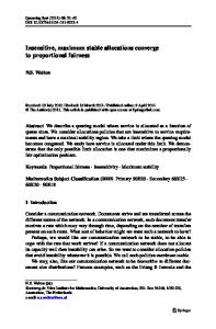
When Sj (·|φ) lies strictly above (below) Sj∗ on the interior (0, 1), this implies φ is excessive everywhere (nonviable everywhere). Realistically, we should expect that most viable restraints are at least somewhat excessive. For example, if we restrict attention to restraints such that the payoff function Sj (·|φ) is “well-behaved,” then every RDF φ will be either perfectly proportional, excessive everywhere, or nonviable everywhere. And φ∗ is the knife-edge separating the latter two categories. Proposition 2. For any RDF φ, (i) Sj (·|φ) is linear if and only if φ = φ∗ (perfectly proportional). (ii) If Sj (·|φ) is strictly concave, then φ > φ∗ on (0, 1) (excessive everywhere). (iii) If Sj (·|φ) is strictly convex, then φ < φ∗ on (0, 1) (nonviable everywhere). Proof. Appendix. Figure 1 illustrates the results in Proposition 2. The figure shows a challenger’s payoff associated with four different RDFs: the perfectly proportional restraint, φ∗ ; an RDF that is nonviable everywhere, φN V ; and two distinct kinds of excessive restraints, φIP and φA . Challenger’s Profit

Sj∗ (σ)

Sj (σ|φIP ) Imperfectly Proportional

∗ πN

Sj (σ|φA ) Accommodating

Sj (σ|φN V ) Nonviable

σ

Figure 1: Challenger Payoffs for Different RDF Categories.

Figure 1 illustrates an important point about the perfectly proportional RDF: it is the only RDF that is viable everywhere, but never excessive. As such, it should be regarded

19

as a theoretical optimum, but not something an antitrust regime can realistically demand in practice. Instead, we advocate a more practical approach. First, we categorize all excessive restraints into two types, with one type (“imperfectly proportional”) that at least approximates a perfect restraint, while the other type (“accommodating”) are much more problematic. In Figure 1, these two types correspond to the RDFs φIP and φA . We can then identify what types of restraints are likely to map to RDFs in either category. Definition 10. Let φ be excessive. Then φ is imperfectly proportional if Sj (·|φ) is strictly decreasing whenever positive-valued. Alternatively, φ is accommodating if ∗ Sj (·|φ) is nonmonotonic with maxσ Sj (σ|φ) > πN . Both of these categories have low exclusion rates (i.e. below ψ ∗ ), at least at low σvalues. What distinguishes the accommodating case is that there is a range of σ-levels at which the exclusion rates are negative, reflecting that Sj (·|φ) is initially increasing in σ. This means that the challengers actually want to be restrained to some positive degree. The result is that every σ 0 < arg maxσ Sj (σ|φ) is Pareto-dominated. We address these two restraint classes in the subsections that follow.

2.4.1

Imperfect Proportionality

An imperfectly proportional RDF maintains the desirable property that challengers always want σ to be as small as possible. As such, it exhibits a hallmark feature of perfectly proportional restraints, which is that lower values of θ always map into lower σ-values. As such, these restraints can at least provide a reasonable approximation of the perfect case. The eponymous imperfections are the result of a persistently low average exclusion rate. The result is that, while the perfectly proportional restraint has the property that C(θ|φ) = {θ}, imperfectly proportional ones give rise to non-singleton bargaining cores. Further, because these RDFs generate monotonic payoffs for all firms, they are viable at all points at which φ lies weakly above φ∗ . Proposition 3. Let φ be imperfectly proportional. Then (i) θ ∈ Vφ if and only if φ(θ) ≥ φ∗ (θ) (ii) θ < σe0 (θ|φ) < σej (θ|φ) 20

Proof. Appendix. The first condition ensures that Vφ consists in the points at which Sj (·|φ) lies weakly above Sj∗ .37 The second condition says that there is bargaining over an interval of σlevels, but this interval does not include the perfectly proportional magnitude σ = θ (at least not unless litigation costs are sufficiently large). If we allowed for positive litigation costs, our analysis implies that depending on litigation costs and the distribution of bargaining power, it may be impossible to garner a proportional settlement (σ = θ) if the parties use an excessive restraint. Nevertheless, the distance between θ and the bargaining core may be arbitrarily small, and we can rank imperfectly proportional restraints in terms of how far the core’s endpoints lie from θ. To do so, we rely on the following ordering. Definition 11. φa is more proportional than φb if φa (σ) ≤ φb (σ) whenever φa (σ) ≥ φ∗ (σ). And φa is strictly more proportional if the inequality is strict whenever φb (σ) > φ∗ (σ). In words, φa is more proportional than φb if, whenever φa permits excessive profits, φb also does so, and to a larger degree. It is straightforward to show that, given two imperfectly proportional restraints, if one is more proportional than the other then it will generate bargaining cores that come closer to θ. Proposition 4. Let φa and φb be excessive everywhere and imperfectly proportional. If φa is strictly more proportional than φb then, for any θ ∈ (0, 1), σe0 (θ|φa ) < σe0 (σ|φb ) and σej (θ|φa ) < σej (σ|φb ). Proof. Appendix. We can use this to compare specific kinds of restraints—say, z and y—in terms of proportionality. In particular, if two restraints z and y affect equilibrium behavior in the same way—but with y generating larger payoffs for challengers at every level of industry profits—then z must elicit a more proportional RDF, provided that both restraints are viable. This is sufficient to show that royalties (or two-part tariffs) are always more proportional than output caps or price floors. If φ were accommodating (and not globally concave or convex), then Sj (·|φ) could cross Sj∗ (·) from below, so if challengers refuse σ = θ they may still accept some larger σ 0 > θ. 37

21

Proposition 5. Fix two restraints z and y that perturb a common game G, with component functions zi (x, α) and yi (x, β), where α ∈ [0, α] and β ∈ [0, β]. Suppose that both restraints are viable everywhere, and that the following obtain for all interior σ: (i) xz∗ (αz (σ)) = xy∗ (βy (σ)) (ii) zi∗ (αz (σ)) > yi∗ (βy (σ)) for all i Then, φz is strictly more proportional than φy . Proof. Appendix. Intuitively, both royalties and output caps raise joint profits by reducing challengers’ output, which is captured generally in condition (i) above. However, a royalty imposes a cost on challengers, so that zj∗ (α) > 0 for interior α. By contrast, the restraint function yj representing an output cap has yi∗ (β) = 0 for all i, since the cap is merely a contractual obligation prohibiting challengers from setting their output above a given threshold. There is no “cost” imposed on the challengers. Instead, the impact on challengers’ profits comes entirely from distorting the equilibrium profiles x∗y (·). We illustrate this with an example below, which applies an output cap to the same environment in which we modeled a royalty in example 2. The output cap performs strictly worse: it is either imperfectly proportional or accommodating, depending on n. Example 4 (Output Caps in Linear Cournot). Consider the same linear Cournot model from example 2. But now the restraint is a cap on challengers’ sales. The unrestrained equilibrium involves all firms choosing output level x∗ = 1/(n + 2). An output cap is a parameter α ∈ [0, x∗ ] such that each j is constrained to set xj ≤ x∗ − α. P The restraint functions are zj (x, α) = 1{xj > α}D and z0 = j zj , where D is a prohibitively expensive penalty for breaking the cap agreement. The average exclusion rate is ψ(σ|φz ) =

2n(n + 2)αz (σ) − 2(n − 2) 2n2 − (n + 2)n2 αz (σ)

It is easy to verify that ψ(σ|φz ) < n42 = ψ ∗ for all αz (σ) < x∗ ≡ α, and hence φz is excessive. Moreover, when n ≥ 3, ψ(σ|φz ) < 0 for some low range of σ-values, so Sj (·|φ) is initially strictly increasing. Hence φz is accommodating when n ≥ 3, and imperfectly proportional when n ≤ 2. 22

2.4.2

Accommodating Restraints

Accommodating restraints are characterized by nonmonotonicity of Sj (·|φ) such that challengers actually want to be restrained with some nonzero magnitude. In all examples we have identified, Sj (·|φ) is strictly concave, at least whenever it is nonzero valued. There are two reasons that a restraint can be accommodating. The first is that its effect of diminishing competition between challengers may initially dominate its effect of giving the patentee a competitive advantage. This was illustrated in example 4. Intuitively, as the cap becomes increasingly stringent, the challengers start to behave exactly like a smaller number of firms would have behaved in a more concentrated market. So, for example, at some cap level, the n challengers behave like a single duopolist in a more concentrated market, and this is profitable when n is sufficiently large. In fact, the challengers’ profit-maximizing σ-level is that which replicates a Stackelberg duopoly, with the challengers acting collectively as the leader.38 However, as the example below illustrates, this Stackelberg-replicating property is not necessary for a restraint to be accommodating. Example 5 (Territorial Restraints with Divided Challengers). Consider the territorial restraint in example 3 (which was perfectly proportional). But now suppose the patentee partitions the challengers’ territory, [α, 1], into n sub-regions of length (1 − α)n−1 . Thus, [α, 1] comprises n “little duopolies,” each between the patentee and ∗ one challenger. Each challenger’s profit (1 − α)n−1 π2∗ . If π2∗ > nπN , then we must have ∗ −1 ∗ (1 − α)n π2 > πN for sufficiently small α, and hence the restraint is accommodating. One major problem with accommodating restraints is that they lead some low σ-levels to be Pareto-dominated by larger ones. Definition 12. Conditional on an RDF φ, a magnitude σ is Pareto-dominated if there exists σ 0 6= σ such that SI (σ 0 |φ) > SI (σ|φ) and Si (σ 0 |φ) ≥ Si (σ|φ) for all i. A σ-level can be Pareto-dominated only when Sj (·|φ) is not strictly monotonic. In particular, if Sj (·|φ) is nondecreasing at σ, then σ must be Pareto-inferior. So, for example, in the restraint φA in Figure 2, all σ ∈ [0, σ peak ] are Pareto-dominated, where σ peak is the magnitude at which Sj (·|φA ) attains its peak value. 38

This requires that the challengers’ combined output in the unrestrained equilibrium exceeds that which would be chosen by the leader in a Stackelberg-duopoly.

23

One might expect that price restraints—floors on challengers’ price-levels—are equivalent to output caps. But in fact price floors are worse. Both restraint types generate a Pareto-dominated range of low σ-values, since Sj is initially strictly increasing. But the output cap approximates an imperfect restraint at high σ-values (as illustrated in Figure 2), while the price restraint creates additional problems at this range. In particular, φ(σ) falls to zero at an interior point σ φ=0 < 1, so Sj (·|φ) eventually crosses Sj∗ (·) from above, hitting zero at σ φ=0 . This reflects that, even when the price floor is sufficiently large to exclude challengers, it is not necessarily large enough to permit monopoly pricing by firm 0.39 Challenger’s Profit

Sj (σ|φA ) Accommodating

Sj∗ (σ)

∗ πN

σ peak

σ φ=0

σ

Pareto-Dominated Regions

Figure 2: Accommodating RDF with Two Regions of Pareto-Dominated σ-levels.

Thus the patentee engages in limit pricing over the interval [σ φ , 1), over which range Sj is flat and equal to zero. Consequently, this range of magnitudes is Pareto-dominated, and φ is nonviable within it.40 The example below depicts a price floor in a Hotelling duopoly, and the corresponding graph of Sj (·|φ) is illustrated in the figure below.41 39

Monopoly is not attained until σ = 1, so firm 0 is not setting a monopoly price in the limit σ → σ φ=0 . If it tried to set a monopoly price here, challengers would be able to enter and make profitable sales. R1 40 Recall that 0 ψ(σ|φ)dσ = ψ ∗ for all φ (Corollary 2). Since ψ(·|φ) is initially negative for an accommodating restraint, it must eventually exceed ψ ∗ by a discrete amount. Relative to an output cap, a price floor undergoes this transition in more exaggerated fashion: ψ(·|φ) is initially more negative, and later exceeds ψ ∗ by much more—to the point that the restraint becomes nonviable in a left-neighborhood of unity. 41 The fact that the restraint is accommodating even though n = 1 is due to conjectural variation: even in duopoly, a Bertrand firm wants to commit to a less competitive strategy.

24

Example 6 (Price Restraints in a Hotelling Duopoly). There is one consumer at each location l ∈ [0, 1]. Firm 0 (firm 1) is at location l = 0 (l = 1). Each firm i sets a price pi . A consumer l gets surplus 1 − 14 l − p0 (1 − 14 (1 − l) − p1 ) if it buys from firm 0 (firm 1, the only challenger). With costless production, monopoly involves ∗ = 12 , pm = 43 , q m = 1, and π m = 43 , while the unrestrained equilibrium yields p∗N = 41 , qN ∗ = 14 . Firm 0 imposes a price floor such that firm 1 must set p1 ≥ p∗N + α.42 and πN Equilibrium payoffs are    1 [1 + 2α]2

if α <

 1 [1 + 2α]

if

u∗0 (α|z) =  8 4

1 2

1 2

≤α≤1

   1 [1 − 2α][1 + 4α]

u∗1 (α|z) =  8 0

if α < if

1 2

1 2

≤α≤1

Firm 1 is fully excluded at α ≥ 12 , but firm 0 does not acquire the monopoly profit until α = 1. Thus all α ∈ [ 12 , α) are Pareto-dominated. Firm 1’s payoff is strictly increasing when α < 41 , with a maximum at α = 18 . Thus the restraint is accommodating, and all α ∈ [0, 18 ) are Pareto-dominated. The second reason a restraint may be accommodating is that it may generate very strong strategic effects that make the patentee behave much less competitively. This can happen when the restraint gives the patentee a strong financial interest in the challengers’ commercial success. We illustrate this with an example in which the challengers pay for licensing rights with shares of stock, effecting a partial acquisition of each challenger. Example 7. Consider the same Cournot model as in examples 2 and 4. The restraint involves the patentee acquiring an ownership share α in each challenger, giving it this fraction of each j’s profit.43 The marginal exclusion rate is ψ(σ|φz ) =

nαz (σ) − (n − 2) n2 [1 − αz (σ)]

n+2 n+2 This yields ψ(σ|φz ) < ψ ∗ = 4/n2 (ψ(σ|φz ) > ψ ∗ ) whenever α < n+4 (α > n+4 ), so the restraint is excessive. Moreover, ψ(·|φz ) is initially negative when n ≥ 3. Thus φz is accommodating in this case, but imperfectly proportional when n ≤ 2. 42 43

Restraint functions are analogous to those in example 4. P Thus the restraint functions are zj (x, α) = απj (x) and z0 = j zj .

25

2.5

Side-Deals

At least two kinds of “side-deals” always act to destroy proportionality, no matter what kind of restraint they accompany. The first is a reverse payment: a payment from the patentee to the challengers. The second is a countervailing restraint: a separate restraint imposed on the patentee. In fact, the two are largely equivalent, with the only difference being that the former elicits monopoly, while the latter effects a cartel.

2.5.1

Reverse Payments

A fixed license fee is a lump sum τ > 0 paid by each challenger to the patentee, and will never raise antitrust concerns.44 By contrast, reverse payment (values τ < 0) are deeply concerning. If they are allowed, then the firms can always redistribute total profits however they like through transfers. Then, since monopoly maximizes total profits, the following result is immediate: Proposition 6. Suppose the firms can choose any reverse payment τ < 0. Then, for any φ, every σ < 1 is Pareto-dominated. This clarifies the function and purpose of reverse payments: to subvert proportionality. It also clarifies that there is no good reason to associate reverse payments with pay for delay. First, reverse payments destroy proportionality no matter what type of restraint they accompany. Second, we showed that delayed challenger entry—the restraint type in pay for delay—is perfectly proportional when unaccompanied by a reverse payment.

2.5.2

Countervailing Restraints on the Patent Holder

Countervailing restraints imposed on the patentee soften the blow of the restraint imposed on challengers, since the patentee gains a smaller competitive advantage. And, indeed, restraining all competitors in parallel is the basic ingredient in a cartel. It is thus easy to see how countervailing restraints can destroy proportionality. For example, consider the territorial restraint from example 3, but with n = 1. However, now suppose that the patentee agrees to stay out of the challenger’s territory, [α, 1]. Clearly 44

This manner of financing does not restraint competition, after all.

26

this is just ordinary market division, and industry profits will always be π m . Similarly, it is well known in the economic literature on licensing that rivals could charge each other royalties in order to facilitate the same results as express price fixing (Shapiro, 1985). This is easy to formalize using our model. Continue to assume that the firms bargain over σ, which determines the size of industry profits, Π(σ). But now the patentee will itself be restrained—in the same way as the challengers, but not necessarily to the same degree—so that any level of Π(σ) will be distributed differently. We can thus model a countervailing restraint as a magnitude γ ∈ [0, 1] such that, for each σ, a challenger’s industry profit share rises from φ(σ) to Φφ (σ, α), where Φφ (σ, α) ≡ γ

1 + (1 − γ)φ(σ) N

And payoff functions are thus S0 (σ, γ|φ) ≡ [1 − nΦφ (σ, γ)]Π(σ) and Sj (σ, γ|φ) ≡ Φφ (σ, γ)Π(σ). It is easy to see that, just like reverse payments, countervailing restraints will always destroy proportionality. Proposition 7. Suppose the firms can choose any countervailing restraint γ ∈ [0, 1]. Then, for any φ, every σ < 1 is Pareto-dominated. Proof. Fix γθc such that Φφ (1, γθc )π m = Lcj (θ). Then S0 (α, γθc |φ) = π m − nLcj (θ) > LcI (θ) − nLcj (θ) = Lc0 (θ). Then (σ, γ) = (1, γθc ) is mutually-acceptable, and it Paretodominates every (σ 0 , γ 0 ) with σ 0 < 1.

2.5.3

A Note on Multi-Patentee Settlements

In practice, many horizontal settlements involve several patentees, each wanting to use the others patents. In this case, we would expect that the patents are themselves complementary, although the firms sell competing products. It is well understood that patent pooling is an efficient way to license complementary, separately-held patents, since it eliminates a double marginalization problem (Lerner and Tirole, 2004). Alternatively, the firms might just cross-license with each other. It is beyond the scope of this paper to explore multi-patentee settlements comprehen27

sively. But our conclusions about countervailing restraints enable us to make at least one important point, which is that these settlements can create serious antitrust concerns if all firms are restrained. There must be at least one unrestrained competitor in order to keep the firms honest. And, intuitively, it is never necessary for all firms to be restrained in order to support a viable settlement.45 There must be one patentee who contributes weakly more (in terms of the value and quality of his patents) than the others. This is the patent holder who would expect the largest post-judgment profits if all patents were litigated.46 Like firm 0 in our single-patentee settlements, this firm need not be restrained at all, although it may be necessary for some or all of the others to be restrained.

3

Antitrust Analysis

Our proposal would have antitrust look first to the nature of the restraint imposed on challengers. As a guiding principle, the most important question is whether we can expect that the challengers always want the restraint’s magnitude to be as small as possible—even if they are all restrained in parallel. Based on our analysis, some restraints are likely to be at least approximately proportional under most or all market conditions. These include royalties, pure delay,47 and nonexclusive territorial restraints in which challengers are not contractually separated. Such restraints might not be literally perfectly proportional, but it is hard to imagine any circumstances in which they would not be at least imperfectly proportional in the sense that challenger’s always want to be restrained as little as possible. Other restraint types are more problematic, and will virtually always be excessive, although they may not always be accommodating. For instance, when a patent dispute is resolved by concentrating firm ownership in one way or another, as in the stock acquisition example, the settlement presents a serious threat to competition, although here the concerns are fairly obvious. Restraints on output or price are similarly problematic, 45

A caveat is that, in practice, if there are many firms (not necessarily all competitors) pooling their patents, transaction costs could be high enough to justify an arrangement in which everyone pays royalties to the pool. 46 If no patent holder is the leader in this sense, then none of them need be restrained. 47 As noted in an earlier footnote, pure delay still be problematic in pharmaceutical markets, due to the problematic results of certain badly-drafted provisions in the Hatch-Waxman Act.

28

with the latter generally being more problematic than the latter. In these cases, the restraints may be accommodating in the sense that they can enhance challengers’ profits by softening the extent to which they compete with each other. As such, it is important to determine whether the challengers know they are being restrained in parallel. But even if they are not, these restraints are still often problematic by virtue of having low exclusion rates. Despite our results, it may be reasonable for a settlement to involve both an output cap and a royalty, however. One problem with royalties is that, realistically, it would be hard for firms to predict its output effects with precision. But an output cap is always precise, and if it is accompanied by a nontrivial royalty obligation, it is likely to be reasonably proportional. Aside from looking at the restraint type, antitrust must look for the kinds of problematic side-deals that we have discussed. Reverse payments are an obvious example. These should not be viewed as specific to pay for delay, but should rather be regarded as a universal threat to proportionality. Indeed, as we showed, they always subvert proportionality, no matter what kind of restraint they accompany. Similarly, antitrust should be very suspicious of countervailing restraints on the patentee, which is very similar to a reverse payment in the sense that it persuades challengers to be further restrained themselves. In settlements with multiple patent holders, we can say something similar, which is that at least one of the patent holders should not be restrained. This is critical to keep the firms honest.

3.1

A “Hub and Spoke Test” for Accommodating Restraints

Accommodating restraints can replicate what the antitrust literature calls a “hub and spoke” conspiracy.48 Traditionally this involves all competitors in a market (the “spokes”), who cannot directly coordinate due to antitrust, but who try to accomplish an identical result indirectly. Every spoke writes an identical bilateral agreement with a common partner (the “hub”), which operates in a vertically-related market. In all of the bilateral contracts, the hub imposes the same restraint on one of the challengers, so the cumulative effect is identical to direct collusion. But the hub is assumed not to have the power to force these restraints on the spokes of its own volition; the spokes 48

The best-known case is Interstate Circuit, Inc. v. United States, 306 U.S. 208 (1939).

29

could avoid them if they wanted. An accommodating restraint can be similar, for the challengers may benefit from being restrained in parallel, even if they could credibly demand a weaker restraint. We can use this analogy to construct an intuitive, nontechnical test for deciding whether a given kind of restraint is likely to be accommodating. The test is as follows: take a given settlement, but suppose that the patentee were a market outsider rather than a competitor. Then ask whether the challengers might benefit from being restrained in parallel by the outside patentee (relative to being unrestrained). It is easy to see why things like royalties or pure delay will not be accommodating. A group of competitors would never benefit from having an outsider double-marginalize all of them in parallel. On the other hand, it is obvious that the firms could benefit from an outsider imposing parallel price or output restraints on them. Similarly, in the case where the patentee acquires shares of stock in the challengers, this could benefit the firms by facilitating common ownership and thereby softening competition.

3.2

Challenger Coordination

A separate settlement for each challengers necessarily multiplies the requisite transaction costs. Further, even if we think a restraint type is perfectly reasonable, a challenger may have reasonable concerns about potentially being more restrained than other challengers, and this could lead to bargaining breakdowns. On the other hand, for exceedingly obvious reasons, coordination among competing challengers presents antitrust concerns. Perhaps the simplest principle antitrust espouses is that bad things can happen when competing firms coordinate on terms that restrain them in parallel. But in fact there may be cases in which it is reasonable—or even efficient—to let challengers coordinate. In particular, if we are absolutely satisfied that a particular restraint type is appropriately proportional, then there may be no clear downside to letting the challengers bargain collectively against the patentee. A proportional restraint (even if imperfect) always has the property that challengers want to be restrained as little as possible. So there is no risk that they will accept a more restrictive settlement than they could credibly demand. And this would substantially diminish transaction costs and other contracting problems that might otherwise arise.

30

4

Conclusion

Competitors can and do settle patent disputes or challenges in many different ways, and the resulting competitive effects vary widely in the extent to which they line up with the firms’ true expectations about litigation outcomes. This paper advocates a standard under which antitrust’s general objective is to limit firms to proportional settlements, or those in which total profits resemble what the firms believe they would get (in expected value) from litigation. Our contribution is to demonstrate the conditions under which this arises naturally through markets and private contracting, so that the firms’ settlements necessarily reflect the firms true beliefs about patent quality and litigation odds. We show that one can make strong inferences about a settlement’s proportionality by simply looking at the nature of the agreement: the manner in which competition is restrained, and certain “side-deals” that always subvert proportionality. As such, this approach does not require estimating competitive effects or the expected outcome of counterfactual patent litigation.

5

References

Bessen, James E and Michael J Meurer (2006) “Patent litigation with endogenous disputes,” The American economic review, pp. 77–81. Carrier, Michael A. (2012) “Why the ‘Scope of the Patent’ Test Cannot Solve the Drug Patent Settlement Problem,” Stanford Technology Law Review, Vol. 61, pp. 1–8. Choi, Jay Pil (2005) “Live and let live: A tale of weak patents,” Journal of the European Economic Association, Vol. 3, pp. 724–733. Daughety, Andrew F and Jennifer F Reinganum (2005) “Economic theories of settlement bargaining,” Annu. Rev. Law Soc. Sci., Vol. 1, pp. 35–59.

31

Dolin, Gregory (2011) “Reverse Settlements as Invalidity Signals,” Harvard Journal of Law and Technology, Vol. 24, pp. 281–333. Edlin, Aaron, Scott Hemphill, Herbert Hovenkamp, and Carl Shapiro (2015) “The Actavis Inference: Theory and Practice,” Rutgers UL Rev., Vol. 67, p. 585. Farrell, Joseph and Robert P Merges (2004) “Incentives to challenge and defend patents: Why litigation won’t reliably fix patent office errors and why administrative patent review might help,” Berkeley technology law journal, pp. 943–970. Farrell, Joseph and Carl Shapiro (2008) “How strong are weak patents?” The American Economic Review, Vol. 98, pp. 1347–1369. Helland, Eric and Seth A Seabury (2016) “Are Settlements in Patent Litigation Collusive? Evidence from Paragraph IV Challenges,”Technical report, National Bureau of Economic Research. Hemphill, C Scott (2006) “Paying for delay: Pharmaceutical patent settlement as a regulatory design problem,” NYU Law Review, Vol. 81, p. 1553. Hemphill, C Scott and Mark A Lemley (2011) “Earning Exclusivity: Generic Drug Incentives and the Hatch-Waxman Act,” Antitrust Law Journal, Vol. 77, pp. 947– 989. Hopenhayn, Hugo, Gerard Llobet, and Matthew Mitchell (2006) “Rewarding sequential innovators: Prizes, patents, and buyouts,” Journal of Political Economy, Vol. 114, pp. 1041–1068. Hovenkamp, Erik (2016) “Challenge Restraints and the Scope of the Patent,” Antitrust Chronicle, Vol. 1, pp. 46–55. Hovenkamp, Erik and Jorge Lemus (2016) “Reverse Settlement and Holdup at the Patent Office.” Hovenkamp, Herbert, Mark Janis, and Mark A Lemley (2002) “Anticompetitive settlement of intellectual property disputes,” Minn. L. Rev., Vol. 87, p. 1719. Kesan, Jay P and Gwendolyn G Ball (2006) “How Are Patent Cases Resolved-An Empirical Examination of the Adjudication and Settlement of Patent Disputes,” Wash. UL Rev., Vol. 84, p. 237. 32

La Belle, Megan M, “Against Settlement of (Some) Patent Cases,” VANDERBILT LAW REVIEW, Vol. 67, p. 375. Lemley, Mark A and Mark Pl McKenna (2016) “Scope,” Wm. & Mary L. Rev., Vol. 57, p. 2197. Lemley, Mark A and Carl Shapiro (2005) “Probabilistic patents,” The Journal of Economic Perspectives, Vol. 19, pp. 75–98. Lerner, Josh and Jean Tirole (2004) “Efficient patent pools,” The American Economic Review, Vol. 94, pp. 691–711. Maurer, Stephen M and Suzanne Scotchmer (2006) “Profit neutrality in licensing: The boundary between antitrust law and patent law,” American Law and Economics Review, Vol. 8, pp. 476–522. Meurer, Michael J (1989) “The settlement of patent litigation,” The RAND Journal of Economics, pp. 77–91. Nordhaus, William D et al. (1967) “The optimal life of a patent,”Technical report, Cowles Foundation for Research in Economics, Yale University. Olson, Luke M and Brett W Wendling (2013) “Bureau of Economics Federal TRade Commission Washington, DC 20580.” Scott Morton, Fiona and Carl Shapiro (2016) “Patent Assertions: Are We Any Closer to Aligning Reward to Contribution?” Innovation Policy and the Economy, Vol. 16, pp. 89–133. Shapiro, Carl (1985) “Patent Licensing and R&D Rivalry,” American Economic Review, Vol. 75, pp. 25–30. (2003) “Antitrust limits to patent settlements,” RAND Journal of Economics, pp. 391–411. Spier, Kathryn E (2007) “Litigation,” Handbook of law and economics, Vol. 1, pp. 259–342. Willig, Robert D and John P Bigelow (2004) “Antitrust policy toward agreements that settle patent litigation,” Antitrust Bull., Vol. 49, p. 655.

33

Appendix Proof of Proposition 2 Proof. For part (i), note that Sj∗ is a linear functions of σ. Given that for any restraint φ ∗ and Sj (1|φ) = 0, if Sj (·|φ) a challenger’s profit is fixed at two points, i.e., Sj (0|φ) = πN ∗ is linear then it must be that φ = φ∗ . For part (ii), using the fact that Sj (0|φ) = πN and N Sj (1|φ) = 0 plus the definition of strict concavity we have Sj (σ|φ) > (1 − σ)π which implies φ > φ∗ . Part (iii) is analogous to part (ii). Then note that strict concavity (strict convexity) implies Sj (·|φ) lies strictly above (strictly below) Sj∗ over the interior (0,1), implying φ is excessive everywhere (nonviable everywhere).

Proof of Proposition 3 Proof. For part (i), fix θ ∈ (0, 1), and let σei = σei (θ|φ) for each i = 0, j. Note that Si (σei |φ) = L0i (θ) for all i. We have θ ∈ Vφ if and only if Π(σej ) ≥ Π(θ) (or σej > θ because Π(·) is strictly increasing). Then, because Sj (·|φ) is strictly monotonic, we have θ ∈ Vφ ⇐⇒ σej ≥ θ ⇐⇒ Sj (θ|φ) ≥ Sj (σej |φ) = Sj (θ|φ∗ ) ⇐⇒ φ(θ) ≥ φ∗ (σ) For part (ii), note that σ ∈ Int(Vφ ) implies σej > θ, since φ is excessive. Then φ(θ) > φ∗ (θ) implies S0 (θ|φ) < S0 (θ|φ∗ ) = L00 (θ), and hence σe0 > θ. To complete the proof, note that S0 (σej |φ) = Π(σej ) − nSj (σej |φ) = Π(σej ) − nL0j (θ) > Π(θ) − nL0j (θ) = L00 (θ) = S0 (σe0 |φ) which implies σe0 < σej by monotonicity.

Proof of Proposition 4 Proof. Fix θ. Let σeik = σei (θ|φk ) for each i ∈ {0, j} and k ∈ {a, b}. Then Sj (σeja |φa ) = L0j (θ) = Sj (σejb |φb ) ≥ Sj (σejb |φa ) 34

which implies σeja ≤ σejb . A symmetric argument shows σe0a < σe0b .

Proof of Proposition 5 Proof. Recall that, when the game is restrained, payoff functions are u0 (x|α, z) = π0 (x) + z0 (x, α) and uj (x|α, z) = πj (x) − zj (x, α) for each j, with the equilibrium values of each ui and zi denoted u∗i (α|z) and zi∗ (α). From condition (i), we have     πi xz∗ (αz (σ)) = πi xy∗ (βy (σ)) for all σ. Then, using condition (ii), the following obtains for all interior σ: u∗i (αz (σ)|z) < u∗i (βy (σ)|y) for all i ⇐⇒ Sj (σ|φz ) < Sj (σ|φy ) ⇐⇒ φz (σ) < φy (σ) Then, given that φz and φy are viable, φz is strictly more proportional than φy .

Online Appendix 5.1

Proportionality with Fixed-Term Patents

How could we hope to achieve proportionality in a system where all patents get the same twenty years of protection? As a heuristic, suppose the Patent Office employed a perfectly-informed patent examiner who could optimally assign “fine-tuned” terms to every new invention, so as to maximize dynamic welfare. Conditional on the prior art, it gives an invention x a custom term length, τ ∗ (x), with more innovative inventions getting a longer term. We can thus regard τ ∗ (x) as an ordinal measure of patent quality. As such, we can interpret a fixed-term system as one that stipulates a quality threshold τb such that x is patentable if and only if τ ∗ (x) ≥ τb, and then gives a common term T (which we take to be twenty years) to all patentable inventions.49 49

We can think of τb as further determining how much “territory” a patentee can claim around a particular embodiment of her invention—the “scope” of the patent—although we will not model scope explicitly. See Lemley and McKenna (2016) for a discussion of the connection between validity and scope.

35

The optimal fixed term must satisfy τb < T because, if τ ∗ (x) is just slightly below T (so that the invention deserves almost twenty years), it must be better to give a slightly excessive term than no protection at all. However, virtually all inventions in the fixedterm system (namely any for which τ ∗ (x) 6= T ) will not have an optimal term length. This is reflected in the figure below, which shows the deviations of the fixed term from the fine-tuned terms that would be assigned to inventions spanning a range of different quality levels. Term Length Granted T

B2 B3

E1 E2 B1 T

τb

τ ∗ (x)

Figure 3: Deviations of the fixed term, T , from the optimal ones, τ ∗ (x).

Invention quality τ ∗ (x) is the x-axis variable, while the y-axis corresponds to term length. A perfect examiner office would assign the terms corresponding to the dashed 45 degree line. By contrast, in the fixed-term system, only inventions with τ ∗ (x) ≥ τb are patentable. Even ignoring granting errors, the fixed-term system gives some inventions too much protection, but others too little. Area B1 represent inventions that get zero years of protection instead of τ ∗ > 0. These are not errors of the patent office, but instead an inefficiency imposed by constraining the patent office to be a binary system. Area E1 , instead, represents errors of an imperfect patent office. These are inventions that deserve less than τb years of patent protection but they obtain T years of protection by mistake. Similarly, areas B2 and B3 represent suboptimal patent length due to the binary constraint of patent system, whereas area E2 patent office errors by rejecting patent applications that deserve more than τb years of protection. Appendix 5.2 considers a patent system in which patents are “probabilistic” in the sense that private parties are generally uncertain as to how a court would apply the general 36

standards of patentability to a specific patent.50 The analysis shows the conditions under which patentability laws yield just the right amount of uncertainty in a given case—the patentee’s expected payoff from litigation (ignoring litigation costs) equals the optimal reward for the invention. Under this condition, private settlements of patent challenges elicit optimal rewards to the extent that settlement profits line up with the expected payoffs from litigation. In such cases, challenge threats and the ensuing settlements can approximate the fine-tuning function performed by the hypothetical perfect patent office, at least for those inventions that receive patents.51 A perfect patent office achieves parity between contributions and rewards that maximize social welfare by granting exclusion rights not vulnerable to challenges (there are no mistakes). By contrast, an imperfect fixed-term system achieves it by relying on challenge threats and private contracting to “soften” the patent’s market footprint to a degree that is commensurate with the probability of invalidity. To resolve validity challenges, the patentee can offer rivals some restrained access to the invention, such as a right to make a certain capped number of licensed sales. The higher the likelihood of invalidity, the weaker the restraint the patent holder can demand. As such, although all patents still get twenty years of protection, differences in patent quality elicit variability in the extent to which competition is diminished. Figure 4 (left-hand graph) shows the reward that a patentee receives by obtaining monopoly profit flow (π m ) over the fine-tuned term τ ∗ (x), which is less than the fixed term T awarded in our binary patent system. Figure 4 (right-hand graph) shows the same patentee in a fixed-term system. Here the prospect of patent challenges softens the patent’s exclusionary effect, leaving the patentee with a smaller profit flow, π(θ), over the longer fixed term, T . In both graphs, the patentee’s profits fall to the competitive ∗ level, πN , after the patent expires. When τ ∗ (x)π m = T π(θ) the patentee’s reward is the same in both cases (shaded areas measure the same). This is how a fixed-term patent system can achieve proportionality. 50

The notion of “probabilistic patents” was introduced in Lemley and Shapiro (2005). A fixed term system cannot elicit proportional rewards for minor inventions that fall short of the law’s patentability threshold, but which would have received a small but nonzero term from a perfect patent office. 51

37

Profit Flow

Profit Flow

πm

πm π(θ)

πN

πN

τ ∗ (x)

time

τ ∗ (x)

T

time

Figure 4: The shaded areas represents the reward of an invention. The left figure shows a perfect patent system and figure on the right shows a binary patent system where a challenge brings the expected payoff to π(θ). The shaded areas are of the same size.

5.2

Optimal Rewards via Litigation Expectations

Let τ ∗ (x) be the patent term function defined in Section 2. We now show that a fixed term patent system can elicit expected litigation payoffs (ignoring litigation costs) that provide optimal rewards for the patented inventions. Our underlying assumption is that firms are not perfectly informed as to how a court will apply the general standards of patentability to the specific patent in suit. This embodies the notion of “probabilistic patents” introduced by Lemley and Shapiro (2005). The authors note that there is “considerable uncertainty about [a patent’s] validity and scope,” and that such uncertainty would still exist “even if the process for granting patents [were] improved.” We will therefore model patent law as assigning probabilities of validity to all granted patents, with higher invention quality (larger τ ∗ (x)) translating into higher patent quality. Conditional on τb, a court evaluating a patent’s validity will base its decision on a noisy signal of patent quality, y(x) ∼ F (y|x) commonly known among firms. The probablity that a patent is deemed valid is therefore 1 − F (y|x). We assume the patent office is imperfect but unbiased. That is, although the patent office makes mistakes, for a given patentability threshold the office is unbiased. In other words, we make the following assumption: Ey [F (y|x)] = F (τ |x). With that, the expected probability of validity, which we define as the patent quality, is given by θbτ (x) ≡ 1 − F (τb|x)

38

(8)

A fixed-term patent system can approximate the ideal proportionality that would accrue from perfectly fine-tuned patents. Following the notation from the main text, let π m (x) ∗ ∗ and πN (x) be the values of π m and πN corresponding to x. Ignoring litigation costs, conditional on signal realization y, the patentee’s expected payoff (over fixed term T ) from litigating to judgment at the beginning of the patent term is h





i

∗ θbτ (x)π m (x) + 1 − θbτ (x) πN (x) T

(9)

This payoff equals the payoff that the patentee would get—over the same period, T — if its patent had the fine-tuned term τ ∗ (x) if h





i

∗ (x) T τ ∗ (x)π m (x) + [T − τ ∗ (x)]π N (x) = θbτ (x)π m (x) + 1 − θbτ (x) πN

(10)

From this equation we obtain 1 − F (τb|x) =

τ ∗ (x) . T

When this condition is met, expected litigation payoffs (ignoring litigation costs) will give the patentee exactly the optimal proportional reward. This result has some nice properties. First, it does not depend on market structure terms, such as profit flows. Second, patent quality is equal to 1 whenever τ ∗ (x) ≥ T , and equal to 0 when τ ∗ (x) = 0. Thus, there is no uncertainty when either (1) the patent’s optimal fine-tuned term is exactly zero; or (2) the patent’s optimal term is at least twenty years. We can think of (1) to the case where the “invention” actually does not contribute anything new, given what is already known. Case (2) ensures that, if an invention really does warrant twenty years of protection, then the patent system will not diminish the patentee’s reward by creating uncertainty.

39