Properties of the Maximum q-Likelihood Estimator for Independent Random Variables Yoshihiko Hasegawa1∗and Masanori Arita1,2,3 1 Department

of Computational Biology, Graduate School of Frontier Sciences,

The University of Tokyo, Kashiwanoha 5-1-5, Kashiwa, Chiba, 277-8561, Japan 2 RIKEN

Plant Science Center, Suehiro-cho 1-7-22, Tsurumi-ku, Yokohama, Kanagawa 230-0045, Japan

3 Institute

for Advanced Biosciences, Keio University, Baba-cho 14-1, Tsuruoka, Yamagata 997-0035, Japan

Abstract In the last two decades, the nonextensive statistics proposed by Tsallis has been extensively discussed in terms of the Tsallis entropy, which is a generalization of the Boltzmann-Gibbs-Shannon entropy. Within the nonextensive framework, many kinds of generalizations have been made. Suyari (IEEE Trans. Inf. Theory 51 (2005) 753) has proposed the generalized likelihood called the q-likelihood, in which a traditional product operator is replaced by the q-product. We study properties of the maximum q-likelihood estimator (MqLE) which is a generalization of the conventional maximum likelihood estimator with the use of the q-likelihood. We discuss MqLE from the viewpoint of the minimization of the divergences in the nonextensive statistics. It has been shown that optimum parameters determined by the MqLE are nearly in agreement with those yielding the minimum distance of the divergence proposed by Rajagopal (Nonextensive Statistical Mechanics and Its Applications, 2000, p.99). We here show that the consistency of MqLE is achieved along with the nonnegativity of Rajagopal’s divergence. The asymptotic Gaussianity and robustness of the MqLE for independent random variables are discussed both by analytical methods and simulations.

Keywords nonextensive statistics, q-calculus, parameter inference, maximum likelihood estimation PACS 02.50.Cw; 02.10.-v; 05.90.+m ∗

Corresponding author : [email protected] (Yoshihiko Hasegawa)

1

1

Introduction

In usual systems consisting of n elements, physical quantities such as energy and entropy are proportional to n (extensive), and their thermodynamical properties in the equilibrium states are well accounted for by the Boltzmann-Gibbs statistics. In recent years, however, many efforts have been made for a study on nonextensive systems in which physical quantities are not proportional to n (nonextensive). This phenomenon is realized in complex systems such as a system with the long-range interaction and a system with nonequilibrium (quasi-equilibrium) states [1, 2, 3, 4]. In order to discuss the properties of nonextensive systems, Tsallis proposed the generalized entropy (called the Tsallis entropy) [5] defined by ˆ 1 − p(x)q dx Sq := , (1) q−1 where q stands for the entropic index and p(x) the probability density function (PDF). The Tsallis entropy reduces to the Boltzmann-Gibbs-Shannon entropy in the limit of q → 1 in Eq. (1). By using the Jayne’s maximum entropy principle (MaxEnt) [6] to the Tsallis entropy, we obtain the generalized distribution, for instance, q-Gaussian distribution [see Eqs. (51) and (52)]. Along with these generalizations, conventional arithmetic operators have also been generalized: q-exponential and q-logarithmic functions are generalization of the conventional exponential and logarithmic functions, respectively. These deformed operators are given by 1

expq (x) := [1 + (1 − q)x]+1−q , lnq (x) :=

x1−q − 1 (for x > 0), 1−q

(2) (3)

where [a]+ := max(0, a). It can be easily shown that lnq (x) is an inverse function of expq (x), and vice versa. Furthermore, q-product, which is a generalization of the arithmetic product, has also been proposed [7, 8] [Eq. (4)]: x ⊗ y := expq (lnq x + lnq y) q

=

[

x1−q + y 1−q − 1

1 ] 1−q

+

(for x > 0, y > 0).

(4)

Maximum likelihood estimator (MLE) is one of the most widely used parameter inference method. MLE gives the parameters at which likelihood functions have the maximum value. Let X = (X1 , X2 , · · · , XN ) be independent random variables sampled from PDF p(X; θ), x = (x1 , x2 , · · · , xN ) be their instances and θ be parameter (N is the number of samples). A likelihood and a log likelihood function of independent random variables for PDF p(X; θ) can be represented by Eqs. (5) and (6), respectively: 2

L(N ) (θ; x) :=

N ∏

p(xi ; θ),

(5)

ln p(xi ; θ).

(6)

i=1

L (N ) (θ; x) :=

N ∑ i=1

Suyari has proposed a q-likelihood [9, 10] function by replacing the “×” operators with “⊗q ” in the conventional likelihood function. This leads to ) L(N q (θ; x) := p(x1 ; θ) ⊗ p(x2 ; θ) ⊗ · · · ⊗ p(xN ; θ). q

q

(7)

q

(N )

If q = 1, Lq (θ) is identical to the conventional likelihood. Taking the q-logarithm [Eq. (3)] in the both sides of Eq. (7), we get q-log likelihood function given by Lq(N ) (θ; x)

:=

) lnq L(N q (θ; x)

=

N ∑

lnq p(xi ; θ).

(8)

i=1

MLE is a method to infer parameters by selecting the parameters which yields the maximum of likelihood functions. It is quite natural to think of the maximum qlikelihood estimator (MqLE), defined by θbq := argsup Lq(N ) (θ; x).

(9)

θ

Although in Ref. [9], Suyari has indicated that q-likelihood has connection with qGaussian distribution via the Gauss’ law of error, the properties of q-likelihood remain veiled. Because the conventional likelihood function has a lot to do with estimation, it is important to investigate the properties of q-likelihood from the viewpoint of estimation. In this paper, we investigated the properties of MqLE for independent random variables both by analytic and computer calculations. After completing our calculation, we realized a study of Ferrari [11] who also employed the generalized MLE equivalent to our MqLE. However, they derived their estimator from the minimization of Tsallis divergence [12], which is known to be the same as α-divergence [13] [see Eq. (35)]. Tsallis divergence between PDFs p(x) and r(x) is given by ( ) ˆ r(x) Tsallis Dq [p(X)||r(X)] := − p(x) lnq dx. (10) p(x) Because smoothing and resampling are required, performing this minimization is computationally expensive. Therefore Ferrari considered the escort transformation, represented by p(x)1/q . (11) p(x) → ˆ 1/q p(x) dx 3

Since the escort transformation is easily applied to the exponential family, Ferrari focused on the exponential family. On the other hand, we have derived MqLE from q-likelihood and focused on the consistency of the estimator. As we will show in Sec. 2, MqLE is not a consistent estimator in general. We have emphasized the relationship between Rajagopal’s divergence [14] and MqLE. Because Rajagopal’s divergence does not exhibit nonnegativity under general PDFs, we have shown that the consistency of MqLE is achieved along with the nonnegativity of Rajagopal’s divergence. This paper is organized as follows. In Sec. 2, we analytically investigated the properties of MqLE from three viewpoints: consistency (Sec. 2.1), asymptotic distributions (Sec. 2.2) and robustness (Sec. 2.3). We confirmed these properties with Gaussian distribution in Sec. 3.1 and q-Gaussian distribution in Sec. 3.2. In these sections, we have also carried out computer simulation to confirm the analytical calculations. Sec. 4 is devoted to conclusion and discussion.

2 2.1

Properties of MqLE Consistency and Nonnegativity Condition of Divergence

It is well known that under very general conditions, MLE is a (strong) consistent estimator that θb converges asymptotic surely (probability one convergence) to the true parameter θ0 as N → ∞: a.s. θb −→ θ0 .

In this section, we show that the consistency of MqLE is achieved along with the nonnegativity of Rajagopal’s divergence. It is known that MLE is an estimator which minimizes the Kullback-Leibler (KL) divergence between true and model distributions: θb = arginf DKL [p(X; θ0 )||p(X; θ)] ,

(12)

θ

where DKL [· · · || · · · ] denotes the KL divergence. Eq. (12) always holds because of the nonnegativity property of KL divergence. Rajagopal has proposed the nonextensive generalization of KL divergence [14], represented by ˆ Raj Dq [p(X)||r(X)] := p(x) [Lnq p(x) − Lnq r(x)] dx, (13) where p(X) and r(X) are PDFs, and Lnq x := (xq−1 − 1)/(q − 1) = ln2−q x. In Eq. (13), the trace (Tr) in the original definition is replaced by integral. Considering the dual relation 2 − q ↔ q, which often appears in the nonextensive statistics, DqRaj is essentially identical to ˆ Raj Dq [p(X)||r(X)] = p(x) [lnq p(x) − lnq r(x)] dx. (14)

4

In this paper, we used the definition of Eq. (14) for a convenience. In the limit of q → 1, Rajagopal’s divergence reduces to KL divergence. If Rajagopal’s divergence satisfies the nonnegativity condition in general, MqLE is a parameter which minimizes the DqRaj between true and model distributions: θbq = arginf DqRaj [p(X; θ0 )||p(X; θ)] . θ

However, Rajagopal’s divergence does not satisfy the nonnegativity condition in general. As a consequence, we consider a specific class of distributions for which the nonnegativity condition can be satisfied. Rajagopal’s divergence between p(x; θ0 ) and p(x; θ) can be calculated as DqRaj [p(X; θ0 )||p(X; θ)]

1 = 1−q

ˆ

[ ] p(x; θ0 )2−q − p(x; θ0 )p(x; θ)1−q dx.

(15)

Using H¨older’s inequality [15], we obtain the following relation: 1 (ˆ ) 2−q

(ˆ

ˆ p(x; θ0 ) · p(x; θ)

1−q

dx ≤

p(x; θ0 )

2−q

dx

2−q

p(x; θ)

) 1−q 2−q dx

(for q ≤ 1).

(16) ´ If p(x; θ)2−q dx is integrable and the value of this integral does not depend on arbitralily chosen θ, i.e. ˆ p(x; θ)2−q dx = C (for q ≤ 1), the following inequality holds: ˆ ˆ 1−q p(x; θ0 ) · p(x; θ) dx ≤ p(x; θ0 )2−q dx.

(17)

(18)

Note that for the case of q = 1, Eq. (17) always holds with C = 1. By using Eqs. (15) and (18), we obtain the following inequality: DqRaj [p(X; θ0 )||p(X; θ)] ≥ 0.

(19)

It can be shown that Rajagopal’s divergence DqRaj satisfies the nonnegativity condition when Eq. (17) is satisfied. The equality of Eq. (16) is realized if and only if p(x; θ0 )2−q = p(x; θ)2−q by using the equality condition of the H¨older’s inequality. If p(x; θ) is identifiable and satisfies Eq. (17), this indicates that θ0 = θ. Thus under the nonnegativity of Rajagopal’s divergence and the identifiable assumption, the following relation holds: (20) DqRaj [p(X; θ0 )||p(X; θ0 )] > 0 (for θ0 6= θ0 ). We next show that under the nonnegativity of Rajagopal’s divergence, MqLE is also a consistent estimator. For showing the consistency of MqLE, we followed the heuristics version of Wald’s proof in Ref. [16], which shows the consistency of MLE. 5

By the definition of MqLE, we obtain Lq(N ) (θbq ; x) ≥ Lq(N ) (θ; x).

(21)

If p(x; θ) is PDF which is identifiable and satisfies the nonnegativity condition for Rajagopal’s divergence, the following inequality holds for all θ0 6= θ0 , ¯ ] ¯ ] [ [ ¯ ¯ 1 (N ) 0 1 (N ) Lq (θ ; X)¯¯θ0 − E Lq (θ0 ; X)¯¯θ0 < 0, E (22) N N where E[X|θ0 ] denotes the expectation of X, with respect to p(X; θ0 ). The relation Eq. (22) is satisfied, because the left-hand side of Eq. (22) is calculated as [ N ( [ N ¯ ]) ¯ ] N ∑ ∑ ¯ ¯ 1 1 ∑ Raj 0 ¯ ¯ = − E lnq p(Xi ; θ )¯θ0 − E lnq p(Xi ; θ0 )¯θ0 Dq [p(Xi ; θ0 )||p(Xi ; θ0 )] N N i=1 i=1 i=1 < 0 (for θ0 6= θ0 ).

(23)

We used Eq. (20) in deriving Eq. (23). For any θ, the following equality holds: N 1 (N ) 1 ∑ L (θ; x) = lnq p(xi ; θ). N q N i=1

Since lnq p(xi ; θ) is an independent random variable, a use of the law of large numbers yields ¯ ] [ N ¯ 1 ∑ a.s. lnq p(xi ; θ) −→ E lnq p(X; θ)¯¯θ0 . N i=1 We also obtain Eq. (25): ¯ ] ¯ ] [ [ ¯ ¯ 1 (N ) E lnq p(X; θ)¯¯θ0 = E Lq (θ; X)¯¯θ0 . N (N )

By using Eqs. (24) and (25), (1/N )Lq ∞:

(24)

(25)

(θ; x) converges to its expectation when N →

¯ ] [ ¯ 1 (N ) 1 (N ) a.s. Lq (θ; x) −→ E Lq (θ; X)¯¯θ0 . N N

Thus from Eq. (22), when N → ∞, the following relation holds with probability one, 1 (N ) 0 1 Lq (θ ; x) < Lq(N ) (θ0 ; x) N N

(for θ0 6= θ0 ).

(26)

In Eq. (21), substituting θ = θ0 yields Lq(N ) (θbq ; x) ≥ Lq(N ) (θ0 ; x). 6

(27)

(N ) Inequalities Eq. (26) and (27) show that Lq (θbq ; x) can not take any other value than (N ) Lq (θ0 ; x) with N → ∞. Under the identifiable assumption, i.e. a.s. θbq −→ θ0 .

MqLE is a consistent estimator under the nonnegativity condition. Because location parameters in general satisfy Eq. (17), MqLEs of Gaussian, Cauchy and q-Gaussian’s location parameters, for example, are consistent estimators. On the other hand, the scale parameters of these distributions do not satisfy Eq. (17), and as will be shown in Sec. 3, scale parameters (variances) for Gaussian and q-Gaussian are not consistent estimators.

2.2

Asymptotic Distributions

It is well known that MLE has asymptotically Gaussian distribution under general conditions. We next show that MqLE also conditionally has the asymptotically Gaussian distribution and calculate the variance of asymptotic Gaussian distribution of MqLE. Asymptotic Gaussianity of MqLE can be shown in a similar way to that of MLE. (N )0 Let θbq be MqLE which is a consistent estimator. We expand Lq (θbq ; x) := (N ) ∂θ Lq (θbq ; x) at θ0 using the Taylor expansion to obtain (θbq − θ0 )2 (N )000 e Lq(N )0 (θbq ; x) = Lq(N )0 (θ0 ; x) + (θbq − θ0 )Lq(N )00 (θ0 ; x) + Lq (θ; x) 2 = 0, where θe lies between θ0 and θbq . This calculation leads to √ (N )0 √ (θ ; x)/ N L q 0 ( ), N (θbq − θ0 ) = bq − θ0 1 θ e x) − Lq(N )00 (θ0 ; x) + Lq(N )000 (θ; N 2 where Lq(N )0 (θ; x)

) N ( ∑ ∂ = lnq p(xi ; θ) . ∂θ i=1

We first assume the following condition: [ ¯ ] ¯ ¯ ¯ ∂ ¯θ0 = 0. E lnq p(X; θ)¯¯ ¯ ∂θ θ=θ0

(28)

(29)

Let Iq (θ0 ) be a variance of ∂θ lnq pθ (xi )|θ=θ0 (VAR[· · · ]), and is calculated in the following way: 7

[

¯ ¯ ] ¯ ¯ ∂ ¯θ0 Iq (θ0 ) := VAR lnq p(X; θ)¯¯ ¯ ∂θ θ=θ0 ( )2 ¯  ¯ ¯ ¯ ∂ ¯θ0  . = E lnq p(X; θ)¯¯ ¯ ∂θ θ=θ0

(30)

If Iq (θ0 ) < ∞, since ∂θ lnq p(X; θ) is an independent random variable, the conventional central limit theorem can be used. By using the central limit theorem and Eqs. (29) d and (30), the following part converges in distribution (−→) to Gaussian with variance Iq (θ0 ) [Eq. (31)]: 1 d √ Lq(N )0 (θ0 ) −→ N (0, Iq (θ0 )), N

(31)

where N (µ, σ 2 ) denotes the Gaussian distribution with mean µ and variance σ 2 . We let Jq be an expectation defined by [ ¯ ¯ ] 2 ¯ ¯ ∂ ¯ ¯θ0 . Jq (θ0 ) := −E ln p(X; θ) (32) q ¯ ¯ ∂θ2 θ=θ0 By using the law of large numbers, −(1/N )L 00 (θ0 ) converges in probability to Eq. (33): −

1 (N )00 P L (θ0 ) −→ Jq (θ0 ). N

(33)

e is upper (θ) Note that Iq and Jq are the Fisher information when q → 1. If Lq P (N )000 e b (θ)(θq − θ0 ) −→ 0 because of the consistency of bounded by a finite value, Lq MqLE. We finally obtain the following relation: ( ) √ I (θ ) d q 0 N (θbq − θ0 ) −→ N 0, . (34) Jq (θ0 )2 (N )000

Eq. (34) shows that MqLE asymptotically converges to Gaussian distribution, and its variance is given by Iq /Jq2 . In the limit q → 1, the variance reduces to 1/I(θ0 ), which covers the case of MLE.

2.3

Robustness

In this section, we show the robustness property of MqLE. Robust estimators are not affected by samples including noises and outliers. α-divergence Dα [13] is another generalization of KL divergence, defined by

8

[ ] ˆ 1 1−α α Dα [p(X)||r(X)] := 1 − p(x) r(x) dx . (35) α(1 − α) α-divergence is known to be essentially identical to the Tsallis relative entropy DqTsallis [12, 17] with α = 1 − q and (1 − α)Dα = DqTsallis . A calculation of θ yielding the minimum of Dα has the same difficulty as that of Tsallis Dq . Therefore Shioya [18] proposed the deformed α-divergence defined by ˆ [ ] 1 ˜ Dα [p(X)||r(X)] := p(x)α p(x) − p(x)1−α · r(x)α dx. (36) α(1 − α) ˜ α satisfies the nonnegativity condition under the Gaussian with Shioya showed that D ˜ α can be calculated as follows: the same variance. The gradient of DqRaj and D ∂ Raj ∂ Dq [p(X; θ0 )||p(X; θ)] = E [lnq p(X; θ)|θ0 ] ∂θ ∂θ ] 1 ∂ [ = − E p(X; θ)1−q |θ0 , 1 − q ∂θ

(37)

1 ∂ ∂ ˜ Dα [p(X; θ0 )||p(X; θ)] = − E [p(X; θ)α |θ0 ] . (38) ∂θ α(1 − α) ∂θ ˜ α are almost the same divergences. With Eqs. (37) and (38), we can see that DqRaj and D ∑ 1−q Since E [p(X; θ) |θ0 ] can be approximated by (1/N ) · i p(xi ; θ)1−q , DqRaj can be minimized efficiently. It has been shown that the estimator proposed by Shioya is robust under data including outliers [18]. We will show the robustness of MqLE using q-log likelihood function. A gradient of q-log likelihood function is represented by Eq. (28). Let xout be a outlier. Eq. (28) indicates that the effect of outlier xout on gradient of q-likelihood can be estimated by χq (xout ) := =

∂ lnq p(xout ; θ), ∂θ p0 (xout ; θ) , p(xout ; θ)q

(39)

where p0 (x; θ) := ∂θ p(x; θ). If χq (xout ) → 0 under xout → ∞, the gradient of q-log likelihood does not depend on outliers.

3

Model Calculations

We present model calculations of the three properties (consistency, asymptotic Gaussianity and robustness) obtained in Sec. 2 for Gaussian distribution (Sec. 3.1) and q-Gaussian (Sec. 3.2). 9

3.1

Gaussian Distribution

In this section, we confirm the properties of MqLE for the case of Gaussian distribution. PDF of Gaussian distribution is represented by { } 1 (x − µ)2 2 p(x; µ, σ ) = √ exp − , (40) 2σ 2 2πσ 2 where µ and σ 2 are mean and variance, respectively. 3.1.1

Consistency

We let p(x; µ) and p(x; µ0 ) be PDFs of Gaussian distributions, e.g. p(x; µ) := p(x; µ, σ 2 = 1). Limiting the case to MqLE of Gaussian mean, the nonnegativity of Rajagopal’s divergence can be shown directly: DqRaj [p(X; µ0 )||p(X; µ)] [ { }] 1 (2π) 2 (q−1) q−1 2 √ = 1 − exp − (µ − µ0 ) (for q < 2), 2(q − 2) (1 − q) 2 − q ≥ 0.

(41)

By using Eq. (41), the nonnegativity of Rajagopal’s divergence for q < 2 can be shown, and the equality of Eq. (41) holds if and only if µ = µ0 . Note the the nonnegativity assured by the H¨older’s inequality only includes the case of q ≤ 1. On the other hand, the nonnegativity of Eq. (41) is valid for q < 2. We first investigate the consistency of MqLE for Gaussian parameters. q-log likelihood for Gaussian distribution is represented by Lq(N ) (µ, σ 2 )

=

N ∑

lnq p(xi ; µ, σ 2 ).

(42)

i=1

From the stationary conditions for µ and σ 2 in Eq. (42), we obtain Eqs. (43) and (44): N ∑

µ=

xi · p(xi ; µ, σ 2 )1−q

i=1 N ∑

,

(43)

p(xi ; µ, σ 2 )1−q

i=1 N ∑ (xi − µ)2 p(xi ; µ, σ 2 )1−q

σ2 =

i=1 N ∑

. p(xi ; µ, σ 2 )1−q

i=1

10

(44)

Since µ and σ 2 can not be expressed in closed form, computer calculations are required to solve these equalities. We next consider the asymptotic case of N → ∞. Let µ0 and σ02 be true parameters. It is expected that unknown parameters µ and σ 2 converge to µ0 and σ02 when N → ∞. Considering the N → ∞ under the assumption, Eqs. (43) and (44) have to satisfy the equalities below: µ → µ0 σ2 →

1 σ02 2−q

(45) (46)

We can see that µ0 in Eq. (45) is self-consistent. On the other hand, MqLE of σ02 is not self-consistent except for q = 1. As shown in Sec. 2.1, if the equality given by Eq. (17) is satisfied, MqLE is a consistent estimator. Gaussian variance does not satisfy Eq. (17), and MqLE of Gaussian variance is not a consistent estimator. 3.1.2

Asymptotic Distribution

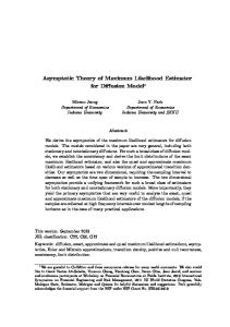
By substituting p(x; µ) to Iq and Jq , the variance of asymptotic normal distribution can be represented by ( ) Iq 3 (2 − q)3 for q < . (47) = Jq2 (3 − 2q)3/2 2 We plotted Eq. (47) (q < 3/2) in Fig. 1 (the solid line). As can been seen from this figure, q = 1 gives the minimum variance. This mean that q = 1 (MLE) is the most efficient for inference of µ. This is consistent with the fact that MLE of Gaussian mean is the efficient estimator, which attains the Cram´er-Rao bound. For the case of q ≥ 3/2, Iq is infinity, and the argument for the asymptotic Gaussian distribution can not be applied. We confirm Eq. (47) by computer simulation. We show histograms of MqLE for Gaussian mean at q = −1, 1 and 1.2 in Fig. 2. The number of samples used for inference of MqLE is N = 100000 and we repeated the inference 100000 times at each q. We also calculated the kurtosis of histograms. It is known that the kurtosis of Gaussian samples is 3. The kurtosis of q = −1, 1 and 1.2 are very close to 3. We can say from these results that the asymptotic distribution of Gaussian mean MqLE is the Gaussian distribution. As shown above, the variance of asymptotic Gaussian distribution of MqLE is represented by Eq. (47) for the case of q < 3/2. In Fig. 1, a solid line represents the analytical solution and circles describe the values obtained by the simulation. As can been seen from this figure, analytical results are in good agreement with computational one.

11

Figure 1: (Color online) Variance as a function of q calculated by analytic method (the solid curve) and simulation (circles).

Figure 2: Histogram of µ bq in Gaussian mean case for (a) q = −1, (b) q = 1 and (c) q = 1.2 (b µq is estimated with sample size of N = 100000, and this estimation is repeated 100000 trials). Distributions converge to the Gaussian distribution. We also show the kurtosis of each histogram. The kurtosis is 3 for the case of the Gaussian distribution.

12

Figure 3: (Color online) Effect of outliers on MqLE of Gaussian mean for (a) q ≤ 1 and (b) q ≥ 1. 3.1.3

Robustness

We calculated χq (xout ) for Gaussian mean. By using Gaussian distribution, we obtain the following equation: [ ] 1 q−1 (q−1) 2 (xout − µ) exp (xout − µ) . (48) χq (xout ) = (2π) 2 2 For q = 1, we get χq (xout ) → ∞ for xout → ∞: MqLE is greatly affected by an outlier. In contrast, for q < 1, we get χq (xout ) → 0 for xout → ∞: MqLE is robust against an outlier. For the case of q > 1, χq (xout ) → ∞ for xout → ∞. We plotted Eq. (48) for q = 0.0, 0.5, 0.9, 1.0 and 1.25 in Fig. 3. This figure shows that the effect of outliers can be tuned by changing q in MqLE. When q > 1, the effect of outliers are magnified and MqLE becomes more sensitive to outliers than the case of MLE (q = 1). We see the robustness properties by computer simulations. We generated samples from Gaussian distribution (µ = 0, σ 2 = 1), and added outliers at x = 10. We calculated MqLE of Gaussian mean with q = 0.0, 0.95, 1.0 and 1.25. Fig. 4 shows the result of this experiment. We can see from this figure that MqLE of q = 0 is not affected by outliers. On the other hand, q = 1 case is affected by outliers, and this can be confirmed by Eq. (48). Although the asymptotic variance of q = 0.95 is very close to q = 1, MqLE of q = 0.95 is much more robust than that of q = 1. This indicates that robustness of MqLE can be obtained almost without losing the efficiency of the estimator. As expected by Eq. (48), q = 1.25 is greatly affected by outliers.

3.2

q-Gaussian Distribution

In this section, we confirm the three properties of MqLE for the case of q-Gaussian distribution. q-Gaussian distribution is a generalization of the conventional Gaussian distribution. We let q˜ be an entropic index for q-Gaussian distribution and q for MqLE. q-Gaussian 13

Figure 4: (Color online) Robustness simulation in MqLE of Gaussian mean for q = 0, 0.95, 1.0 and 1.25. A histogram represents learning data and a rightmost bin is outliers. Lines describe estimated PDF in each q.

Figure 5: (Color online) q-Gaussian distribution (µq˜ = 0, σq2˜ = 1) for q˜ = −∞, 0, 1 and 2.

14

is derived from MaxEnt of Tsallis entropy under two constraints: ˆ µq˜ = x Pq˜(x)dx,

(49)

ˆ σq2˜

=

(x − µq˜)2 Pq˜(x)dx.

(50)

In these equations, µq˜ is q-mean, σq2˜ is q-variance and Pq˜(x) is the escort distribution ´ q˜ q˜ defined by Pq˜(x) := p(x) / p(x) dx. By carrying out MaxEnt principle to the Tsallis entropy under these constraints, PDF of q-Gaussian distribution is obtained by Eq. (51) (Fig. 5): { } 1 (x − µq˜)2 2 p(x; µq˜, σq˜) = expq˜ − , (51) Zq˜ (3 − q˜)σq2˜ where Zq˜ is a partition function represented by { } ˆ (x − µq˜)2 Zq˜ = expq˜ − dx (3 − q˜)σq2˜ √ ( )  3 − q˜ 2 1 1 1    σ B , − (for 1 < q˜ < 3)   q˜ − 1 q˜ 2 q˜ − 1 2  √ = 2πσq2˜ (for q˜ = 1)  √  ( )    1 1 3 − q˜ 2   (for q˜ < 1) .  1 − q˜σq˜B 2 , 1 − q˜ + 1

(52)

In Eq. (52), B(a, b) represents the beta function. For the case of q < 1, q-Gaussian has compact support and p(x; µq˜, σq2˜) is positive only on √ √ ( ) 3 − q˜ 2 3 − q˜ 2 µq˜ − σ , µq˜ + σ . 1 − q˜ q˜ 1 − q˜ q˜ The q-Gaussian given by Eqs. (51) and (52) reduce to the conventional Gaussian and Cauchy distributions for q˜ = 1 and q˜ = 2, respectively. 3.2.1

Consistency

In this section, we show the consistency of MqLE for q-Gaussian distribution. MqLE of q-Gaussian q-mean (1 < q˜ < 3) satisfies the nonnegativity condition when q ≤ 1. For the case of MqLE of Gaussian mean, the nonnegativity is also satisfied for q < 2 by direct calculation of Rajagopal divergence [Eq. (41)]. It is expected that MqLE for q-Gaussian q-mean also satisfies the nonnegativity condition for q > 1 region. However, we could not show the nonnegativity in this case analytically. We instead show the nonnegativity of Rajagopal’s divergence in a specific case that q = q˜ > 1 (entropic 15

index for MqLE and q-Gaussian are the same). Let p(x; µq ) := p(x; µq , σq2 = 1). DqRaj is calculated as follows for q = q˜:

DqRaj [p(X; µq˜,0 )||p(X; µq˜)]

(µq˜,0 − µq˜)2 qe−1 Zqe (for 1 ≤ q = qe < 5/3) = (3 − q˜) ≥ 0,

(53)

where µq˜,0 denotes a true parameter. We can see from Eq. (53) that DqRaj is nonnegative and DqRaj = 0 if and only if µq˜ = µq˜,0 . In Sec. 3.1.1, we have shown the inconsistency of MqLE ’s Gaussian variance. We followed similar consideration for MqLE of q-Gaussian q-mean. Let us consider the situation that q = q˜, and µq˜, σq2˜ are unknown. A parameter inference in this case is to estimate µq˜ and σq2˜. By considering the stationary points of q-log likelihood function, we obtain Eqs. (54) and (55): N 1 ∑ µq˜ = xi , N i=1 N ∑

3−q 2 σq˜ = 2

(54)

(xi − µq˜)2

i=1 N ∑

,

(55)

Uq˜(xi )

i=1

where Uq˜(x) := 1 −

(1 − q) (x − µq˜)2 . 2 (3 − q)σq˜

In the limit N → ∞, a similar consideration as the Gaussian case yields following relations: µq˜ → µq˜,0

(56)

3−q 2 2 σq˜ → σ2 . 2 5 − 3q q˜,0

(57)

We can see from these equations that only µq˜ is self-consistent, while MqLE of σq2˜ is not self-consistent except for q = 1. This indicates MqLE of q-variance is not a consistent estimator. 3.2.2

Asymptotic Distribution

We calculated the variance of asymptotic Gaussian distribution for p(x; µq˜). A lengthy calculation yields the following equation:

16

Figure 6: (Color online) Variance of asymptotic distribution for q˜ = 3/2 (the solid curve) and q˜ = 2 (the dashed curve) calculated by analytical method, circles denoting results of simulations.

Figure 7: Variance of asymptotic distribution (q-Gaussian mean with q = q˜) obtained by analytical (the solid curve) and computational methods (circles).

17

(

Iq Jq2

) ( ) ( )2 1 1 1 3 − 2q 2˜ q−q Γ + + Γ Γ 2 q˜ − 1 2 q˜ − 1 q˜ − 1 = q˜ ( ) ( ) ( )2 1 3 − 2q 1 2−q Γ 2+ Γ 2+ Γ + q˜ − 1 q˜ − 1 2 q˜ − 1 ) ( 5 1 for 1 < q˜ < 3, q < + q˜ 4 4

(58)

In this equation, q˜ is the entropic index of q-Gaussian, q is that of q-likelihood and Γ(x) is the gamma function. For the region of q ≥ 5/4 + q˜/4, Iq is infinity and the argument for the asymptotic Gaussian distribution can not be applied. For the case of q-Gaussian q-mean, q = 1 also attains the minimum variance. For q = 1, the variance is represented by Iq = q˜. Jq2 Cauchy distribution is covered by q-Gaussian distribution with q˜ = 2. Asymptotic variance of Cauchy location parameter can be obtained by substituting q˜ = 2 in Eq. (58): ( ) √ 7 ) πΓ − 2q Γ (4 − q)2 ( Iq 7 2 = for q < . (59) ( )2 Jq2 4 5 2Γ (5 − 2q) Γ −q 2 We plotted Eqs. (58) and (59) in Fig. 6. The shape of Fig. 6 totally resembles Fig. 1. As mentioned in the previous paragraph, MqLE of q-Gaussian q-mean, where q and q˜ is the same value, satisfies nonnegativity condition of Rajagopal’s divergence DqRaj [Eq. (53)] with 1 ≤ q < 5/3. Substituting q˜ = q in Eq. (58), the asymptotic variance for this case is represented by Eq. (60): ( ) Iq 3−q 5 = for 1 ≤ q < . (60) Jq2 5 − 3q 3 We plotted Eq. (60) (1 ≤ q < 5/3) in Fig. 7. As can been seen from this figure, q = 1 gives the minimum variance (MLE for the conventional Gaussian mean). Because this MqLE is simply obtained by averaging each xi , simply using the central limit theorem reaches to the same result. For the case of q ≥ 5/3, the asymptotic distribution is not Gaussian distribution. The sum of independent random variables, whose PDF having ∼ |X|−1−α (0 < α < 2) converges in distribution to the α-stable L´evy distribution. q2 Gaussian distribution behaves as ∼ |X| 1−q when |X| → ∞. Therefore MqLE converges in distribution to α-stable L´evy distribution (α = (q − 3)/(1 − q)).

18

Figure 8: Histogram of µbq˜q in q-Gaussian q-mean case for (a) q = −1.0, (b) q = 1.0 and (c) q = 1.25 (µbq˜q is estimated with sample size of N = 100000, and this estimation is repeated 100000 trials).

Figure 9: Histogram of µbq˜q in q-Gaussian q-mean case with q = q˜ for q = 1.1 and q = 1.9 (µbq˜q is estimated with sample size of N = 40000, and this estimation is repeated 100000 trials). For the cases of q = 1.1, distributions converges in distribution to Gaussian. On the other hand, when q = 1.9, asymptotic distributions are α-stable L´evy distribution.

19

We confirm the asymptotic Gaussianity and asymptotic variance by computer simulations. We first show histograms of MqLE for at q = −1, 1 and 1.25 in Fig. 8. We experimented with N = 100000 and 100000 iterations at each q. As can been seen with Fig. 8, each histogram is Gaussian distribution. Fig. 6 confirms the analytical calculations. In this figure, a solid and a dashed lines are the analytical solution for q˜ = 3/2 and 2, respectively, and circles are the computational solutions. We can see that computational results are well fitted to the analytical line. Although we can not show the nonnegativity for the case of q > 1 analytically, it seems that MqLE for q-Gaussian q-mean is a consistent estimator for this case. We have shown that the asymptotic distribution of MqLE q-mean is Gaussian for 1 ≤ q < 5/3 with q˜ = q. We calculated the variance of the asymptotic Gaussian distribution by computer simulation (N = 40000 with 100000 iterations). Obtained variances are shown in Fig. 7 where the solid line represents the analytical solution and circles describe the values obtained by the simulation. As can been seen in this figure, computational results agree with analytical calculations. Fig. 9 describes the histogram of asymptotic distributions. For q = 1.9, an asymptotic distribution of MqLE are not Gaussian and exhibits long tails, which is considered to be the α-stable L´evy distribution. 3.2.3

Robustness

We also calculated χq (xout ) for q-Gaussian distribution, as given by ) q−1 −1 q˜−1 q˜ − 1 2 (xout − µq˜) 1− 2(xout − µq˜) q˜ − 3 χq (xout ) = ·( ) 1−q ( )1−q . 3 − q˜ 2 1 1 1 2 ·B , − −1 + q˜ − 1 2 q˜ − 1 2 (

(61)

Fig. 10 describes the q˜ = 2 case of χq (xout ). For this case, MLE (q = 1 of MqLE) already satisfies χq (xout ) → 0 for xout → ∞. As a consequence, MLE of q-Gaussian qmean is already robust against outliers. χq (xout ) of q = q˜ case exhibits a linear relation. and MqLE of q = q˜ is neither robust nor efficient estimator. When q = (˜ q + 1)/2, χq (xout ) = O(1) for xout → ∞ and this is a marginal case between robust and nonrobust estimators: MqLEs of q ≤ (˜ q + 1)/2 and q > (˜ q + 1)/2 are robust and non-robust estimators, respectively. We experimentally confirm the robustness property of MqLE for q-Gaussian q-mean. Specifically, we used q˜ = 2 case (Cauchy distribution). We generated Cauchy random samples and add outliers to them. Fig. 11 describes the result of this experiment. In this figure, outliers are located at 5. We calculated MqLE of Cauchy location parameter with q˜ = 2 with q = 0, 1 and 2. For q = 2, a location parameter is the same as the sample mean (note that MqLE of this case is not a consistent estimator). For the case of MqLE of Gaussian mean (Sec. 3.1.3), q = 1 is not robust under outliers. On the other hand, from Fig. 11, MqLE (q = 1) of Cauchy location parameter is robust against 20

Figure 10: (Color online) Effect of outliers on MqLE of q-Gaussian q-mean (˜ q = 2: Cauchy distribution) for (a) q ≤ 1 and (b) q ≥ 1. In (b), q = 3/2 is the marginal case.

Figure 11: (Color online) Robustness simulation for MqLE of Cauchy location parameter with q˜ = 2 for q = 0, 1 and 2. Lines represent PDF estimated by MqLE of each q.

outliers. MqLE with q˜ = q = 2 is affected by outliers and this case is almost identical to MLE for Gaussian mean. These results indicate that MqLE is more effective to Gaussian mean than q-Gaussian q-mean, since MLE is already robust for q-Gaussian case.

4

Conclusion and Discussion

From analyses carried out in Sec. 2 and 3, the properties of MqLE under specific distributions are summarized as follows: • MqLE of Gaussian mean – For q < 3/2, asymptotic distributions are Gaussian. – q = 1 yields the smallest variance in the asymptotic Gaussian distribution. – For q < 1, MqLE with smaller q is more robust under outliers. 21

– For q ≥ 1, MqLE with larger q is more sensitive to outliers. • MqLE of q-Gaussian q-mean (1 < q˜ < 3, where q˜ is an entropic index of qGaussian) – For q < 5/4 + q˜/4, asymptotic distributions are Gaussian. – q = 1 yields the smallest variance in the asymptotic Gaussian distribution. – For q ≤ 1/2(˜ q + 1), MqLE with smaller q is more robust under outliers. – For q > 1/2(˜ q + 1), MqLE with larger q is more sensitive to outliers. Since there are many algorithms which are based on the Gaussian and q-Gaussian distributions, it is very interesting to apply MqLE to other applications. We have shown the asymptotic Gaussianity and the variance of the distribution analytically. Many statistical theories take advantage of the asymptotic Gaussianity of the estimator, and it may be important to expand these theories to MqLE. We limited the class of PDFs to Gaussian and q-Gaussian which satisfy the nonnegativity condition. It is of significance to investigate the sufficient condition for satisfying the nonnegativity condition for DqRaj . In Ref. [9], where the q-likelihood is proposed, the independence of random variables is not assumed. On the other hand, we assumed the independence in random variables. Under the independence assumption, MqLE is valid under a specific class of distributions. Recently, the concept of the independence has been generalized in nonextensive statistics [19, 20, 21]. Since conventional independent random variables are characterized by a product of the Fourier transform (the characteristic function), q-independence for example is defined by a q-product of a q-Fourier transform [19]. It is very interesting to see the relation between MqLE and the generalized independence in nonextensive statistics. We have denoted that MqLE is potentially applicable to location parameter. There are other distributions which satisfy this condition, such as logistic distribution, for example, which is represented by p(x; η) :=

1 exp (−(x − η)/β) (for − ∞ < x < ∞). β [1 + exp (−(x − η)/β)]2

It may be possible to apply MqLE to these kinds of distributions and this may be our future research topic.

References [1] C. Tsallis, Physica D 193 (2004) 1. [2] C. Tsallis, in: M. Gell-Mann and C. Tsallis (Ed.), Nonextensive Entropy, Oxford University Press, 2004, p.1. 22

[3] R. Stinchombe, in: M. Gell-Mann and C. Tsallis (Ed.), Nonextensive Entropy, Oxford University Press, 2004, p.139. [4] C. Beck, arXiv:cond-mat/050230v1, (2005). [5] C. Tsallis, J. of Stat. Phys. 52 (1988) 479. [6] E. T. Jaynes, Phys. Rev. 106 (1957) 620. [7] E. P. Borges, Physica A 340 (2004) 95. [8] L. Nivanen, A. L. M´ehaut´e, and Q. A. Wang, Rep. on Math. Phys. 52 (2003) 437. [9] H. Suyari, IEEE Trans. on Inf. Theory, 51 (2005) 753. [10] H. Suyari, Physica A 368 (2006) 63. [11] D. Ferrari, Center for Economic Research (RECent) 016, University of Modena and Reggio E., Dept. of Economics, May 2008. [12] C. Tsallis, Phys. Rev. E 58 (1998) 1442 [13] A. R´enyi, Proc. of the 4th Berkeley Symp. on Math., Stat. and Prob. (1960) 547. [14] A. K. Rajagopal, in: S. Abe and Y. Okamoto (Ed.), Nonextensive Statistical Mechanics and Its Applications, Springer, 2000, p.99. [15] O. H¨older, Nachr. Ges. Wiss. G¨ottingen (1889) 38. [16] A. Stuart, J. K. Ord, and S. Arnold, Classical Inference and the Linear Model, vol. 2A of Kendall’s Advanced Theory of Statistics, 6th Edition, Arnold, 1999. [17] L. Borland, A. R. Plastino, and C. Tsallis, J. Math. Phys. 39 (1998) 6490. [18] H. Shioya and T. Date, IEIC Tech. Rep. 100 618 (NC2000 93-102) (2001) 1. [19] S. Umarov, C. Tsallis, and S. Steinberg, arXiv:cond-mat/0603593v4 (2006). [20] L. G. Moyano, C. Tsallis, and M. Gell-Mann, Europhys. Lett. 73 (2006) 813. [21] A. Rodr´ıguez, V. Schw¨ammle, and C. Tsallis, arXiv:0804.1488v2 (2008).

23