Processes of Extinction James W. MINETT1, MA Hongbin2, Aurea M. PEREZ3, Qi Ji4, Adam B. SMITH5 WANG Yue6, YANG Hongfeng7, Aletta YÑIGUEZ8 1
Department of Electronic Engineering, Chinese University of Hong Kong, Sha Tin, Hong Kong, China. E-mail:
[email protected] 2Academy of Mathematics and Systems Science, Zhong Guan Cun East Road 55, Haidian District, Beijing 100080, China. E-mail:
[email protected] 3University of the Philippines, Baguio, Dept. of Mathematics and Computer Science, Gov. Pack Road, Baguio City 2600, Philippines. E-mail:
[email protected] 4The Institute of Theoretical Physics, Academia Sinica, 55# Zhong Guan Cun East Road, Beijing 100080, China. E-mail:
[email protected] 5Energy and Resources Group, 310 Barrows Hall, University of California, Berkeley, Berkeley, CA 94703-3050, USA. E-mail:
[email protected] 6Nanjing Institute of Geology and Palaeontology, Chinese Academy of Sciences, 39 East Beijing Road, Nanjing, Jiangsu 210008, China. E-mail:
[email protected] 7University of Science and Technology of China, Department of Earth and Space Sciences, Room 323-132, USTC, Hefei, Anhui 230026, China. E-mail:
[email protected] 8Marine Biology and Fisheries, Rosenthal School of Marine & Atmospheric Science, University of Miami, Key Biscayne, FL 33145, USA. E-mail:
[email protected]
Abstract To investigate the dynamics of extinction in a changing environment, we modified a model developed by Norberg et al. (2001, PNAS 98:11376-11381), in which species interact and grow in a logistic manner, but their performance is modified by the distance between their phenotypes and the environment. We found that both the original and modified model were very sensitive to the ratio between mortality and growth, with extinction rates and their qualitative form often decided by the ratio between the two. By increasing environmental amplitude, we were able to generate “stepwise” extinction events similar to those in past mass extinctions composed of alternating periods of high then low extinction rates. We also found extinction rates increase as the magnitudes of step disturbances and linear trends in the environment rise. In light of the diversity-stability debate in ecology, we found little effect of initial species richness on the qualitative behavior of the system, including persistence and extinction rates, the one exception being that more diverse systems have a lower probability of total extinction after an arbitrary percentage of species are removed. We also note possibilities of extension of the model into other fields, such as using it to predict phonetic change in language. Introduction Our world faces a major biological and cultural extinction crisis: 90% of all languages will likely be moribund or lost by 2100, and 25% of the world’s species will probably be “on the road to extinction” by 2050 (Krauss 1992, Thomas et al. 2004). Understanding the dynamics of diversity loss, as well as the consequences of losing diversity, is critical not only in preventing extinctions, but also determining the effect such unprecedented eradications have on the functioning of societies and ecosystems. To explore the dynamics of extinction, we modified a model originally developed by Norberg et al. (2001) who examined the effect of a changing environment on a suite of competing species that differ in their fitness to the environment. We chose this model because it is general and based on functional forms many ecologists use today but are nevertheless venerable (for example, it utilizes the logistic growth equation used by Lotka and Volterra in the 1920’s to model competition). Here we report results of our extensions to the model, including allowing exploitation and facilitation (not just competition), catastrophic extinctions, and species
invasions. We also examine different environmental forcing functions like gradual, step, and random changes. Throughout, we also report on model sensitivity and note model weaknesses. Finally, though the model is originally intended to represent ecological systems, we also discuss a possible extension to the field of linguistics. Methods We extended the basic model developed by Norberg et al. (2001) which portrays Bj,t, the dynamics of biomass of species j at time t with a modified logistic growth equation: B j ,t +1 = B j ,t + B j , t ⋅ p ⋅ X (P, E ) ⋅ (1 − A(K , α , B )) − B j , t ⋅ d
Equation 1
in which p and d are respectively fertility and death. X(Pj, Et) is the environmental forcing function, which modifies species j’s growth:
(
X (P, E ) = exp − (Et − Pj )
2
)
Equation 2
in which species j has a phenotype Pj which, relative to the current state of the environment Et, determines its performance as expressed by the exponential term in the equation. A(K, , B) is the interaction function, which modifies the growth of species j according to the effect other species have on the growth of species j and the effect species j has on itself, A(K , α , B ) =
1 K
N k =1
α jk Bk , t
Equation 3
Here, K is carrying capacity of the environment, N is the number of species in the community, and jk is the per-unit biomass effect species k has on j. When j = k, jk was always set to −1 (referred to below as “full competition”). Norberg et al. explored cases in which all species competed against each other perfectly (all jk = −1), which we used as our default setting for exploring scenarios. We also examined cases in which jk = 0 for all j k (referred to as “intraspecific competition”). The original model also includes the addition of an immigration term i, but in all of our analyses we set this term = 0. In order for a species to go extinct in the modified model, we set an arbitrary cutoff of 0.01·K, meaning that if the biomass of a species achieved 1% of carrying capacity, it went extinct. Unless otherwise stated below, we used standard parameter values to explore various scenarios. Phenotype was constrained and evenly distributed among species between 0 and 1. Fertility p and death d were each set to 0.1, and carrying capacity K to 10. Each species began with a biomass Bj,0 of N/K. Typically we used an environmental function for E which generated a sinusoidal curve with an amplitude of 0.3, a mean of 0.5, and a period of 100 time units. We also explored the effects of adding uncorrelated noise, linear increases, step functions, and adding a longer-period sine wave to the environmental function in order to depict certain scenarios relevant to extinction dynamics (see below for details). Finally, we examined scenarios in which the community experienced random invasions by new species and random extinctions of extant species over time.
Effect of increasing environmental period In this experiment, we examine the patterns of extinction of species as a function of the period of a sinusoidally varying environment. The sinusoidal periods we examined were of 400, 1200 and 2000 time steps; in each case, the experiment was run for a total of 10,000 time steps of an environment having amplitude 0.6. Figure 1 shows the resultant plots for the trajectories of both total biomass and the cumulative number of extinct species. Examining first the biomass plots, we observe that the biomass oscillates with a period half that of the corresponding environment. For each value of the environmental period, the total biomass reaches a maximum each cycle of about 2.5, about one quarter of the notional carrying capacity, 10. However, the local minima of the biomass alternate between a relatively slight drop from the maximum value at one local minimum to a substantial drop at the next local minimum, a phenomenon that becomes more pronounced as the environmental period is increased. This can be explained by considering the fitness of a species with phenotype 0.9: In our implementation of the modified Norberg model, the fitness of a species is defined in terms of its phenotypic value Pj and the state of the environment Et by (Equation 2: X = exp[−(Et − Pj)2]). Observe that the fitness is maximal when Et equals Pj, which occurs twice per environmental cycle. Similarly, the fitness achieves a local minimum twice per cycle, once when the state of the environment is maximal and once when it is minimal, but note that the fitness is least when the environment reaches its minimal state. The biomass of each species therefore cycles with a period half that of the environment. Notice too that as the environmental period is increased, so the length of time during which a species is unfit is increased, so increasing the likelihood that the species becomes extinct, thereby causing greater fluctuation in the total biomass. Examining now the extinction plots, we observe that long-period environments lead to greater rates of extinction; this is due to the increased duration in which each species is unfit. Furthermore, it is evident that as the period is increased, so the mode of extinction gradually shifts from gradual extinction to increasingly stepwise extinction, the epochs of mass extinction coinciding with the global minima of the total biomass. Eventually, if the period and amplitude of the environmental state are sufficiently great, the entire system will become extinct in a single catastrophic extinction event. Effect of increasing relative mortality We now consider the role of the fertility rate, p, and mortality rate, d, on the extinction pattern. For convenience, we only present results where all species have the same fertility and mortality rates. The environment period was set to 1,000 time steps and the amplitude to 0.6. In each run, the fertility, p, was set to a value on the interval [0.1, 0.2] and the mortality, d, was set to some fraction of the fertility; the resultant measure of “relative mortality,” d / p, was allowed to vary on the interval [0.5, 1.0]. For each run, the number of extinction events before the entire system became extinct were counted – extinction of the entire system in a single event corresponds to catastrophic mass extinction, while extinction in many events corresponds to gradual mass extinction. Figure 2 shows a contour plot of the number of extinction events before total extinction occurred for different values of the fertility and relative mortality. The figure suggests that relative mortality has a more significant effect on the extinction pattern than fertility, with high relative mortality — >0.75 for the scenarios examined — leading to catastrophic mass extinction, and lower values of relative mortality leading to progressively more gradual mass
extinction. For a fixed value of the relative mortality, however, a greater value of the fertility (and hence also the mortality) pushes the system toward catastrophic mass extinction. One modest conclusion that we can draw from this experiment is that relatively stable ecosystems in which species have relative mortality close to the value 1 are at significant risk of catastrophic extinction should the fitness of species be negatively impacted by environmental change. It would be instructive to examine also the role of heterogeneity in the value of relative mortality.
Does diversity matter? Invasive species and extinctions The number of species in an ecosystem or the whole biosphere is not static. There are two ways of looking at the dynamic nature of diversity in biological systems. One is through an evolutionary perspective wherein new species evolve. Another is at an ecological level, where new species come into new habitats from other areas. The ecological perspective can be seen as an “invasive species” problem wherein new species are introduced into areas where they were not normally found. The introduction of exotic species has been pinpointed as one of the threats to current biodiversity and extinction of native species (Novacek and Cleland 2001). For example, 200 endemic cichlids became extinct after the Nile Perch was introduced in Lake Victoria (Witte et al. 1992). However, not all introductions lead to extinctions of native species. This has led to questions regarding a system’s “invasability.” What makes a system vulnerable to the establishment and domination of invasive species? One hypothesis states that the species richness of a system plays a role in the effect of species invasion events (Elton 1958, Lodge 1993). This hypothesis was investigated with the extended Norberg et al. model by introducing a certain percentage of new phenotypes or species at the 50th time step in systems with different species richness. Simulations were run with different number of species (5, 10, 20, 30, 40, and 50) and different percentages of introduced new species (1, 5 and 10%) relative to the initial number of species as well as two different competition levels (full interspecific where all jk = −1 and only intraspecific competition where jk = 0 but jj = −1). No catastrophic extinction was observed for any of the scenarios explored, even if the system was species-rich or species-poor. There was some quantitative difference, wherein as you increase the number of species in the system, there was also a slight increase in the mean percentage of extinction. There was also a quantitative difference between the base model run (no invasion) and the 10% species invasion in a system with 50 “native” species (85% vs. 98% mean extinction, respectively). This relationship was seen more strongly in simulations where there was full interspecific competition. This highlights the strong influence of interaction effects. The more species are competing, the more extinctions occur. These results seem to say that the more diverse a system is, the more extinctions you see as these are invaded. This contradicts the hypothesis that diversity serves as a buffer to invasability. This contradiction may be due to structure of the model itself, where all species compete negatively, between and/or within species, and does not allow for other interactions (positive and neutral) observed in ecosystems. Unfortunately as well, there is no way to know which species survived until the end of the model run, which would be a more concrete test of the system invasability. Effect of increasing species interaction We now examine the effect of different degrees of species interaction on the observed patterns of extinction. In addition to the default case of “full competition” in which the inter-species
competition is set to be equal to the intra-species competition (i.e., ajk = –1 for all j, k), we also examine the effect of “partial competition” (ajj = –1 for all j; ajk = –½ for all j k), “random competition” (ajj = –1 for all j; ajk uniformly distributed on [–1, 0] for all j k), and “random competition with exploitation” (ajj = –1 for all j; ajk uniformly distributed on [–1, +½] for all j k). In the latter scenario, we model both competition, characterized by a negative value of ajk for both species j and k, and exploitation, characterized by a positive value of ajk for the exploiting species (e.g., a predator) and a negative value of ajk for the exploited species (e.g., its prey). In each case, the simulation was run for an environment with period 1,000 and amplitude 0.3; the fertility was set to 0.1 and the mortality to 0.05. Figure 3 shows the results of the experiment. It is evident that the “full competition” scenario, in which each organism competes equally with each organism, supports the least biomass. The “partial competition” scenario supports only slightly more biomass, but results in fewer species going extinct: about 70% for “partial competition” versus about 80% for “full competition”. This phenomenon results because, for “partial competition”, species that are unfit with respect to the environment undergo less inter-species competition than in the “full competition” scenario, so maintaining greater biomass and greater species diversity. When diversity in the interaction weights is introduced in the “random competition” scenario, modeling more realistically the heterogeneous interactions expected in an actual ecosystem, changes in biomass of different species affect each other in different ways – if a species with low interaction weight with respect to another particular species increases in biomass, it will have little impact on the second species; however, if the interaction weight is close to –1, its own biomass may fall significantly due to the competition. The increased heterogeneity in the competition reduces the number of “niches” available in which species can survive, so leading to a greater number of extinctions. The expected value of inter-species competition remains –½, as for “partial competition”, so the total biomass is approximately equal. The “random competition with exploitation” scenario supports the fewest species yet, somewhat paradoxically, attains the greatest biomass. This arises because some species are able to exploit others, thereby increasing in biomass as the biomass of the other species grows. The potential increase in total biomass is tempered, however, by the risk that as the biomass of such an exploiter increases dramatically, causing other species with which it does compete to go extinct. This scenario appears to reach a stable state far quicker than the other scenarios, after which extinction “switches off”. This results suggests that an ecosystem comprising species having a diversity of phenotypes and interactions is stable once the initial period of competition-driven mass extinction is passed without total collapse of the ecosystem.
What happens after a mass extinction? Effects of arbitrary extinction events and diversity Another aspect that was investigated using the extended Norberg et al. model was the question of resilience and recovery of systems after different intensities of extinction events. In ecological systems, the extinction of species can disrupt and shift them towards a different community structure. For example, local extinctions of the sea otter Enhydra lutris in western Alaska led to local extinctions as well of the kelp forests due to the high abundance of its grazer (Estes et al. 1998). Can such shifts be avoided if the systems were species-rich? Does diversity serve as a buffer to the extinction of the system? Species diversity in ecosystems is believed to contribute to ecosystem function through mechanisms such as enlarging the range of species traits and the concomitant increased pathways of resources within the system (Nijs and Impens 2000). Higher species diversity can also lead to functionally redundant species (Naeem 1998). The loss of
ecosystem function could potentially lead to more extinction. To investigate the effect of diversity and interactions on extinction events, simulations were run using different numbers (5, 10, 30, 40, 50) of species and competition intensities (full interspecific and only intraspecific competition). At the 50th time step, 10, 50 and 90% of the species in the system were arbitrarily made to go extinct. These simulations showed that higher number of species served as a buffer from extinction (Figure 4). The more species there are, the less the system slides into total extinction and more species are likely to survive (Figure 4b). The number of species needed to buffer a system from total extinction depends on the intensity of the initial extinction event. Figure 4a shows the total extinction of a system with only 10 species that underwent 90% extinction, however, the simulation with the same number of species but only experiencing 50% extinction was able to avoid total extinction (Figure 4c). The relation between species diversity and extinctions is mediated by the functioning and interactions of the species (Petchey 2000). Unfortunately, the extended Norberg et al. model does not take species function into account. Differentiation of these functions needs to be incorporated in order to tease out the finer points of the relationship between biodiversity and extinctions.
Does diversity matter? Diversity vs. stability The role of species diversity in determining stability of an ecosystem has been hotly debated for over a century. Since Steven Forbes 1887 argued that complex communities yield stability, ecologists presumed that complex systems were stable. More recently, theoretical (May 1972, Ives et al. 1999) and empirical (Tilman and Downing 1994, Tilman et al. 1994, Tilman 1996) studies have indicated that complex systems may not be stable in the sense that population dynamics of individual species fluctuate more in diverse systems. These same studies show that gross measures of the community, such as total biomass, are nevertheless more stable in diverse settings. We examined the effect of diversity on community persistence by running a default scenario (parameter values noted above) and varying only N from 10 to 20 to 50 to 100 species. We examined the effects of a different environmental mean, environmental amplitude, linear increase in environment (e.g., “global warming”), environmental noise with cycling, noise with no cycling, and a step disturbance (Figure 5). The intent was to discover the effect of diversity on the overall persistence of the community under different environments. As depicted in Figure 6, species richness did not affect the qualitative rate of species loss and each level of richness barely had a quantitative effect on the rate of extinction. The most dramatic effect was evoked by a reduction in amplitude of environmental cycling – both noise without cycling (Figure 6d) and a lower amplitude (Figure 6e) displayed slower rate of extinction compared to the other simulations, and had total community extinction not before time step 1700 . The remainder experienced total community extinction by time step 650, with little variation both between environments and levels of diversity. Total community biomass trends displayed similar patterns (not shown), indicating that ecosystem processes such as C-sequestration would be insensitive to species richness. Our model is based on one of the most commonly-used models in ecology, the LotkaVolterra logistic competition. Nevertheless, we demonstrate no effect of species diversity on the stability of communities in a variety of environments. This contrasts with theoretical and empirical findings by others (Kinzig et al. 2002).
Simulating past mass extinctions Since the recognition of extinction by the great French paleontologist Georges Curvier in the early 19th century, the subject was largely ignored until early in the 20th century, when a series of papers focused on the end-Permian mass extinction were published (Schindewolf 1954; Newell 1962). Raup and Sepkoski (1982) made the first statistical analysis of extinction rates at the family level, and confirmed the five major episodes with abrupt decreases in diversity, which have been accepted as the ‘big five’. Intensive studies on the patterns and mechanics of the mass extinctions have been made since then, especially of the end-Cretaceous and end-Permian events. However, the definition of the term ‘mass extinction’ is designed to be somewhat vague in that a mass extinction is an extinction of a significant proportion of the world’s biota in a geologically insignificant period of time (Hallam and Wignall 1997). It is interesting to notice that the Norberg model, to a certain extent, provides an interactive way to describe the changes of the environment and its corresponding extinction rate. As has been discussed above, the diversity of the species takes few effects on the rate of extinction. The following tests will only focus on the change of the environments. Three tests regarding to the abrupt, linear and cycling changes of the environments have been applied using the Norberg model. First, for the abrupt changes, the extinction rate increases in accordance with the change in mean amplitude of the environments (Figure 7). It shows a pattern of gradual extinction when the change in mean amplitude of the environment is less. When the amplitude is large enough, there will be an abrupt extinction, showing a greater extinction rate. This test demonstrates the process of the extinction pattern changing from gradual to sudden. However, the definition of gradual and sudden extinction is artificial. The test for the linear environmental changes then has the same results: with the increasing of the slope of the linear equation (Figure 8), the extinction rate increases, the pattern of extinction changes from gradual to sudden. Lastly, the cycling environmental change was applied, and results in a different pattern of extinction – the stepwise extinction. As showing in Figure 9, the steps depend on the amplitude of the changing environment as well as the duration of each period. Weaknesses of the model From the simulation results shown above, we can see that traditional equilibrium-type analysis can not be applied to the model by Norberg et al., which shows phenotypic diversity related with the global environment and external inputs. This simple model behaves in a somewhat complex manner though it looks simple. The model does suffer from some limitations, however. First, it weighs the environment too heavily; the environment is the main factor that influences the change of biomass. We consider it the essential defect of this model. This can be seen from the form of the function that affects the environment, exp[−(Et − Pj)2] from Equation 2. When biomass is far from the global environment, this term is very small (almost vanished), so only the so-called “mortality” d plays an important role. Second, the external inputs introduced in this model are necessary for overall persistence, but too arbitrary. To model the phenotypic diversity, it is natural to consider the external factors, however, it is considerable whether they are introduced like Norberg et al.’s model. In fact, the global environment is also a part of external factors, and Norberg et al. introduce the so-called external inputs to try to model the local fluctuation of each biomass. However, this approach is quite difficult to implement in practice because these terms are not easy to quantify; and the
arbitrariness of external input term i makes the model can behave like anything you want in mathematics. Norberg et al don’t make assumptions on external inputs yet, so mathematical analysis for this model is not possible in general. Third, maximum biomass would not normally remain as a constant, which may restrict the applications of this model, because in some cases the total biomass would change with the environment. Fourth, the number of phenotypes is a constant in this model, which may also restrict the applications of this model. No new phenotypes can be generated. So this model may not be proper for modeling the extinction and evolution, and essential mechanics of this model may not model mass extinction well. Finally, the model possesses too many parameters. A good model should be applicable, powerful, maybe beautiful, yet with parameters as few as possible. Too many parameters, some of which are even arbitrary, will restrict the applications of this model. A good model should reflect reality, but can be an abstraction or approximation of reality, and we needn’t use many parameters to fit reality as closely as we can. Even if we can tune the parameters to fit the present or training data well, such a model may have poor generality for future data. We also note that in the original presentation of the model, Norberg et al. present an environment generated with random noise, the so-called “reddened noise”, which may not be mathematically proper. This model is given in form of differential equations, not difference equations, and thus to guarantee the existence and continuousness of the solution of this model we can’t introduce a noise term arbitrarily.
Potential application to linguistics: Modeling diffusion of a sound change The Norberg model was devised specifically to model phenotypic diversity of species interacting in an ecosystem in response to changes in environment. Nevertheless, the model might also be applicable to other domains in which entities compete for resources in response to some “environmental” driving force. As a first step in such a direction, we consider briefly its potential application to modeling the diffusion of a sound change. Sound changes occur frequently, often making languages from times past almost incomprehensible to us if they were spoken to us now. The Great Vowel Shift, which was ongoing in English from the fifteenth century until the eighteenth century, resulted in the entire vowel system shifting from the Middle English (ME) system to the system that we now have in Modern English (ModE). The process of raising resulted in the first formant frequency of most vowels increasing, so that ME /ge:s/ came to be pronounced /gi:s/ ‘geese’ in ModE, while ME /go:s/ became ModE /gu:s/ ‘goose’. As the sound change became established, more and more speakers would have chosen to use the novel raised form instead of the original ME form. At some point, the raised form for a particular vowel would have been considered the standard form, at least in certain social and contexts, and so pressure would have been applied on speakers to adopt that form. This situation is rather similar to the role of environment in determining the fitness of a species having a particular phenotype, and suggests that the Norberg model might be applied to the modeling of the diffusion of a sound change. As a preliminary experiment, we translate the Norberg model to deal with a hypothetical sound change in the following: we assume that two sounds (phonemes) that differ only in terms of their first formant frequency compete for speakers in some population. The formant frequencies replace the phenotype in the Norberg model, varying on the normalized range [0, 1]; thus each phoneme may have a variety of pronunciations (phones) that are used by different
speakers. The number of speakers of each phone replaces the biomass in the Norberg model. The environmental state is replaced by the formant frequency of the form that the community prescribes to be the standard form, thereby imposing pressure on speakers to adopt that form. In particular, we examine how a change in the prescribed standard form results in the diffusion of a sound change across the population. Figure 10 shows the results of this experiment. The initial form, with formant frequency 0.25, is labeled f1 and the later form, with formant frequency 0.75, is labeled f2. The community prescribes f2 as the standard form from time step 1,000 onwards. What does the Norberg model predict will happen? Prior to f2 becoming prescribed, f2 phones (having formant frequency exceeding 0.5) are discarded, resulting in the standardization of f1. However, once f2 becomes prescribed, f1 phones are quickly lost, resulting in a rapid shift in the mean formant frequency towards that of f2. By this time, however, all forms with high frequency have already been lost, resulting in the majority of speakers adopting a form with intermediate formant frequency, 0.5. The resultant behavior is therefore a gradual diffusion of the intermediate form across the population. The model is, of course, highly simplistic, ignoring many of the subtleties that arise in a sound change. For example, the Norberg model allows the total number of speakers (biomass) to vary freely. However, in a situation of sound change, it is exceedingly unlikely that the change would cause the total number of speakers to change, just the numbers of speakers using the various competing forms. If an extension of the Norberg model were to be contemplated for application to modeling sound change, the model would have to be constrained to hold the total number of speakers (biomass), or to allow it to be specified as a function of time. Although the preliminary experiment reported here is intriguing, clearly much work will have to be done before the Norberg model can used to investigate substantively the diffusion of sound change, or, for that matter, other phenomena outside the realm of phenotypic diversity in ecosystems.
Conclusion Our investigations of a modified version of the model presented by Norberg et al. (2001) cover the sensitivity of the model to both its original parameters and also our modifications. In particular, we note the sensitivity of the model to the ratio of mortality to fertility, d / p, or “relative mortality,” a point not discussed by Norberg et al. When this ratio is high, the system tends toward catastrophic extinction, but even for a fixed value of relative mortality, as the values of fertility and mortality increase, the system tends toward the same disastrous end. We also found that diversity equivocally affects system stability and persistence. Modifications to which we found no qualitative difference in responses of the system included invasions, change in mean environment, addition of environmental noise, linear trends in the environment, step disturbances, and changes in environmental amplitude. In contrast, we did find that increasing the number of species in a system did decrease the risk of complete extinction after arbitrary extinction events wiped out a predetermined percentage of species. Norberg et al. used a “full competition” scenario for their initial investigations, in which each species impacted itself and others equivalently. Reducing competition increased overall community biomass, but ironically also increased the extinction rate, because species good at exploiting others disproportionably increased in biomass but at the same time were more vulnerable to demise after exploitees went extinct. We also note that the particular environmental forcing applied to the system determined qualitatively the rate and form of the extinction events. Not surprisingly, increasing the
magnitude of step disturbances, linear trends, and environmental amplitude increases the extinction rate, but larger amplitudes result in stepwise extinctions where alternating periods of high and low extinction rates followed one another. The model Norberg et al. developed and our modified version suffer from the “modeler’s curse” – they are both inflexible on some accounts and not complex on others. We do note that even the original model has a great number of variables which require an extensive sensitivity analysis to which we have hopefully contributed. However, we do suggest that with modification, the Norberg model might be extended beyond the field of ecology into other demesnes where extinction is also a pressing problem.
Biomass
0
10
10–2
0
1000
2000
3000
4000
5000
6000
7000
8000
9000
10000
Extinctions
100 80 60
Period 400 Period 1200 Period 2000
40 20 0
0
1000
2000
3000
4000
5000
6000
7000
8000
9000
10000
Time
Figure 1 Effects of environmental oscillation period on total biomass and number of species going extinct. Each simulation began with N = 100 species.
1 0.95
Relative Mortality, d / p
0.9 0.85
Catastrophic Extinction
0.8 0.75 0.7 0.65 0.6 0.55 0.5 0.1
Gradual Extinction 0.11
0.12
0.13
0.14
0.15
0.16
0.17
0.18
0.19
0.2
Fertility, p
Figure 2 Effects of fertility and “relative mortality” (= mortality rate / fertility rate = d / p) on the pattern of extinction.
Biomass 102
100
10–2
0
1000
2000
3000
4000
5000
6000
7000
8000
9000
10000
Extinctions
100 80 60
Full Partial
40 20 0
0
1000
2000
3000
4000
5000
Time
6000
7000
Random Exploitation 8000
9000
10000
Figure 3 Effects of different degrees of inter-species interaction on total biomass and number of species going extinct. In each scenario jk = −1 for all j = k, but for all j k, jk = −½ (“partial competition”), or was randomly distributed on the range [−1, 0] (“random competition”) or [−1, ½] (“random competition with exploitation”). Each simulation began with 100 species.
ENVIRONMENT
a 1
0.5
0
0
500
1000
1500
2000
2500
3000
3500
4000
4500
5000
3000
3500
4000
4500
5000
3000
3500
4000
4500
5000
3000
3500
4000
4500
5000
b
10
5
SPECIES EXTINCT
0
0
500
1000
1500
2000
2500
c
100
50
0
0
500
1000
1500
2000
2500
d
10
5
0
0
500
1000
1500
2000
2500
TIME
Figure 4 Results from simulations looking at recovery of systems with a default environment depicted in (a) from an arbitrarily imposed (b) 90% extinction rate with 10 species; (c) 90% extinction rate with 100 species; and, (d) 50% rate extinction with 10 species. Extinction events were imposed at the 50th time step.
a
1.50 Standard Scenario Lower Mean Lower Amplitude Linear Increase Step Disturbance
1.25 1.00 0.75 0.50
ENVIRONMENT
0.25 0.00 0
200
400
600
800
1000
b
1.00
0.75
0.50
0.25 Noise with Cycling Noise without Cycling
0.00 0
200
400
600
800
1000
TIME
Figure 5 Environments under which the effects of variation in diversity was tested as depicted in Figure 6. The environments were simulated up to 1000 time steps for illustration in the figure, but were continued to 2500 time steps for the actual simulations. a. Deterministic environments. The standard scenario used the default values stated in the text. Other differed from the standard scenario in that they had a different mean (“Different Mean” series, 0.3), amplitude (“Amplitude” series, 0.1), increasing linear trend (“Linear Trend” series, 0.001/time step), and a step disturbance (“Step Disturbance” series, addition of 0.2 at time step 300). b. Noisy environments. The series “Noise with Cycling” is the standard scenario plus an evenlydistributed random variable ∈ [−0.15, 0.15]. The series “Noise without Cycling” is the same except without a sine wave.
Environmental Mean: Proportion
Standard: Proportion Extinct
a
1.0
b
1.0
0.8
0.8
0.6
0.6
0.4
0.4
0.2
0.2
standard scenario
lower environmental mean
0.0
0.0 0
500
Environmental Noise: 1000 1500Proportion 2000
PROPORTION EXTINCT
2500
c
1.0
0
Environmental Cycling: Proportion 500 1000Noise sans 1500 2000
0.8
0.8
0.6
0.6
0.4
0.4
0.2
2500
d
1.0
0.2
noise with cycling
noise without cycling
0.0
0.0 0
= 0.10: Proportion 500Environmental 1000 Amplitude 1500 2000
2500
e
1.0
0
500
Global Proportion 2000 1000 Warming: 1500
1.0
0.8
0.8
0.6
0.6
0.4
0.4
0.2
0.2
2500
f
lower amplitude
linear increase
0.0
0.0 0
500
1000
1500
2000
2500
0
Environmental Proportion 500 1000 Step Disturbance: 1500 2000
g
1.0
2500
0.8
N = 10 N = 20 N = 50 N = 100
0.6
0.4
0.2
step disturbance 0.0
TIME
0
500
1000
1500
2000
2500
Figure 6 Effects of diversity on proportion of species going extinct under differing environments depicted in Figure 5. a. Standard scenario (default parameter values as in Methods; all following scenarios use the same parameter values except as noted). b. Lower environmental mean c. Environmental noise with cycling d. Environmental noise without cycling e. Lower environmental amplitude f. Linear environmental increase g. Step disturbance.
ENVIRONMENT EXTINCTIONS ENVIRONMENT EXTINCTIONS ENVIRONMENT EXTINCTIONS
a
1 0.5 0 100 50 00
500
1000
1500
2000
2500
1500
2000
2500
b 1 0.5 0 100 50 0 0
500
1000
c
1 0.5 0 100 50 0
0
500
1000
1500
2000
2500
TIME
Figure 7 Species extinction rate under different stepped environmental changes. a. No step change (mean environment = 0.2), extinction rate = 5%; b. Step change from a mean environment of 0.2 to 0.6, extinction rate = 6.7%; c. Step change from a mean environment of 0.2 to 1.0, extinction rate =38.7%.
0.5
100
1
EXTINCTIONS
ENVIRONMENT
EXTINCTIONS
EXTINCTIONS
00
ENVIRONMENT
ENVIRONMENT
a 1
500
1000
1500
2000
2500
500
1000
1500
2000
2500
50 00
b 0.5 00
500
1000
1500
2000
500
1000
1500
2000
2500
2500
100 50 00
c 1 0.5 00
500
1000
1500
2000
2500
500
1000
1500
2000
2500
100 50 00
TIME
Figure 8 Species extinction rate under different linear environmental changes. a. Linear rate of change = 0.00001/time step, extinction rate = 4.9%; b. Linear equation rate of change = 0.0001/time step, extinction rate = 5.6%; c. Linear rate of change = 0.01/time step, extinction rate =70%.
ENVIRONMENT EXTINCTIONS ENVIRONMENT EXTINCTIONS
a
1
b
1 0.5
0.5 0 0
500
1000
1500
2000
0 2500 0
100
100
50
50
0 0
500
1000
1500
2000
2500
500
1000
1500
2000
2500
1000
1500
2000
2500
3 2
0 0
1 500
c
1
d
1 0.5
0.5 0 0
500
1000
1500
2000
0 2500 0
500
100
100
2
50
50
1
0 0
500
1000
1500
2000
2500
1000
1500
2000
2500
2 1
0 0
500
1000
1500
2000
2500
TIME
Figure 9 Species extinction rate under different cycling environmental changes. a. Environmental amplitude = 0.2, environmental period = 400, extinction rate over time of extinction = 5.0%; b. Environmental amplitude = 0.4, environmental period = 500, extinction rate for steps 1, 2, 3 = 28%, 28.4%, 35.2%; c. Environmental amplitude = 0.4, environmental period = 800, extinction rate for steps 1, 2 = 18.2%, 40.8%; d. Environmental amplitude = 0.8, environmental period = 800, extinction rate for steps 1, 2 = 36.6%, 55%. Mean Normalized Frequency, F1
1
f2
0.8
f1
0.4
f2 adopted as standard form
0.6
0.2 0
0
1000
2000
3000
4000
5000
6000
7000
8000
9000
10000
8000
9000
10000
Normalized Frequency of Phones Discarded, F1
1 0.8 0.6 0.4 0.2 0
0
1000
2000
3000
4000
5000
Time
6000
7000
Figure 10 Diffusion of a sound change after a change in the prescribed standard form.
Acknowledgements We would like to thank Santa Fe Institute for its generosity in organizing and supporting Complex Systems Summer School. We also appreciated encouraging discussions with Doug Erwin and John Holland. Literature Cited Elton, C.S. 1958. The Ecology of Invasions by Animals and Plants. Methuen, London, UK. Estes, J.A., Tinker, M.T., Williams, T.M. and Doak, D.F. 1998. Killer whale predation on sea otters linking oceanic and nearshore ecosystems. Science 282 (5388) 473-476. Forbes, S.A. 1887. The lake as microcosm. Bulletin of the Peoria Scientific Association, pp. 77-87. Reprinted in the Bulletin of the Illinois State Natural History Survey 15(1925):537550. Reprinted in L.A. Real and J.H. Brown (eds.) Foundations of Ecology, Classic Papers with Commentaries. (1991) pp. 14-27. Hallam, A. and Wignall, P.B., 1997. Mass Extinctions and Their Aftermath. Oxford University Press. 320 pp. Ives, A. R., K. Gross, and J. L. Klug. 1999. Stability and variability in competitive communities. Science 286:542-544. Kinzig, A.P., Pacala, S.W., and Tilman, D. (eds.) 2002. The Functional Consequences of Biodiversity. Princeton University Press, Princeton, NJ. 366 pp. Krauss, M. 1992. The world' s languages in crisis. Language 68:6-10. Lodge, D.M. 1993. Species invasions and deletions: community effects and responses to climate and habitat change. In: P.M. Kareiva, J.G. Kingsolver, and R.B. Huey (eds.), Biotic Interactions and Global Change. Sinauer, Sunderland, Massachusetts, USA. May, R. M. 1972. Will a large complex system be stable? Nature 238:413-414. Naeem, S. 1998. Species redundancy and ecosystem reliability. Conservation Biology 12: 3945. Newell, N.D., 1962. Paleontological gaps and geochronology. Journal of Paleontology 36:592610. Nijs, I. and Impens, I. 2000. Biological diversity and probability of local extinction of ecosystems. Functional Ecology 14(1): 46-54. Norberg, J., D. P. Swaney, J. Dushoff, J. Lin, R. Casagrandi, and S. A. Levin. 2001. Phenotypic diversity and ecosystem functioning in changing environments: A theoretical framework. Proceedings of the National Academy of Sciences of the United States of America 98:1137611381. Novacek, M.J. and Cleland, E.E. 2001. The current biodiversity extinction event: scenarios for mitigation and recovery. Proceedings of the National Academy of Sciences of the United States of Amerca 98(10): 5466-5470. Petchey, O.L. 2000. Species diversity, species extinction, and ecosystem function. The American Naturalist 155 (5): 696-702. Raup, D.M. and Sepkoski, J.J.Jr, 1982. Mass extinction in the marine fossil record. Science 215:1501-3. Sala, O.E., Chapin III, F.S., Armesto, J.J., Berlow, E., Bloomfield, J., Dirzo, R., Huber-Sanwald, E., Huenneke, L.F., Jackson, R.B., Kinzig, A., Leemans, R., Lodge, D.M., Mooney, H.A., Oesterheld, M., Poff, N.L. Sykes, M.T., Walker, B.H., Walker, M., Wall, D.H. 2000. Global biodiversity scenarios for the year 2100. Science 287: 1770-1774.
Schindewolf, O.H., 1954. Über die möglichen Ursachen der grossen erdgeschichtlichen Faunenschnitte. Neues Jahrbuch für Geologie und Paläontologie Monatshefte, pp. 457-465. Thomas, J.A., Cameron, A., Green, R.E., Bakkenes, M., Beaumont, L.J., Collingham, Y.C., Erasmus,B.F.N., de Siqueira, M.F., Grainger, A., Hannah, L, Hughes, L., Huntley, B., van Jaarsveld, A.S., Midgley, G.F., Miles, L., Ortega-Huerta, M.A., Peterson, A.T., Phillips, O.L., and Williams, S.E. 2004. Extinction risk from climate change. Nature 145-148. Tilman, D. 1996. Biodiversity: Population versus ecosystem stability. Ecology 77:350-363. Tilman, D., and J. A. Downing. 1994. Biodiversity and stability in grasslands. Nature 367:363365. Witte, R., Goldschmide, T., Wanink, J., Van Oijen, M., Goudswaard, K., Witte Maas, E. and Bouton, N. 1992. The destruction of an endemic species flock: quantitative data on the decline of the haplochromine cichlids of Lake Victoria. Environmental Biology of Fishes 34: 1-28.