Copyright 1999 by the American Psychological Association, Inc. 0033-2909/99/S3.00

Psychological Bulletin 1999, Vol. 125, No. 5, 576-590

Preference Reversals Between Joint and Separate Evaluations of Options: A Review and Theoretical Analysis George F. Loewenstein

Christopher K. Hsee

Carnegie Mellon University

University of Chicago

Max H. Bazerman

Sally Blount

Northwestern University and Harvard Business School

University of Chicago

Arguably, all judgments and decisions are made in 1 (or some combination) of 2 basic evaluation modes—joint evaluation mode (JE), in which multiple options are presented simultaneously and evaluated comparatively, or separate evaluation mode (SE), in which options are presented in isolation and evaluated separately. This article reviews recent literature showing that people evaluate options differently and exhibit reversals of preferences for options between JE and SE. The authors propose an explanation for the JE/SE reversal based on a principle called the evaluability hypothesis. The hypothesis posits that it is more difficult to evaluate the desirability of values on some attributes than on others and that, compared with easy-to-evaluate attributes, difficult-to-evaluate attributes have a greater impact in JE than in SE.

joint evaluation mode, in separate evaluation mode, or in some combination of the two. For example, most people in the market for a new car engage in joint evaluation; they assemble a number of options before deciding between them. In contrast, academic researchers typically select the research projects they work on sequentially—that is, one at a time. Very few academics, at least of our acquaintance, collect multiple research project options before deciding between them. Sometimes, the same decision is made in both modes. For example, a prospective home purchaser might initially be shown a series of houses that are on the market (JE), but, if she rejects all of these options, she will subsequently confront a series of accept/reject decisions as houses come on the market (SE). The research we review shows that preferences elicited in JE may be dramatically different from those elicited in SE. Thus, for instance, the type of house that the prospective homeowner would buy in the JE phase of the search may be quite different from what she would buy in the SE phase. In fact, most decisions and judgments fall somewhere between the extremes of JE and SE. For example, even when the prospective home buyer is in the second phase of the search—being presented with homes one at a time as they come on the market— she is likely to make comparisons between the current house being evaluated and previous houses she has seen. Strictly speaking, therefore, the distinction between JE and SE should be viewed as a continuum.' Most of the studies reviewed in this article involve the two extremes of the continuum.

In normative accounts of decision making, all decisions are viewed as choices between alternatives. Even when decision makers appear to be evaluating single options, such as whether to buy a particular car or to go to a certain movie, they are seen as making implicit trade-offs. The potential car owner must trade off the benefits of car ownership against the best alternative uses of the money. The potential moviegoer is not just deciding whether to go to a movie but also between going to a movie and the next best use of her time, such as staying home and watching television. At a descriptive level, however, there is an important distinction between situations in which multiple options are presented simultaneously and can be easily compared and situations in which alternatives are presented one at a time and evaluated in isolation. We refer to the former as the joint evaluation (JE) mode and to the latter as the separate evaluation (SE) mode. We review results from a large number of studies that document systematic changes in preferences between alternatives when those alternatives are evaluated jointly or separately. We show that these JE/SE reversals can be explained by a simple theoretical account, which we refer to as the evaluability hypothesis. JE/SE reversals have important ramifications for decision making in real life. Arguably, all judgments and decisions are made in

Christopher K. Hsee and Sally Blount, Graduate School of Business, University of Chicago; George F. Loewenstein, Department of Social and Decision Sciences, Carnegie Mellon University; and Max H. Bazerman, Kellogg School, Northwestern University, and Harvard Business School. This article has benefitted from our discussions with the following people (in alphabetical order of their last names): Donna Dreier, Scott Jeffrey, Danny Kahneman, Josh Klayman, Rick Larrick, Joe Nunes, Itamar Simonson, Ann Tenbrunsel, Kimberly Wade-Benzoni, and Frank Yates. Correspondence concerning this article should be addressed to Christopher K. Hsee, Graduate School of Business, University of Chicago, 1101 East 58th Street, Chicago, Illinois 60637. Electronic mail may be sent to [email protected].

1 SE refers both to (1) situations where different options are presented to and evaluated by different individuals so that each individual sees and evaluates only one option, and to (2) situations where different options are presented to and evaluated by the same individuals at different times so that each individual evaluates only one option at a given time. The former situations are pure SE conditions. The latter situations involve a JE flavor because individuals evaluating a later option may recall the previous option and make a comparison.

576

577

JOINT-SEPARATE EVALUATION REVERSALS

At a theoretical level, JE/SE reversals constitute a new type of preference reversal that is different from those that have traditionally been studied in the field of judgment and decision making. To appreciate the difference, one needs to distinguish between evaluation scale and evaluation mode, a distinction originally made by Goldstein and Einhorn (1987).2 Evaluation scale refers to the nature of the response that participants are asked to make. For example, people can be asked which option they would prefer to accept or reject, for which they would pay a higher price, with which they would be happier, and so forth. Evaluation mode, on the other hand, refers to joint versus separate evaluations, as defined earlier. In the traditionally studied preference reversals, the tasks that produce the reversal always involve different evaluation scales; they may or may not involve different evaluation modes. Of those reversals, the most commonly studied is between choosing (which is about selecting the more acceptable option) and pricing (which is about determining a selling price for each option; e.g., Lichtenstein & Slovic, 1971; Tversky, Sattath, & Slovic, 1988). Other preference reversals that involve different evaluation scales include, but are not limited to, those between rating attractiveness and pricing (e.g., Mellers, Chang, Birnbaum, & Ordonez, 1992), choosing and assessing happiness (Tversky & Griffin, 1991), selling prices and buying prices (e.g., Irwin, 1994; Kahneman, Knetsch, & Thaler, 1990; Knetsch & Sinden, 1984; see also Coursey, Hovis, & Schulze, 1987), and accepting and rejecting (e.g., Shafir, 1993; see Birnbaum, 1992; Payne, Bettman, & Johnson, 1992, for reviews). Unlike those conventionally studied preference reversals, the JE/SE reversal occurs between tasks that take place in different evaluation modes—joint versus separate. They may or may not involve different evaluation scales. The original demonstration of JE/SE reversal was provided by Bazerman, Loewenstein, and White (1992). Participants read a description of a dispute between two neighbors and then evaluated different potential resolutions of the dispute. The dispute involved splitting either sales revenue or a tax liability associated with the ownership of a vacant lot between the neighbors' houses. Participants were asked to take the perspective of one homeowner and to evaluate various possible settlements. Each settlement was expressed in terms of both a payoff (or liability) to oneself and a payoff (or liability) to the neighbor. Across outcomes, the authors varied both the absolute payoff to oneself and whether the neighbor would be receiving the same as or more than the respondent. As an example, consider the following two options: Option J: Option S:

$600 for self and $800 for neighbor $500 for self and $500 for neighbor

(For ease of exposition, we consistently use the letter J to denote the option that is valued more positively in JE and the letter 5 to denote the other option.) In JE, participants were presented with pairs of options, such as the one listed above, and asked to indicate which was more acceptable. In SE, participants were presented with these options one at a time and asked to indicate on a rating scale how acceptable each option was. These two modes of evaluation resulted in strikingly different patterns of preference. For example, of the two options listed above, 75% of the participants judged J to be more acceptable than S in JE, but 71% rated S as more acceptable than J in SE.

In a study reported in Hsee (1996a), participants were asked to assume that as the owner of a consulting firm, they were looking for a computer programmer who could write in a special computer language named KY. The two candidates, who were both new graduates, differed on two attributes: experience with the KY language and undergraduate grade point average (GPA). Specifically, Candidate J: Candidate S:

Experience Has written 70 KY programs in last 2 years Has written 10 KY programs in last 2 years

GPA 3.0 4.9

The study was conducted at a public university in the Midwest where GPA is given on a 5-point scale. In the JE condition, participants were presented with the information on both candidates. In the SE condition, participants were presented with the information on only one of the candidates. In all conditions, respondents were asked how much salary they would be willing to pay the candidate(s). Thus, the evaluation scale in this study was held constant across the conditions, that is, willingness to pay (WTP), and the only difference lay in evaluation mode. The results revealed a significant JE/SE reversal (t = 4.92, p < .01): In JE, WTP values were higher for Candidate J (Ms = S33.2K for J and $31.2K for S); in SE, WTP values were higher for Candidate S (Ms = $32.7K for S and $26.8K for J). Because the evaluation scale was identical in both conditions, the reversal could only have resulted from the difference in evaluation mode. Although other types of preference reversal have attracted substantial attention in both the psychology and economics literature, JE/SE reversals, which are as robust a phenomenon and probably more important in the real world, have received much less attention to date. The studies documenting JE/SE reversals have not been reviewed systematically. Our article attempts to fill that gap. In the next section of the article, we propose a theoretical account of JE/SE reversals that we call the evaluability hypothesis and present empirical evidence for this hypothesis. Then, in the third section, we review other studies in the literature that have documented JE/SE reversals in diverse domains and show that the evaluability hypothesis can account for all of these findings. In the section that follows, we examine how our explanation differs from explanations for conventional preference reversals. We conclude with a discussion of implications of the evaluability hypothesis beyond preference reversals.

Theoretical Analysis In this section, we present a general theoretical proposition called the evaluability hypothesis and apply it to explain JE/SE reversal findings, including those discussed above, and many others that are reviewed in the next section. This hypothesis was first proposed by Hsee (1996a) and has also been presented in somewhat different forms by Loewenstein, Blount, and Bazerman (1993) in terms of attribute ambiguity, by Hsee (1993) in terms of reference dependency of attributes, and by Nowlis and Simonson (1994) in terms of context dependency of attributes. 2 Goldstein and Einhorn (1987) refer to the evaluation mode as the response method and to the evaluation scale as the worth scale.

578

HSEE, LOEWENSTEIN, BLOUNT, AND BAZERMAN

The basic idea of the evaluability hypothesis can be summarized as follows. Some attributes (such as one's GPA) are easy to evaluate independently, whereas other attributes (such as how many programs a candidate has written) are more difficult to evaluate independently. In SE, difficult-to-evaluate attributes have little impact in differentiating the evaluations of the target options, so that easy-to-evaluate attributes are the primary determinants of the evaluations of the target options. In JE, people can compare one option to the other. Through this comparison, difficult-toevaluate attributes become easier to evaluate and hence exert a greater influence. Easy-to-evaluate attributes do not benefit as much from JE because they are easy to evaluate even in SE. This shift in the relative impact of the two attributes, if sufficiently large, will result in a JE/SE reversal. Below we provide a detailed account of the evaluability hypothesis. We first discuss what we mean by evaluability and show how it affects the evaluations of options varying on only one attribute. Then we extend our analysis to JE/SE reversals. The Evaluability of an Attribute

Suppose that there are two options, A and B, to be evaluated, that they vary on only one attribute, and that their values on the attribute are a and b, respectively. Assume here, and in all of the subsequent examples in this article, that people care about the attribute on which A and B vary, that the attribute has a monotonic function (i.e., either larger values are always better or smaller values are always better), and that people know which direction of the attribute is more desirable (i.e., know whether larger values or smaller values are better). For example, consider two applicants to an MBA (master of business administration) program who are identical on all relevant dimensions except that Applicant A has a Graduate Management Admission Test (GMAT) score of 610 and Applicant B has a GMAT score of 590. Will Applicant A be evaluated more favorably than Applicant B? Let us first consider JE and then consider SE. In JE, the applicants are presented side by side to the same evaluators. In this case, we propose that Applicant A will always be favored over Applicant B. The reason is simple: In JE people compare one option against the other, and, given that people know which direction of the attribute is more desirable, they can easily tell which candidate is better. In SE, each of the two applicants is evaluated by a group of evaluators who are not aware of the other applicant. Will Applicant A also be favored over Applicant B in SE? The answer is more complex; it depends on the evaluability of the attribute—whether the attribute is difficult or easy to evaluate independently. The evaluability of an attribute further depends on the type and the amount of information the evaluators have about the attribute. Such information, which we call the evaluability information, refers to the evaluator's knowledge about which value on the attribute is evaluatively neutral, which value is the best possible, which is the worst possible, what the value distribution of the attribute is, and any other information that helps the evaluator map a given value of the attribute onto the evaluation scale. The crux of the evaluability hypothesis is that the shape of the evaluability function of an attribute is determined by the evaluability information that evaluators have about the attribute. The evaluability function can vary from a flat line to a fine-grained monotonic function. Depending on the shape of the function, one

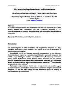
can predict whether two given values on the attribute (say a GMAT score of 610 and one of 590) will result in reliably different evaluations. There are many types of evaluability information people may have about an attribute. For illustrative purposes, below we examine three alternative scenarios. Scenario 1: When the evaluators have no evaluability information (except that greater numbers on the attribute are better). In SE of this case, any value on the attribute is extremely difficult or impossible to evaluate. That is, people have no idea whether a particular value is good or bad, let alone how good or how bad it is. We assume that the value will be evaluated, on average, as neutral, although it may be accompanied by a large variance. The evaluation function for the attribute will then be a flat line, as in Figure 1. In other words, those who see one option will give it roughly the same evaluation as those evaluating the other option. For example, suppose that the two applicants mentioned above are evaluated in SE by individuals who know nothing about GMAT scores other than greater numbers are better. Then those evaluating Applicant A will have about the same impression of that applicant as those evaluating Applicant B. We should note in passing that, in reality, people rarely possess no evaluability information about an attribute. For example, even people who know nothing about the range or distribution of GMAT scores may assume, on the basis of their knowledge of other tests, that GMAT scores should not be negative and that a score of 0 must be bad. As a result, the evaluation function is seldom absolutely flat. Scenario 2: When the evaluators know the neutral reference point (i.e., the evaluative zero-point) of the attribute. In this case, the evaluation function of the attribute in SE approximates a step function, as depicted in Figure 2. Any values above the reference point are considered good, and any values below the reference are considered bad. In this case, whether two attribute values will result in different evaluations in SE depends on whether they lie on the same side of the neutral reference point or straddle it. If the attribute values lie on the same side of the reference point, they will receive similar evaluations. If the attribute values are on opposite sides of the reference point (or one of the values coincides with the reference point), then the one above the reference point will be evaluated

Evaluation

O --

Figure 1. The evaluation function of an attribute when there is no evaluability information.

JOINT-SEPARATE EVALUATION REVERSALS more favorably than the other. For example, suppose that the individuals who evaluate the two applicants are told that the average GMAT score of applicants is 500, which they interpret as the neutral reference point (i.e., neither good nor bad). Then the two candidates will both be evaluated as good and will not be differentiated. On the other hand, if the evaluators are told that the average GMAT score is 600, then Applicant A (scored 610) will be evaluated as good and Applicant B (scored 590) as bad.3 Again, the above analysis is oversimplified. In reality, even if the evaluators only know the neutral reference point of the attribute, they will make speculations about the size and the meaning of the unit on the attribute. For example, people who are told that the average GMAT score is 600 may assume that a score like 601 is not very much different from 600 and not very good and that a score like 700 is quite different from 600 and must be quite good. As a result, the evaluation function is more likely to be S-shaped, rather than a strict step function. Scenario 3: When the evaluators are aware of the best possible and worst possible values of the attribute. In this scenario, the attribute is relatively easy to evaluate. The evaluation function will be monotonically increasing, as depicted in Figure 3. The general slope of the evaluation function, however, will be inversely related to the size of the range between the best and the worst values (e.g., Beattie & Baron, 1991; Mellers & Cook, 1994). In this condition, any two values on the attribute will create different impressions and result in different evaluations. The size of the difference depends on the size of the range between the best and the worst values. For example, Applicant A (with a score of 610) and Applicant B (with a score of 590) will be evaluated more differently if the evaluators are told that GMAT scores range from 550 to 650 than if they are told that GMAT scores range from 400 to 800. Qualifying the range effect, Beattie and Baron (1991) found that the range manipulation only affected the evaluations of unfamiliar stimuli. Consistent with the evaluability hypothesis, this finding suggests that providing or varying range information only affects the evaluation of attributes that would otherwise be hard to evaluate, namely, those for which the evaluators do not already have clear knowledge about the range or other evaluability information.

Evaluation

o --

Evaluation

o- -

W

Figure 2. The evaluation function of an attribute when there is neutral reference point information (R).

B

Figure 3. The evaluation function of an attribute when there is information about its worst value (W) and best value (B).

Again, in reality, the evaluation function in this condition will not be as linear as the one depicted in Figure 3. For example, people who are told that most applicants' GMAT scores range from 400 to 800 may treat the midpoint of the range, 600, as the neutral reference point. As a consequence, the evaluation function will be somewhat S-shaped, with its slope particularly steep around 600.

Evidence for the Preceding Analysis: The Score Study According to the preceding analysis, the evaluation function of an attribute varies predictably, depending on the evaluability information that people have. To test this proposition, we asked college students (N = 294) recruited from a large midwestern university to evaluate a hypothetical applicant to a university. In different experimental conditions, we varied evaluability information to see whether different applicant test scores would lead to different evaluations as a function of evaluability information. The questionnaire for this study included 12 between-subject versions. They constituted 3 Evaluability Conditions X 4 Score Conditions. In all versions, respondents were asked to imagine that they worked for the admissions office of a university, that their job was to evaluate prospective students' potential to succeed in college, and that they had just received the application of a foreign student named Jane. Participants were further told that Jane had taken an Academic Potential Exam (APE) in her country, that students in Jane's country are on average as intelligent as American students, that APE is a good measure of one's potential to succeed in college, and that the higher an APE score, the better. Corresponding to the three scenarios discussed in the previous section, the three evaluability versions for this study were (a) no information, (b) average score information, and (c) score range 3

R

579

Unless otherwise specified, we assume in this article that people evaluating Option A and people evaluating Option B in SE have the same evaluability information. For example, we assume that those evaluating Applicant A and those evaluating Applicant B have the same knowledge about GMAT scores.

HSEE, LOEWENSTEIN, BLOUNT, AND BAZERMAN

580

(i.e., best and worst score) information. The no-information version read You have no idea of the distribution of APE scores. You don't know what the average APE score, what the best APE score, or what the worst APE score is.

The average-score version read You don't have a clear idea of the distribution of APE scores. You know that the average APE score is 1,250, but you don't know what the best APE score or what the worst APE score is.

The score-range version read You don't have a clear idea of the distribution of APE scores. You know that the best APE score is 1,400 and the worst APE score is 1,100, but you don't know what the average APE score is.

Each of the three evaluability versions was crossed with four versions of Jane's APE score: 1,100, 1,200, 1,300, and 1,400, respectively. For example, the 1,100-version read Jane scored 1,100 on APE. The admissions office requires that you give a rating to each applicant even if you don't have all the information. Given what you know, how would you rate Jane's potential to succeed in college? Circle a number below:

-10 extremely poor

extremely good

neither good nor poor

The results, summarized in Table 1, lend support to the preceding analysis. In the no-information condition, the four scores formed almost a flat line, F(3, 96) = 1.51, ns. Planned comparisons indicate that the difference between any two score conditions was insignificant, suggesting that different scores created similar impressions. There is, however, a statistically insignificant yet distinctively positive slope across the four scores. This arises probably because even without any explicitly given evaluability information, the respondents used their knowledge about other tests to speculate on the missing information. In the average-score condition, the four scores formed an S-shaped function, with a steeper slope around the neutral reference point (the average score of 1,250). An F test across the four score conditions revealed a significant effect, F(3, 96) = 15.55, p < .01. Planned comparisons indicate that score 1,100 and score 1,200 were not evaluated significantly different, nor were scores 1,300 and 1,400, but either of the first two scores was judged significantly different from either of the latter two.

Table 1 Mean Evaluations of the Applicant in the Score Study Score of applicant Evaluability

1,100

1,200

1,300

1,400

No information Average score information only Score range information

5.13a 4.56a 3.04a

5.20a 4.71a 3.98b

5.54a 6.40b 6.52C

5.84a 6.84b 8.30d

Note. The ratings were made on a scale ranging from 0 (extremely poor) to 10 (extremely good). Means in the same row that do not share subscripts are significantly different from each other.

In the score-range condition, the four scores formed a steep upward slope, F(3, 97) = 73.83, p < .001. Planned comparisons show that each score was evaluated as significantly different from every other score in the predicted ordering. Note that the data are also indicative of an S-shape, suggesting that the respondents may have treated the midpoint of the range as a reference point and considered scores above this point to be generally good and scores below that point to be bad. In sum, the findings of this study show that the evaluation function of an attribute can migrate from a flat line to a steeply sloped function depending on the evaluability information the evaluators have.

Elaboration Several points deserve elaboration here. First, whether an attribute is easy or difficult to evaluate is not an intrinsic characteristic of the attribute. It is determined by the evaluability information the evaluators have about the attribute. Thus, the same attribute can be easy to evaluate in one context and for one group of evaluators but difficult to evaluate in another context or for other evaluators. For example, GMAT score is an easy-to-evaluate attribute for people familiar with the meaning of the score, its distribution, etc., but a difficult-to-evaluate attribute for other people. Second, an attribute can be difficult to evaluate even if its values are precisely given and people perfectly understand its meanings. For example, everybody knows what money is and how much a dollar is worth, but the monetary attribute of an option can be difficult to evaluate if the decision maker does not know the evaluability information for that attribute in the given context. Suppose, for instance, that a person on a trip to a foreign country has learned that a particular hotel room costs $50 a night and needs to judge the desirability of this price. If the person is not familiar with the hotel prices of that country, it will be difficult for him to evaluate whether $50 is a good or bad price. To say that an attribute is difficult to evaluate does not imply that the decision maker does not know its value but means that the decision maker has difficulty determining the desirability of its value in the given decision context. Finally, attributes with dichotomous values—such as whether a job candidate for an accountant position has a certified public accountant (CPA) license or not, or whether a vase being sold at a flea market is broken or not—are often easy to evaluate independently. People often know that these attributes have only two alternative values, and, even in SE when evaluators see only one value of the attribute (e.g., either with or without a CPA license), they know whether the value is the better or worse of the two. This is a special case of the situation where the evaluator has full knowledge of the evaluability information about the attribute. In several of the studies to be reviewed below, the easy-to-evaluate attribute is of this type.

Evaluability and JE/SE Reversals So far, we have only discussed the evaluability of a single attribute. In this section, we extend our analysis to options involving a trade-off across two attributes and explore how the evaluation hypothesis explains JE/SE reversals of these options.

JOINT-SEPARATE EVALUATION REVERSALS Consider two options, J and S, that involve a trade-off across Attribute x and Attribute y: Attribute x

Attribute y

Option J: Option S: where xs > *s and y} < ys (> denotes better than and < denotes worse than). According to the evaluability hypothesis, JE/SE reversals occur because one of the attributes is more difficult to evaluate than the other, and the relative impact of the difficult-to-evaluate attribute increases from SE to JE. Specifically, suppose that Attribute x is relatively difficult to evaluate independently and Attribute y is easy to evaluate independently. In SE, because Attribute x is difficult to evaluate, x, and xs will receive similar evaluations; as a result, this attribute will have little or no impact in differentiating the desirability of one option from that of the other. Because Attribute y is easy to evaluate, ys and ys will be evaluated differently; consequently, the evaluations of J and S in SE will be determined mainly by the values of Attribute y. Because ys > y,, S will tend to be evaluated more favorably than J. In JE, in contrast, people can easily compare the two options on an attribute-by-attribute basis (e.g., Russo & Dosher, 1983; Tversky, 1969). Through this comparison, people can easily tell which option is better on which attribute, regardless of whether the attribute is difficult or easy to evaluate in SE. Thus, both attributes will affect the evaluations of the target options. The above analysis indicates that, compared with SE, the impact of the difficult-to-evaluate attribute relative to that of the easy-toevaluate attribute increases in JE. In other words, the difficult-toevaluate attribute (x) benefits more from JE than the easy-toevaluate attribute (y). If Option S is favored in SE, and if Attribute x is important enough and/or the difference between xs and *s is large enough, then a JE/SE reversal will emerge, such that Option J will be favored over Option S in JE.

Evidence for the Preceding Analysis: Hiring Study and CD Changer Study Consider the hiring study (Hsee, 1996a) discussed earlier, involving a candidate with more KY programming experience and one with a higher GPA. Participants in this experiment were all college students, who knew which GPA values are good and which are bad, but they were unfamiliar with the criterion of KY programming experience. Thus, these participants had clear evaluability information for the GPA attribute but not for the KYprogramming-experience attribute. By definition, GPA was an easy-to-evaluate attribute, and KY programming experience was a relatively difficult-to-evaluate attribute. To assess whether our judgment of evaluability concurred with participants' own judgment, Hsee (1996a) asked those in each separate-evaluation condition, after they had made the WTP judgment, to indicate (a) whether they had any idea of how good the GPA of the candidate they had evaluated was and (b) whether they had any idea of how experienced with KY programming the candidate was. Their answers to each question could range from 1 (/ don't have any idea) to 4 (/ have a clear idea). The results confirmed our judgment that GPA was easier to evaluate than KY experience. The mean rating for GPA, 3.7, was significantly higher

581

than the mean rating of 2.1 for KY experience (t = 11.79, p < .001). According to the evaluability hypothesis, the difficult-toevaluate attribute has a greater impact relative to the easy-toevaluate attribute in JE than in SE. This is indeed what happened in the hiring study. As summarized earlier, the results indicate that the evaluations of the candidates in SE were determined primarily by the GPA attribute, and the evaluations in JE were influenced more heavily by the KY-experience attribute. It suggests that JE enabled the participants to compare the two candidates directly and thereby realize that the lower-GPA candidate had in fact completed many more programs than had the higher-GPA candidate.4 In most studies that demonstrate JE/SE reversals, whether an attribute is difficult or easy to evaluate independently is assumed. In the CD changer study described below, the evaluability of an attribute was manipulated empirically.5 As mentioned earlier, the evaluability hypothesis asserts that JE/SE reversals occur because one of the attributes of the stimulus objects is difficult to evaluate in SE, whereas the other attribute is relatively easy to evaluate. If this is correct, then a JE/SE reversal can be turned on or off by varying the relative evaluability of the attributes. To test this intuition, the CD changer study was designed as follows: It involved the evaluations of two CD changers (i.e., multiple compact disc players): CD Changer J: CD Changer S:

CD capacity Holds 5 CDs Holds 20 CDs

THD .003% .01%

It was explained to every participant that THD (total harmonic distortion) was an index of sound quality. The smaller the THD, the better the sound quality. The study consisted of two evaluability conditions: difficult/ easy and easy/easy. In the difficult/easy condition, participants received no other information about THD than described previously. As verified in subsequent questions (see below), THD was a difficult-to-evaluate attribute, and CD capacity was a relatively easy-to-evaluate attribute. Although most people know that less distortion is better, few know whether a given THD rating (e.g., .01%) is good or bad. On the other hand, most have some idea of how many CDs a CD changer could hold and whether a CD changer that can hold 5 CDs (or 20 CDs) is good or not. In the easy/easy condition, participants were provided with information about the effective range of the THD attribute. They were told, "For most CD changers on the market, THD ratings range from .002% (best) to .012% (worst)." This information was designed to make THD easier to evaluate independently. With this informa4 It should be noted that the distinction between difficult-to-evaluate and easy-to-evaluate attributes is different from that between proxy and fundamental attributes in decision analysis (e.g., Fischer, Damodaran, Laskey, & Lincoln, 1987). A proxy attribute is an indirect measure of a fundamental attribute—a factor that the decision maker is ultimately concerned about; for example, cholesterol level is a proxy attribute of one's health. A proxy attribute can be either easier or more difficult to evaluate than its fundamental attribute. For example, for people familiar with the meaning and the value distribution of cholesterol readings, the cholesterol attribute can be easier to evaluate than its fundamental attribute health; for people unfamiliar with cholesterol numbers, it can be very difficult to evaluate. 5 This study was originally reported in Hsee (1996a).

HSEE, LOEWENSTEIN, BLOUNT. AND BAZERMAN

582

tion, participants in the separate-evaluation conditions would have some idea where the given THD rating fell in the range and hence whether the rating was good or bad. In each of the evaluability conditions, participants (202 students from a large public university in the Midwest) were either presented with the information about both CD changers and evaluated both of them (JE), or presented with the information about one of the options and evaluated it alone (SE). In all conditions, the dependent variable was willingness-to-pay price. To ensure that the evaluability manipulation was effective, Hsee asked participants in the two separate-evaluation conditions, after they had indicated their WTP prices, (a) whether they had any idea of how good the THD rating of the CD changer was and (b) whether they had any idea of how large its CD capacity was. Answers to those questions ranged from 1 to 4, greater numbers indicating greater evaluability. The results confirmed the effectiveness of the evaluability manipulation. Mean evaluability scores for THD and CD capacity in the difficult/easy condition were 1.98 and 3.25, respectively, and in the easy/easy condition were 2.53 and 3.22. Planned comparisons revealed that evaluability scores for THD increased significantly from the difficult/easy condition to the easy/easy condition (t = 2.92, p < .01), but those for CD capacity remained the same. The main prediction for the study is that a JE/SE reversal was more likely to emerge in the difficult/easy condition than in the easy/easy condition. The results, summarized in Table 2, confirmed this prediction: In the difficult/easy condition, there was a significant JE/SE reversal (t = 3.32, p < .01), and the direction of the reversal was consistent with the evaluability hypothesis, implying that the difficult-to-evaluate attribute (THD) had a lesser relative impact in SE than in JE, and the easy-to-evaluate attribute (CD capacity) had a greater relative impact. In the easy/easy condition, the reversal disappeared (; < 1, ns). The fact that increasing the evaluability of the difficult-toevaluate attribute could eliminate the JE/SE reversal supports the evaluability hypothesis. It suggests that what drives this type of preference reversal is differential evaluability between the attributes.

Summary In this section, we first introduced the notion of evaluability and then used it to account for JE/SE reversals. The evaluability hypothesis, as our analysis shows, is not a post hoc speculation but a testable theory. First of all, the concept of evaluability was defined independently of the JE/SE-reversal effect, which it sub-

Table 2 Mean Willingness-to-Pay Values in the CD Changer Study Evaluability and evaluation mode Difficult/easy Joint Separate Easy/easy Joint Separate Note. CD = compact disc.

CD changer J

CD changer S

$228 $212

$204 $256

$222 $222

$186 $177

sequently explained. Moreover, we presented evidence of independent measures of evaluability and showed that participants' judgments of evaluability coincided with ours and predicted the observed reversals. Finally, in one study we empirically manipulated evaluability and demonstrated that this manipulation could turn the JE/SE reversal on or off in the direction predicted by the evaluability hypothesis.

Review and Explanation of JE/SE Reversals JE/SE reversals have been documented in diverse contexts. All of the findings involve pairs of options where one option is favored in JE and the other is favored in SE. Within this shared structure, JE/SE reversals can be classified into three types. In one type, the two options belong to the same category (e.g., both options are CD players), they share well-defined attributes (e.g., sound quality and CD capacity), and they involve explicit trade-offs along those attributes. All of the examples shown so far are of this type. In the second type of JE/SE reversal, the options also belong to the same category (just as in the first type), but they do not share welldefined attributes and do not involve explicit trade-offs. In the third type of JE/SE reversal, the options are from different categories. In what follows, we provide examples of each type of reversal and show how the evaluability hypothesis can be used to explain the finding.

JE/SE Reversals for Options From the Same Category and With Explicit Trade-Offs All of the JE/SE reversals discussed so far belong to this type. Here, the two options are from the same category (e.g., both are job candidates for a programmer position), and they involve an explicit trade-off along two attributes (e.g., GPA and programming experience). For this type of reversal, the evaluability hypothesis provides a straightforward explanation. In the previous section, we already examined how the evaluability hypothesis explains the result of the programmer-hiring study. The same analysis can be applied to Bazerman et al.'s (1992) self-neighbor study. Recall that in JE of this study the option that would give $600 to oneself and $800 to the neighbor (Option J) was favored over the option that would give $500 to both oneself and the neighbor (Option S), but in SE the pattern was reversed. The two options can be interpreted as involving a trade-off across the following two attributes: Option J: Option S:

Payoff to self $600 $500

Equality between self and neighbor Unequal Equal

Payoffs to self, we believe, were difficult to evaluate in SE because, lacking a comparison, respondents would not know how good a given settlement was. In contrast, whether or not the amount awarded to self was equal to the amount awarded to the neighbor was easy to evaluate. Most people, we surmise, would find an unequal treatment (especially when it is in favor of the other party) highly unattractive and would find an equal treatment neutral or positive. That is why the rank order of the two options in SE was determined primarily by the equality (equal versus unequal treatment) attribute. In JE, the payoff-to-self attribute was made easier to evaluate by the fact that the decision maker could compare the two values directly. On the other hand, the equality

JOINT-SEPARATE EVALUATION REVERSALS attribute, which was already easy to evaluate in SE, would not benefit as much from JE. That is why the payoff-to-self attribute loomed larger and led to a reversal in JE. Bazerman, Schroth, Shah, Diekmann, and Tenbrunsel (1994) obtained similar preference reversals with hypothetical job offers for MBA students that differed in terms of payoffs to oneself and equality or procedural justice in the company.6 Blount and Bazerman (1996) showed inconsistent evaluations of absolute versus comparative payoffs in recruiting participants for an experiment. These findings can be analyzed in the same way as Bazerman et al.'s (1992) preference reversal findings.7 Interested in trade-offs between absolute amount of income and temporal trend of income, Hsee (1993) solicited joint and separate evaluations of two hypothetical salary options, one with a higher absolute amount but a decreasing trend over a fixed 4-year period (Option J) and the other with a lower absolute amount but an increasing trend (Option S). The results revealed a JE/SE reversal: In JE, respondents slightly preferred the higher absolute-salary option, but in SE, the increasing-trend option was favored. Again, this result can be explained by evaluability. In SE, the absolute amount of earnings was difficult to evaluate, but whether the salary increased or decreased over time would elicit distinct feelings: People feel happy with improving trends and feel dejected with worsening trends, as shown in numerous recent studies (e.g., Ariely, 1998; Hsee & Abelson, 1991; Hsee, Salovey, & Abelson, 1994; Kahneman, Fredrickson, Schreiber, & Redelmeier, 1993; Loewenstein & Prelec, 1993; Loewenstein & Sicherman, 1991). In JE, the difference in absolute amount of earnings between the options became transparent and therefore loomed larger. In a more recent study, Hsee (1996a) observed a JE/SE reversal in WTP for two consumer products. Participants were asked to assume that they were a music major looking for a music dictionary in a used book store. They were provided the information about and indicated their WTP for either both or one of the following dictionaries: Dictionary J:

# of entries 20,000

Dictionary S:

10,000

Any defects? Yes, the cover is torn; otherwise it's like new. No, it's like new.

In JE, Dictionary J received higher WTP values, but in SE, Dictionary S enjoyed higher WTP values. The evaluability hypothesis also provides a ready explanation for the results. In SE, most respondents, who were not familiar with the evaluability information of music dictionary entries, would not know how to evaluate the desirability of a dictionary with 20,000 (or 10,000) entries. In contrast, even without something to compare it to, people would find a defective dictionary unappealing and a new-looking dictionary appealing. Therefore, we believe that the entry attribute was difficult to evaluate in SE and the defect attribute relatively easy to evaluate. This explains why in SE the rank order of WTPs for the two dictionaries was determined by the defect attribute. In JE, it was easy for people to realize that Dictionary J was twice as comprehensive, thus prompting them to assign a higher value to that dictionary. Lowenthal (1993) documented a similar JE/SE reversal in a rather different context. Interested in voting behavior, she created hypothetical congressional races between candidates who were

583

similar except for two dimensions. For example, consider the following two candidates: Jobs to be created Candidate J: 5000 jobs Candidate S: 1000 jobs

Personal history Convicted of misdemeanor Clean

In JE, participants voted for Candidate J, but, when asked to evaluate the candidates separately, participants rated Candidate S more favorably. For most respondents, who knew little about employment statistics, whether a candidate could bring 5,000 jobs or 1,000 jobs would be difficult to evaluate in isolation, but a candidate convicted of a misdemeanor would easily be perceived as unappealing and a candidate with a clean history as good. The direction of the reversal observed in the study is consistent with the evaluability hypothesis, suggesting that the personal history attribute had a greater impact in SE, and the job attribute loomed larger in JE.

JE/SE Reversals for Options From the Same Category but Without Explicit Trade-Offs Sometimes, JE/SE reversals occur with options that do not present explicit trade-offs between attributes. Instead, one option apparently dominates the other. In a recent study, Hsee (1998) asked students to imagine that they were relaxing on a beach by Lake Michigan and were in the mood for some ice cream. They were assigned to either the joint-evaluation or the separate-evaluation condition. Those in the joint-evaluation condition were told that there were two vendors selling Haagen Dazs ice cream by the cup on the beach. Vendor J used a 10 oz. cup and put 8 oz. of ice cream in it, and Vendor S used a 5 oz. cup and put 7 oz. of ice cream in it. Respondents saw drawings of the two servings and were asked how much they were willing to pay for a serving by each vendor. Respondents in each separate evaluation condition were told about and saw the drawing of only one vendor's serving, and they indicated how much they were willing to pay for a serving by that vendor. Note that, objectively speaking, Vendor J's serving dominated Vendor S's, because it had more ice cream (and also offered a larger cup). However, J's serving was underfilled, and S's serving was overfilled. The results revealed a JE/SE reversal: In JE, people were willing to pay more for Vendor J's serving, but in SE, they were willing to pay more for Vendor S's serving. In another experiment, Hsee (1998) asked participants to indicate their WTP prices for one or both of the following dinnerware sets being sold as a clearance item in a store:

Dinner plates: Soup/salad bowls:

Set J (includes 40 pcs) 8, in good condition 8, in good condition

Set S (includes 24 pcs) 8, in good condition 8, in good condition

6 Even in SE of these studies, the participants (who were MBA students) should have some idea of the distribution information for the salary attribute, and therefore, the salaries were not difficult to evaluate in its absolute sense. However, we suggest that JE provided more information about the salary attribute than SE, and, consequently, the salaries may have been even more easy to evaluate in JE than in SE. 7 Bazerman et al. (1998) had an alternative explanation for these results, which we discuss later.

584 Dessert plates: Cups: Saucers:

HSEE, LOEWENSTEIN, BLOUNT, AND BAZERMAN

8, in good condition 8, 2 of which are broken 8, 7 of which are broken

8, in good condition

Problem S:

Note that Set J contained all the pieces contained in Set S, plus 6 more intact cups and 1 more intact saucer. Again, there was a JE/SE reversal. In JE, respondents were willing to pay more for Set J. In SE, they were willing to pay more for Set S, although it was the inferior option. Although the options in these studies do not involve explicit trade-offs along well-defined attributes, the findings can still be accounted for by the evaluability hypothesis. In the ice cream study, the difference between the two servings can be reinterpreted as varying on two attributes: the absolute amount of ice cream a serving contained and whether the serving was overfilled or underfilled. Thus, the two servings can be described as follows: Serving J: Serving S:

Amount of ice cream 8 02. 7oz.

Filling Underfilled Overfilled

In SE, it was probably difficult to evaluate the desirability of a given amount of ice cream (7 oz. or 8 oz.), but the filling attribute was easier to evaluate: An underfilled serving was certainly bad and an overfilled serving good. According to the evaluability hypothesis, the filling attribute would be the primary factor to differentiate the evaluations of the two servings in SE, but in JE, people could see that Serving J contained more ice cream than Serving S and make their judgments accordingly. The results are consistent with these predictions. To see how the evaluability hypothesis applies to the dinnerware study, let us rewrite the differences between the dinnerware sets as follows: SetJ: Set S:

# of intact pieces 31 24

Problem J:

Integrity of the set Incomplete Complete

In SE, the desirability of a certain number of intact pieces (31 or 24) was probably rather difficult to evaluate (especially for students who were unfamiliar with dinnerware). On the other hand, the integrity of a set was probably much easier to evaluate: A set with broken pieces was certainly undesirable, and a complete set was desirable. Thus, the evaluability hypothesis would expect the intact set (S) to be favored in SE. In JE, the respondents could easily compare the sets and thereby would realize that Set J dominated Set S. Again, the results are consistent with these expectations.

JE/SE Reversals for Options From Different Categories In the studies reviewed so far, the options to be evaluated are always from the same category. JE/SE reversals have also been found between the evaluations of apparently unrelated options. Kahneman and Ritov (1994) observed a JE/SE reversal in an investigation of what they called the headline method. They presented participants with headlines describing problems from different categories and asked them how much they were willing to contribute to solving these problems. Consider the following, for example:

Skin cancer from sun exposure common among farm workers. Several Australian mammal species nearly wiped out by hunters.

It was found that in JE, respondents were willing to make a greater contribution to Problem J, and in SE, they were willing to make a greater contribution to Problem S. In a more recent study, Kahneman, Ritov, and Schkade (in press) studied people's reactions to two problems: Problem J: Multiple myeloma among the elderly. Problem S: Cyanide fishing in coral reefs around Asia. Again, there was a JE/SE reversal: In JE, people considered the disease issue (J) to be more important and also expected greater satisfaction from making a contribution to that issue. In SE, however, the reverse was true. In an experiment conducted by Irwin, Slovic, Lichtenstein, and McClelland (1993), respondents were asked to evaluate problems such as: Problem J: Improving the air quality in Denver. Problem S: Adding a VCR to your TV. When asked to select in pairwise comparisons between those options (JE), respondents overwhelmingly opted for improving the air quality. When those options were presented separately (SE), most respondents were willing to pay more for upgrading their TV. The main difference between these effects and the JE/SE reversals reviewed previously is that in these studies, the stimulus options are from unrelated categories. For example, in Kahneman et al.'s (in press) study, multiple myeloma is a human health problem, and cyanide fishing is an ecological problem. Our explanation of these results requires both norm theory (Kahneman & Miller, 1986) and the evaluability hypothesis. Take Kahneman et al.'s (in press) study, for example. In SE, the absolute importance of either problem is difficult to evaluate independently. People do not have much preexisting evaluability information for either multiple myeloma or cyanide fishing. According to norm theory, when evaluating an object, people often think about the norm of the category to which the object belongs and judge the importance of that object relative to the category norm. More specifically, norm theory suggests that, when evaluating multiple myeloma, participants would evoke the norm of the human-healthproblem category, and, when evaluating cyanide fishing, they would evoke the norm of the ecological-problem category. These evoked category norms essentially served as the evaluability information for judging the importance of each problem in SE. According to Kahneman et al., multiple myeloma is unimportant relative to the typical or normative human health problem, and cyanide fishing is important relative to the typical or normative ecological problem. In summary, the differences between Problems J (multiple myeloma) and S (cyanide fishing) in Kahneman et al.'s (in press) study can be considered as varying on two attributes: their absolute importance and their relative importance within their respective category.

JOINT-SEPARATE EVALUATION REVERSALS

Problem J: Problem S:

Absolute importance Hard to evaluate Hard to evaluate

Relative importance within category Unimportant Important

The absolute importance of each problem is difficult to judge independently, but the relative importance of each problem within its given category (i.e., relative to the category norm) is easy to evaluate. That explains why cyanide fishing was considered more important in SE. In JE, people could compare one problem with the other, and, through this comparison, they would recognize that a human health problem (J) must be more important than an ecological problem (S), hence assigning a higher WTP value to multiple myeloma. A similar analysis can be applied to Kahneman and Ritov's (1994) farmer/mammal study and Irwin et al.'s (1993) VCR/air quality study.8 The evaluability hypothesis and norm theory are not rival explanations. Instead, they complement each other to explain the above findings. Norm theory describes how category norms are evoked. The evaluability hypothesis describes how differential evaluability information can lead to JE/SE reversals. The linkage between the two theories is that, in all of the studies discussed in this section, the evaluability information is the category norm of the option under evaluation. Note that the structure of the problems discussed above is indeed quite similar to that of the ice cream study analyzed in the previous section. In the ice cream study, the absolute amount of ice cream is difficult to evaluate independently, but the amount of ice cream relative to the cup size is easy to evaluate. In Kahneman et al.'s (in press) health/ecological problem study, the absolute importance of each problem is difficult to evaluate independently, but the importance of each problem relative to the norm of its given category is easy to evaluate. More generally, the absolute value of an option is often hard to evaluate independently, but its relative position within a given category is usually easier to evaluate because the category serves as the evaluability information. As a result, a high-position member in a low category is often valued more favorably than a low-position member in a high category. Another study pertinent to the above proposition is reported in Hsee (1998). Students were asked to assume that they had received a graduation gift from a friend and to judge the generosity of the gift giver. For half of the students, the gift was a $45 wool scarf from a department store that carried wool scarves ranging in price from $5 to $50. For the other half of the students, the gift was a $55 wool coat from a department store that carried wool coats ranging in price from $50 to $500. Even though the $55 coat was certainly more expensive, those receiving the scarf considered their gift giver to be significantly more generous. These results can be explained in the same way as the ice cream study and the health/ecological problem study. The absolute price of a gift ($45 or $55) is difficult to evaluate in SE. However, whether the given gift is at the low end or high end of its respective product category is easy to evaluate in SE. The $45 scarf is at the top of the scarf category, and the $55 coat is near the bottom of the coat category. Therefore, the scarf appears more expensive and its giver more generous.

585

Summary In this section, we have reviewed recent research findings that document JE/SE reversals in diverse domains of decision making. They include JE/SE reversals between options that involve explicit trade-offs along well-defined attributes (e.g., the programmerhiring study), between options that belong to the same category but do not involve explicit trade-offs (e.g., the ice cream study), and between options that come from unrelated categories (e.g., the health/ecological problem study. We have shown that the evaluability hypothesis provides a simple and unifying explanation for all of these seemingly unrelated findings. In the next section, we discuss how the evaluability hypothesis differs from existing explanations of conventionally studied preference reversals.

Evaluability and Other Explanations for Preference Reversals Although the term preference reversal can be used to describe many documented violations of normative axioms, such as Allais's Paradox (Allais, 1953) and intransitivity (e.g., May, 1954; Tversky, 1969), the concept of preference reversal gained its recognition in decision research with the P-bet/$-bet research of Lichtenstein and Slovic (1971) and subsequently of Grether and Plott (1979). The P-bet offers a high likelihood of winning a small amount of money, whereas the $-bet offers a low probability of winning a larger amount of money. The P-bet is often preferred when participants are asked to make a choice between the two bets, and the $-bet is favored when participants are asked to indicate a minimum selling price for each bet. The standard explanation for this type of preference reversal is the compatibility principle (Slovic, Griffin, & Tversky, 1990). According to this principle, the weight given to an attribute is greater when it matches the evaluation scale than when it does not. For example, attributes involving monetary values, such as monetary payoff, loom larger if preferences are elicited in terms of price than in terms of choice. This principle serves as a compelling explanation for the choice-pricing preference reversal and many other related choice-judgment reversals (see Schkade & Johnson, 1989, for process data that supports the scale compatibility explanation of choice-pricing reversals). The compatibility principle is concerned with preference reversals involving different evaluation scales as opposed to those with different evaluation modes. Another type of commonly studied preference reversal occurs between choice and matching (Tversky et al., 1988; for more recent studies, see Coupey, Irwin, & Payne, 1998). For example, consider a study by Tversky et al. (1988) involving two hypothetical job candidates for a production engineer position: Candidate A had a technical score of 86 and a human relations score of 76; Candidate B had a technical score of 78 and a human relations score of 91. In choice, participants were asked to choose between 8

There is another possible interpretation of Irwin et al.'s (1993) results. When making a choice between worse air pollution in Denver and upgrading their own appliance, people may have felt it would be selfish to benefit themselves trivially at the expense of all Denver residents. When they were asked to put a monetary value of clean air, no such direct tradeoff is implied, and they may have thought about the benefit of clean air to only themselves.

586

HSEE, LOEWENSTEIN, BLOUNT, AND BAZERMAN

the two candidates, and most chose Candidate A. In matching, participants were presented with the same alternatives, but some information about one of the candidates was missing. The participants' task was to fill in that information to make the two alternatives equally attractive. Typically, the values respondents filled in implied that they would have preferred Candidate B had the information not been missing. To explain the preference reversal between choice and matching, Tversky et al. proposed the prominence principle, which states that the most prominent attribute in a multiattribute choice set is weighted more heavily in choice than in matching. In the example above, technical score was apparently the more important attribute, and, according to the prominence principle, it loomed larger in choice than in matching. Fischer and Hawkins (1993) extended the prominence principle by contending that the most prominent attribute looms larger in qualitative tasks (e.g., choice and strength-of-preference judgment) than in quantitative tasks (e.g., value-matching and monetaryequivalent value judgments). Although the prominence principle provides a good explanation for the standard choice-matching preference reversal, it does not readily apply to JE/SE reversals studied in the present research. In the choice-matching paradigm, both the choice task and the matching task are carried out in the JE mode, and the prominence principle explains how the relative weight of the attributes varies between tasks that involve different evaluation scales. JE/SE reversals, on the other hand, can take place even if the evaluation scale is held constant (e.g., about willingness to pay), and therefore they cannot be explained by theories that focus on differential evaluation scales. In addition, the prominence principle relies on difference in attribute prominence for preference reversals to occur. However, our research shows that a JE/SE reversal can be turned on or off even if the relative prominence of the attributes remains constant (e.g., in the CD-changer experiment previously reviewed). It suggests that for tasks that differ in evaluation modes, differential evaluability alone is sufficient to induce a preference reversal. The evaluability hypothesis is not, therefore, an alternative explanation to the prominence or compatibility principle; instead, they seek to explain different phenomena. Mellers and her associates (Mellers et al., 1992; Mellers, Ordonez, & Birnbaum, 1992) have a change-of-process theory to account for preference reversals between tasks involving different evaluation scales. It asserts that people using different evaluation scales (e.g., ratings versus prices) adopt different cognitive models when evaluating alternative risky options, thus leading to preference reversals between those options. Like the compatibility and the prominence principles, the change-of-process theory also relies on difference in evaluation scales to explain preference reversals and hence does not apply to the JE/SE reversals explored in the present research. Recently, Bazerman, Tenbrunsel, and Wade-Benzoni (1998) provided another explanation for some of the JE/SE reversals reviewed earlier, which they termed the want/should proposition. In the series of studies involving options varying on payoffs to self and equality or fairness (e.g., Bazerman et al., 1992, 1994), Bazerman et al. (1998) suggest that the payoff attribute is a should attribute (i.e., a factor the respondents think they should consider) and the equality attribute is a want attribute (i.e., a factor that the respondents want to consider). They then explain these JE/SE reversals by proposing that should attributes loom larger in JE and want attributes loom larger in SE. That is presumably because SE

gives decision makers greater leeway to do what they are motivated to do rather than what they feel they should do; this proposition is consistent with the elastic justification notion posited in Hsee (1995, 1996b). We agree with Bazerman et al. (1998) that the want/should proposition is an appealing alternative explanation for the JE/SE reversals in those studies. However, it lacks several ingredients of a general explanation for JE/SE reversals. First, it is often difficult to know a priori which attributes are should attributes and which are want attributes. For example, in the programmer-hiring study, it is difficult to identify a priori whether GPA is the should attribute and programming experience is the want attribute, or vice versa. Further, the want/should proposition is silent about why a JE/SE reversal can be turned on or off by evaluability manipulation. Nevertheless, the want/should proposition provides a possible explanation for JE/SE reversals involving trade-offs between monetary payoffs and fairness. Further research is needed to determine whether those findings are caused by the want/should difference, by differential attribute evaluability, or by a combination of the two. Nowlis and Simonson (1997) documented robust preference reversals between a choice task and a rating task. In one experiment, for example, participants in the choice condition were presented with multiple products varying in price and brand and asked to choose one. Participants in the rating condition were also presented with those multiple products simultaneously and asked to rate their purchase intention on a rating scale. For the choice group, low-price/low-quality products (e.g., a $139 Goldstar microwave oven) were preferred; in the rating group, high-price/ high-quality products (e.g., a $179 Panasonic microwave oven) were favored. These observations resemble the traditional choicejudgment reversal where the main difference between choice and judgment lies in evaluation scale, not evaluation mode. Nowlis and Simonson also showed that the preference reversal was not mitigated even when the participants were given information about the price range of the product, e.g., that the prices of microwaves range from $99 to $299. This result is not inconsistent with our research. Unlike attributes such as total harmonic distortion, which are extremely difficult to evaluate, the price of a microwave is familiar to most people. Adding range information to an alreadyfamiliar attribute, especially when the range is very large ($99 to $299) relative to the difference between the original stimulus values ($139 and $179), may in fact decrease, rather than increase, the impact of the attribute (e.g., Mellers & Cook, 1994). Nowlis and Simonson's work is complementary to our research. Their findings corroborate most traditional choice-judgment preference reversal studies by showing that a difference in evaluation scale alone is sufficient to produce preference reversals. Their work further indicates that evaluation-scale-based preference reversals are different from JE/SE reversals and cannot be readily explained by the evaluability hypothesis. Nowlis and Simonson explained their results in terms of compatibility between type of response (choice versus rating) and type of attribute (comparative versus enriched). Their explanation is an extension of the compatibility principle (Slovic et al., 1990). We conclude this section with two caveats. First, we have made a clear distinction between evaluation mode and evaluation scale and have shown that a JE/SE reversal can occur even if the evaluation scale is held constant. However, evaluation mode and evaluation scale are often naturally confounded in real-world de-

JOINT-SEPARATE EVALUATION REVERSALS cision making. When people are called on to decide which of two options to accept (i.e., a choice task), they are inevitably in the JE mode, comparing the two options side by side. In other words, choice is a special case of JE. On the other hand, when people consider how much they are willing to sell an item for, they are typically in the SE mode, focusing primarily on the target item alone (although they need not be). In this example, choice is confounded with JE, and pricing is confounded with SE. As a result, explanations for these reversals require a combination of the evaluability hypothesis and traditional theories for the evaluation scale effect, such as compatibility and prominence. Second, the present article focuses only on one type of inconsistency between JE and SE—preference reversal. In a JE/SE reversal, the desirability of one option relative to the other changes between the evaluation modes. Hsee and Leclerc (1998) recently explored another type of JE/SE inconsistency where the desirability of both options changes between the evaluation modes, although their relative desirability remains unchanged, so there is no preference reversal. Specifically, they found that the desirability of low-quality products increased from SE to JE, whereas the desirability of high-quality products decreased from SE to JE. Those findings are not driven by differential attribute evaluability and are beyond the realm of this article (see Hsee & Leclerc, 1998, for details).

Implications of the Evaluability Hypothesis Although the evaluability hypothesis is proposed originally to explain JE/SE reversals, it is potentially a more general theory. It describes how people make judgments and decisions when they do or do not have sufficient evaluability information. As such, the evaluability hypothesis has implications for phenomena beyond preference reversals. To illustrate, let us examine how this hypothesis explains why people are sometimes grossly insensitive to normatively important variables. In a dramatic demonstration of this insensitivity, Desvousges et al. (1992; cited in Kahneman et al., in press) asked respondents how much they were willing to pay to save x number of migrating birds dying in uncovered oil ponds every year, x varied across different groups of respondents; it was either 2,000, 20,000, or 200,000. Normatively speaking, the number of bird deaths (x) should be an important determinant of respondents' WTP, but it had little effect. Mean WTP was about the same ($80, $78, and $88, respectively) for saving 2,000 birds, 20,000 birds, or 200,000 birds. This apparent anomalous result is highly consistent with the evaluability hypothesis. In the Desvousges et al. (1992) study, respondents had no evaluability information about bird death tolls, making this attribute extremely difficult to evaluate independently. According to the evaluability hypothesis, an attribute would have no power to differentiate the evaluations of the target options if the evaluators have no evaluability information about the attribute; the evaluation function in this condition resembles a flat line. That is why WTP values were virtually the same for the different birddeath conditions. This result is very similar to the finding in the no-information condition of the previously described score study, whereas ratings for the foreign student were virtually the same among the different score conditions. Although it was not tested in the Desvousges et al. (1992) study, the evaluability hypothesis would predict that if the three birddeath conditions had been evaluated by the same group of partic-

587

ipants in a JE mode, or if the respondents had received more evaluability information about endangered birds, then the bird death numbers would have had a greater effect on WTP. Consistent with this prediction, Frederick and Fischhoff (1998) observed much greater scale sensitivity in a within-subject study, in which respondents were asked to evaluate several goods that differed in scale, than in a between-subject design, in which different participants evaluated each of the goods. The evaluability hypothesis can also explain why people in SE are often insensitive to variation in the value they are actually concerned about and sensitive only to variation in the proportion of that value to a certain base number. For example, suppose that there are two environmental protection programs: Program J is designed to save birds in a forest where there are 50,000 endangered birds; it can save 20% of these birds. Program S is designed to save birds in a forest where there are 5,000 endangered birds; it can save 80% of these birds. Although Program J can save 10,000 birds (i.e., 20% X 50,000), whereas Program S can save only 4,000 birds (i.e., 80% X 5,000), chances are that Program S will be favored in SE. This example is a variant of Fetherstonhaugh, Slovic, Johnson, and Friedrich's (1997) finding that programs expected to save a given number of lives received greater support if the number of lives at risk was small than if it was large (see also Baron, 1997, and Jenni & Loewenstein, 1997, for similar results). Baron (1997) showed that the high sensitivity to relative (rather than absolute) risk was most pronounced in studies using a between-subject (SE) design and was mitigated in a study using a JE mode. This finding is consistent with the evaluability hypothesis. Note that the structure of the options in the example above is parallel to that in the ice cream study. The actual number of birds the program can save is like the actual amount of ice cream; it is the main value of concern. The size of the forest is like the size of the cup; it is a base number. The proportion of birds a program can save is like the filling attribute; it reflects the relationship between the value of concern and the base number. As in the ice cream study, the evaluability hypothesis predicts that, in SE, Program S would be considered more favorably than Program J. The reason is simple: The actual value of concern—in this case, how many birds the program can save—is difficult to evaluate independently. In contrast, the proportion attribute—whether a program can save 20% or 80% of the birds in a forest—is relatively easy to evaluate; 20% seems small and 80% seems large. Another finding that may be related to evaluability is the observation by Fox and Tversky (1995) that the ambiguity aversion effect (the tendency to prefer gambles with known probabilities to those with unknown probabilities) occurred only in JE and not in SE. Fox and Tversky interpreted their results as showing that ambiguity aversion is an inherently comparative phenomenon, a hypothesis they called comparative ignorance. However, their findings can also be explained in terms of evaluability. Like many other attributes reviewed earlier, whether a gamble is ambiguous or not may be easier to evaluate in JE than in SE. Fox and Tversky sought to demonstrate that the effect was specific to ambiguity by showing (in their Study 5) that such a reversal did not occur with two gambles that differed in their probability of winning rather than ambiguity (one had a high probability of winning and the other had a small probability of winning). However, this result is

588

HSEE, LOEWENSTEIN, BLOUNT, AND BAZERMAN

consistent with an evaluability interpretation because there is no reason to think that probability was particularly difficult to evaluate even in SE. Ambiguity aversion may, in fact, be an inherently comparative phenomenon, but it is only one of many attributes that receive greater weight in JE than in SE. Marsh (1984) summarizes a variety of findings from Dr. Fox studies of student evaluation in which students gave higher teaching ratings to slick lecturers who presented little substance than to duller lecturers who covered material in depth. Marsh argues that the findings may reflect a process that is quite analogous to the evaluability hypothesis: Finally, I would like to suggest a counter-explanation for some of the Dr. Fox findings. . . . Some instructor characteristics such as expressiveness and speech clarity can be judged in isolation because a frame of reference has probably been established through prior experience, and these characteristics do influence student ratings. For other characteristics such as content coverage, external frames of reference are not so well defined. . . . If students were asked to compare high and low content lectures... I predict that their responses would more accurately reflect the content manipulation. (1984, p. 745)

Let us conclude this article with a discussion of a rather metaphysical question: Which evaluation mode is better—joint or separate? The long-standing advice for people to always consider the alternatives in decision making (e.g., Baron, 1988; Janis & Mann, 1977) implies that JE is always better than SE. However, we believe that the answer is not that simple. We agree that, in most cases, JE is better because it makes explicit the trade-offs underlying the options. This point is particularly evident if we consider the ice cream and the dinnerware studies (Hsee, 1998), where JE led to a preference for the objectively dominant option, and SE led to a preference for the objectively inferior option. The idea that JE is better than SE is consistent with previous findings, showing that people often arrive at better decisions if they have considered alternatives than if they have not. For example, Frisch and Jones (1993) conducted a retrospective study in which participants reported a recent decision that resulted in either a very bad outcome or a very good outcome. Participants then responded to a battery of questions about the decision processes that had led to each of these decisions. Although acknowledging that good decisions can result in bad outcomes and vice versa, their study was premised on the idea that, on average, good decisions tend to result in better outcomes than do bad decisions. The single strongest difference in process between decisions that turned out well and decisions that turned out badly was whether participants had considered alternative courses of action before deciding. However, JE is not unconditionally better than SE. In JE, people may be overly sensitive to the difference between the alternative options on a certain attribute, whereas this difference may not even be detectable in SE. If the ultimate consumption of an option is in the SE mode, then the preference elicited in JE may be inconsistent with one's actual consumption experience. The preceding point has important implications for discrepancies between decision and experience utilities (e.g., Kahneman & Snell, 1990, 1992). It is probably not difficult for us to recall times when we decided to choose one option over another, but we ended up being unhappy with the option we chose and would probably be happier had we chosen the forgone option. Such decision-experience inconsistencies permeate

consumer decisions, career decisions, and marital decisions, to name just a few. There have been a number of explanations for these inconsistencies, including, for example, changing tastes (March, 1978), inability to predict adaptation (Loewenstein & Frederick, 1997), differential arousal states (Loewenstein, 1996), and the prominence and the compatibility principles (Tversky & Griffin, 1991). We believe that JE/SE reversals should be added to the list of important sources of discrepancies between decision utility and experience utility. At the time of the decision, an individual is typically exposed to all possible alternatives, and so the evaluation mode is JE. At the time of experiencing the consequence of the option one has chosen, the individual is usually in SE. For example, when a person buys a piano in a musical instrument store, there are typically myriad models for her to compare and choose from (JE). However, after she buys a piano, and when she uses it at home—that is, plays it, looks at it, etc., she is exposed mostly to that particular piano alone (SE). Just as different attributes have different relative impact in JE than in SE, so will these attributes have different relative impact in the decision phase than in the consumption phase. To illustrate, consider an audio store that carries two models of loudspeakers of equal price. One model looks attractive and the other looks ugly. The ugly-looking model has a slightly lower distortion level and thus sounds slightly better. For most nonaudiophile consumers, the appearance of a speaker is easy to evaluate independently, and its sound quality is not. The sound quality of a speaker can only be appreciated when it is compared directly with another speaker. When consumers are in the store and are making a purchase decision, they are typically in JE; they can easily compare one model against the other. Through the comparison, the difference in sound quality becomes salient. In this situation, many people may end up buying the better-sounding but ugly-looking model. However, once people have purchased a set of speakers and brought them home, they are usually in the SE mode; they enjoy (or suffer with) whatever they have bought and do not actively compare it with the forgone alternative. In SE, the difference in sound quality between the ugly and the attractive models may not make any difference in one's consumption experience, but the difference in appearance may. Thus, people who bought the ugly model may not enjoy its sound quality any more than those who bought the good-looking model, but the former group of consumers may be constantly bothered by the ugly appearance of the speakers they bought.9 The moral of this example is that when making decisions, people may put too much weight on difficultto-evaluate attributes and be too concerned with differences between options on those attributes that will make little or no 9 Two qualifications about this example: First, sometimes people may also find themselves in JE during the consumption phase, when, for example, their neighbor happens to have bought the alternative model and they can easily compare theirs with their neighbor's. However, we believe that in most circumstances, the evaluation mode at the consumption phase is much closer to the SE end on the JE-SE continuum than is the evaluation mode at the purchase phase. Second, our analysis here applies mainly to decisions whose main purpose is to optimize consumption experience. However, sometimes the decision maker has other goals in mind, and/or the construct of consumption experience does not capture the whole scope of costs and benefits of an option. Under those circumstances, our analysis may not apply.

JOINT-SEPARATE EVALUATION REVERSALS difference in SE, hence little or no difference in actual consumption experience. Shafir (in press) argues that the distinction between joint and separate evaluation has even wider implications. He proposes that guidelines and policies arise from joint evaluation of alternative scenarios, but events in the real world, to which these guidelines and policies are supposed to apply, usually present themselves one at a time. Because of inconsistencies between joint and separate evaluation, these guidelines and policies may not optimally serve these events in the real world. In short, people make judgments and decisions in one of two primary evaluation modes—joint or separate. Our research shows that evaluations in these modes can yield inconsistent preferences. In addition, as just discussed, people do not always evaluate objects in the mode that is most likely to result in the best consumption experience. Which mode people use depends on whether they have a ready alternative with which to compare. When there is an available alternative option, people often naturally engage in JE. When no alternatives are present, people do not automatically think of alternatives (e.g., Gettys, Pliske, Manning, & Casey, 1987; Legrenzi, Girotto, & Johnson-Laird, 1993), and they engage in SE. Which mode is better for the consumer is a different issue. It depends on the goal people intend to achieve through the decision. If the goal is to choose the objectively most valuable option, then JE is probably better. If the goal is to choose the option that will optimize one's consumption experience, and if consumption takes place in SE, then SE may prove better.

References Allais, P. M. (1953). The behavior of rational man in risk situations—A critique of the axioms and postulates of the American School. Econometrica, 21, 503-546. Ariely, D. (1998). Combining experiences over time: The effects of duration, intensity changes and on-papers line measurements on retrospective pain evaluation. Journal of Behavioral Decision Making, 11, 19-45. Baron, J. (1988). Thinking and deciding. New York: Cambridge University Press. Baron, J. (1997). Confusion of relative and absolute risk in valuation. Journal of Risk and Uncertainty, 14, 301-309. Bazerman, M. H., Loewenstein, G. F., & White, S. B. (1992). Reversals of preference in allocation decisions: Judging an alternative versus choosing among alternatives. Administrative Science Quarterly, 37, 220-240. Bazerman, M. H., Schroth, H. A., Shah, P. P., Diekmann, K. A., & Tenbrunsel, A. E. (1994). The inconsistent role of comparison others and procedural justice in reactions to hypothetical job descriptions: Implications for job acceptance decisions. Organizational Behavior and Human Decision Processes, 60, 326-352. Bazerman, M. H., Tenbrunsel, A., & Wade-Benzoni, K. (1998). Negotiating with yourself and losing: Understanding and managing competing internal preferences. Academy of Management Review, 23, 225-241. Beattie, J., & Baron, J. (1991). Investigating the effect of stimulus range on attribute. Journal of Experimental Psychology: Human Perception and Performance, 17, 571-585. Birnbaum, M. H. (1992). Issues in utility measurement. Organizational Behavior and Human Decision Processes, 52, 319-330. Blount, S., & Bazerman, M. H. (1996). The inconsistent evaluation of absolute versus comparative payoffs in labor supply and bargaining. Journal of Economic Behavior & Organization, 30, 227-240. Coupey, E., Irwin, J. R., & Payne, J. W. (1998). Product category familiarity and preference construction. Journal of Consumer Research, 24, 459_467. Coursey, D. L., Hovis, J. J., & Schulze, W. D. (1987). The disparity

589

between willingness to accept and willing to pay measures of value. Quarterly Journal of Economics, 102, 679-690. Desvousges, W., Johnson, R., Dunford, R., Boyle, K. J., Hudson, S., & Wilson, K. N. (1992). Measuring non-use damages using contingent valuation: An experimental evaluation accuracy. Research Triangle Institute Monograph, 92-1. Fetherstonhaugh, D., Slovic, P., Johnson, S. M., & Friedrich, J. (1997). Insensitivity to the value of human life: A study of psychophysical numbing. Journal of Risk and Uncertainty, 14, 283-300. Fischer, G. W., Damodaran, N., Laskey, K. B., & Lincoln, D. (1987). Preferences for proxy attributes. Management Science, 33, 198-214. Fischer, G. W., & Hawkins, S. A. (1993). Strategy compatibility, scale compatibility, and the prominence effect. Journal of Experimental Psychology: Human Perception and Performance, 19, 580-597. Fox, C. R., & Tversky, A. (1995). Ambiguity aversion and comparative ignorance. The Quarterly Journal of Economics, 110, 585-603. Frederick, S., & Fischoff, B. (1998). Scope (in)sensitivity in elicited valuations. Risk Decision and Policy, 3, 109-123. Frisch, D., & Jones, S. K. (1993). Assessing the accuracy of decisions. Theory and Psychology, 3, 115-135. Gettys, C. F., Pliske, R. M., Manning, C., & Casey, J. T. (1987). An evaluation of human act generation performance. Organizational Behavior and Human Decision Processes, 39, 23-51. Goldstein, W. M., & Einhorn, H. J. (1987). Expression theory and the preference reversal phenomena. Psychological Review, 94, 236-254. Grether, D. M., & Plott, C. R. (1979). Economic theory of choice and the preference reversal phenomenon. American Economic Review, 69, 623638. Hsee, C. K. (1993). When trend of monetary outcomes matters: Separate versus joint evaluation and judgment of feelings versus choice. Unpublished manuscript, The University of Chicago. Hsee, C. K. (1995). Elastic justification: How tempting but task-irrelevant factors influence decisions. Organizational Behavioral and Human Decision Process, 62, 330-337. Hsee, C. K. (1996a). The evaluability hypothesis: An explanation of preference reversals between joint and separate evaluations of alternatives. Organizational Behavior and Human Decision Processes, 46, 247-257. Hsee, C. K. (1996b). Elastic justification: How unjustifiable factors influence judgments. Organizational Behavior and Human Decision Processes, 66, 122-129. Hsee, C. K. (1998). Less is better: When low-value options are valued more highly than high-value options. Journal of Behavioral Decision Making, 11, 107-121. Hsee, C. K., & Abelson, R. P. (1991). The velocity relation: Satisfaction as a function of the first derivative of outcome over time. Journal of Personality and Social Psychology, 60, 341-347. Hsee, C. K., & Leclerc, F. (1998). Will products look more attractive when evaluated jointly or when evaluated separately? Journal of Consumer Research, 25, 175-186. Hsee, C. K., Salovey, P., & Abelson, R. P. (1994). The quasi-acceleration relation: Satisfaction as a function of the change in velocity of outcome over time. Journal of Experimental Social Psychology, 30, 96-111. Irwin, J. R. (1994). Buying/selling price preference reversals: Preference for environmental changes in buying versus selling modes. Organizational Behavior and Human Decision Processes, 60, 431-457. Irwin, J. R., Slovic, P., Lichtenstein, S., & McClelland, G. H. (1993). Preference reversals and the measurement of environmental values. Journal of Risk and Uncertainty, 6, 5-18. Janis, I. L., & Mann, L. (1977). Decision making: A psychological analysis of conflict, choice, and commitment. New York: Free Press. Jenni, K., & Loewenstein, G. (1997). Explaining the "identifiable victim effect," Journal of Risk and Uncertainty, 14, 235-257. Kahneman, D., Fredrickson, B. L., Schreiber, C. A., & Redelmeier, D. A.

590

HSEE, LOEWENSTEIN, BLOUNT, AND BAZERMAN

(1993). When more pain is preferred to less: Adding a better end. Psychological Science, 4, 401—405. Kahneman, D., Knetsch, J. L., & Thaler, R. H. (1990). Experimental tests of the endowment effect and the Coase theorem. Journal of Political Economy, 98, 1325-1348. Kahneman, D., & Miller, D. T. (1986). Norm theory: Comparing reality with its alternatives. Psychological Review, 93, 136-153. Kahneman, D., & Ritov, I. (1994). Determinants of stated willingness to pay for public goods: A study in the headline method. Journal of Risk and Uncertainty, 9, 5-38. Kahneman, D., Ritov, I., & Schkade, D. (in press). Economists have preferences; psychologists have attitudes: An analysis of dollar responses to public issues. In D. Kahneman & A. Tversky (Eds.), Choices, values and frames. New York: Cambridge University Press. Kahneman, D., & Snell, J. (1990). Predicting utility. In R. M. Hogarth (Ed.), Insights in decision making (pp. 295-311). Chicago: University of Chicago Press. Kahneman, D., & Snell, J. (1992). Predicting a changing taste: Do people know what they will like? Journal of Behavioral Decision Making, 5, 187-200. Knetsch, J. L., & Sinden, J. A. (1984). Willingness to pay and compensation demanded—Experimental evidence of an unexpected disparity in measures of value. Quarterly Journal of Economics, 99, 507-521. Legrenzi, P., Girotto, V., & Johnson-Laird, P. N. (1993). Focusing in reasoning and decision making. Cognition, 49, 37-66. Lichtenstein, S., & Slovic, P. (1971). Reversal of preferences between bids and choices in gambling decisions. Journal of Experimental Psychology, 89, 46-55. Loewenstein, G. (1996). Out of control: Visceral influences on behavior. Organizational Behavior and Human Decision Processes, 65, 272-292. Loewenstein, G., Blount, S., & Bazerman, M. H. (1993). Reversals of Preference Between Independent and Simultaneous Evaluation of Alternatives. Unpublished manuscript, Carnegie Mellon University, Pittsburgh, Pennsylvania. Loewenstein, G., & Frederick, S. (1997). Predicting reactions to environmental change. In M. Bazerman, D. Messick, A. Tenbrunsel, & K. Wade-Benzoni (Eds.), Psychological perspectives on the environment. San Francisco: New Lexington Press. Loewenstein, G., & Prelec, D. (1993). Preferences for sequences of outcomes. Psychological Review, 100, 91-108. Loewenstein, G., & Sicherman, N. (1991). Do workers prefer increasing wage profile? Journal of Labor Economics, 9, 67-84. Lowenthal, D. (1993). Preference reversals in candidate evaluation. Working paper. Carnegie Mellon University, Pittsburgh, Pennsylvania. March, J. (1978). Bounded rationality, ambiguity and the engineering of choice. Bell Journal of Economics, 9, 587-608. Marsh, H. W. (1984). Students' evaluations of university teaching: Dimensionality, reliability, validity, potential biases, and utility. Journal of Educational Psychology, 76, 707-754. May, K. O. (1954). Intransitivity, utility and the aggregation of preference patterns. Econometrica, 22, 1-13.

Mellers, B. A., Chang, S., Birnbaum, M. H., & Ordonez, L. D. (1992). Preferences, prices and ratings in risky decision making. Journal of Experimental Psychology: Human Perception and Performance, 18, 347-361. Mellers, B. A., & Cook, D. J. (1994). Tradeoffs depend on attribute range. Journal of Experimental Psychology: Human Perception and Performance, 20, 1055-1067. Mellers, B. A., Ordonez, L. D., & Birnbaum, M. H. (1992). A change-ofprocess theory for contextual effects and preference reversals in risky decision making. Organizational Behavior and Human Decision Processes, 52, 331-369. Nowlis, S. M., & Simonson, I. (1994). The context-dependency of attributes as a determinant of preference reversals between choices and judgments of purchase likelihood. Working paper. Stanford University, Palo Alto, California. Nowlis, S. M., & Simonson, I. (1997). Attribute-task compatibility as a determinant of consumer preference reversals. Journal of Marketing Research, 34, 205-218. Payne, J. W., Bettman, J. R., & Johnson, E. J. (1992). Behavioral decision research: A constructive processing perspective. Annual Review of Psychology, 43, 87-131. Russo, J. E., & Dosher, B. A. (1983). Strategies for multiattribute binary choice. Journal of Experimental Psychology: Learning, Memory, and Cognition, 9, 676-696. Schkade, D. A., & Johnson, E. J. (1989). Cognitive processes in preference reversals. Organizational Behavior and Human Decision Processes, 44, 203-231. Shafir, E. (1993). Choosing versus rejecting: Why some options are both better and worse than others. Memory & Cognition, 21, 546-556. Shafir, E. (in press). Cognition, intuition and policy guidelines. In R. Gowda & J. Fox (Eds.), Judgments, decisions and public policy. New York: Cambridge University Press. Slovic, P., Griffin, D., & Tversky, A. (1990). Compatibility effects in judgment and choice. In R. M. Hogarth (Ed.), Insights in decision making: Theory and applications (pp. 5-27). Chicago: University of Chicago. Tversky, A. (1969). Intransitivity of preferences. Psychological Review, 76, 31-48. Tversky, A., & Griffin, D. (1991). Endowment and contrast in judgments of well-being. In F. Strack, M. Argyle, & N. Schwartz (Eds.), Subjective well-being: An interdisciplinary perspective (Vol. 21, pp. 101-118). Oxford, England: Pergamon Press. Tversky, A., Sattath, S., & Slovic, P. (1988). Contingent weighting in judgment and choice. Psychological Review, 95, 371-384.

Received January 23, 1998 Revision received March 5, 1999 Accepted March 5, 1999