Advanced Drug Delivery Reviews 54 (2002) 355–366 www.elsevier.com / locate / drugdeliv
Prediction of drug solubility from structure William L. Jorgensen a , *, Erin M. Duffy b a
Department of Chemistry, Yale University, New Haven, CT 06520 -8107, USA b Rib-X Pharmaceuticals, Inc., 25 Science Park, New Haven, CT 06511, USA Received 10 August 2001; accepted 31 August 2001
Abstract The aqueous solubility of a drug is an important factor affecting its bioavailability. Numerous computational methods have been developed for the prediction of aqueous solubility from a compound’s structure. A review is provided of the methodology and quality of results for the most useful procedures including the model implemented in the QikProp program. Viable methods now exist for predictions with less than 1 log unit uncertainty, which is adequate for prescreening synthetic candidates or design of combinatorial libraries. Further progress with predictive methods would require an experimental database of highly accurate solubilities for a large, diverse collection of drug-like molecules. 2002 Elsevier Science B.V. All rights reserved. Keywords: Aqueous solubility; Drug solubility; Drug design; Quantitative structure–properties relationships (QSPR); Molecular properties
Contents 1. Introduction ............................................................................................................................................................................ 2. Background ............................................................................................................................................................................ 2.1. Accuracy of experimental data .......................................................................................................................................... 3. Computational methods for predicting aqueous solubility ........................................................................................................... 3.1. Group contributions ......................................................................................................................................................... 3.2. Multiple linear regression—background............................................................................................................................. 3.3. Multiple linear regression—examples ................................................................................................................................ 3.4. Neural networks............................................................................................................................................................... 4. QikProp solubility model ......................................................................................................................................................... 4.1. A test set ......................................................................................................................................................................... 5. Summary ................................................................................................................................................................................ Note Added in Proof .................................................................................................................................................................... Acknowledgements ...................................................................................................................................................................... References ..................................................................................................................................................................................
355 356 356 357 357 358 359 360 361 362 364 365 365 365
1. Introduction *Corresponding author. Tel.: 11-203-432-6278; fax: 11-203432-6299. E-mail address:
[email protected] (W.L. Jorgensen).
In order to pass through biological membranes, a drug must be soluble in water. If the solubility and rate of dissolution are too low, an enterally adminis-
0169-409X / 02 / $ – see front matter 2002 Elsevier Science B.V. All rights reserved. PII: S0169-409X( 02 )00008-X
356
W.L. Jorgensen, E.M. Duffy / Advanced Drug Delivery Reviews 54 (2002) 355 – 366
tered drug will mostly be excreted without the possibility of passage from the gastrointestinal tract into the cardiovascular system. A compound’s solubility is normally represented as log S, where S is the concentration of the compound in mol / l for a saturated aqueous solution in equilibrium with the most stable form of the crystalline material. In practice, about 85% of drugs have log S values between 2 1 and 2 5 and virtually none have values below 2 6 [1,2]. Values above 2 1 are not problematic, though they are often associated with highly polar molecules such as sugars and small peptides that may have low membrane permeability in the absence of active transport. Empirically, it is apparent that the target log S range of 2 1 to 2 5 for most drugs reflects a compromise between the polarity needed for reasonable aqueous solubility and the hydrophobicity needed for acceptable membrane passage. In view of the economic and humanitarian pressures to improve the efficiency of drug discovery, rapid computational means to estimate solubility accurately are highly desirable and have been actively pursued [3,4]. If the predicted solubility of a proposed structure falls outside the target range, the compound could be rejected prior to incurring the costs of synthesis and testing, and modifications to improve the solubility could be incorporated into the next design cycle. Clearly, such computational tools would also be very valuable in the design of combinatorial libraries; reagents that yield compounds with the highest frequency of predicted solubilities outside the target range could be avoided. Though anecdotes can always be found that defy rules, medicinal chemistry has a strong statistical component and a target log S range of roughly 2 1 to 2 5 defines a useful boundary of diminishing returns. The current status of predictive methods for aqueous solubility is reviewed in the following including description of the alternatives, their accuracy, problematic issues, and prognosis.
2. Background From a thermodynamic standpoint, establishment of the equilibrium between a compound’s solid phase and saturated aqueous solution can be decomposed
into two steps. One possibility is sublimation of the solid and transfer of the gaseous compound into water. Another possibility is melting of the crystal to the neat liquid, followed by transfer from the neat liquid to water. The latter decomposition led to early procedures for the estimation of solubility from other experimental quantities. Irmann approximated the difference in log S between a solid and neat liquid as 2 DSm (T m 2 T ) / 2.3RT ¯ 2 0.01(t m 2 25) at 25 8C, where DSm is the entropy of melting at the melting point, T m 5 t m 1 273.15 K [5], while Hansch et al. found that log S for liquid organic compounds in water is linearly related to the compound’s octanol / water partition coefficient, log Po / w [6]. These results were combined by Yalkowsky et al. to estimate the solubility of solid nonelectrolytes via Eq. (1) [7,8]. Eq. (1) generally works well (root mean square (rms) errors50.7–0.8 log unit) log S 5 0.5 2 log Po / w 2 0.01(t m 2 25)
(1)
and it is of historical interest. However, it is of little use for modern drug and combinatorial library design because it requires experimental knowledge of the compound’s melting point. Though numerous methods exist for estimating log Po / w [9–12], this is not the case for melting points. The melting point is a key index of the cohesive interactions in the solid and its estimation is an essentially equivalent challenge as estimation of a compound’s solubility.
2.1. Accuracy of experimental data Before turning to the purely computational methods, the potential limit of their accuracy should be addressed. Approaches from first principles do not exist since they would require solution of the challenging problems of predicting organic crystal structures and computation of free energies of sublimation and hydration [13,14]. All of the methods for log S prediction are in the QSPR (quantitative structure– properties relationship) category and are trained on experimental solubility data. Thus, their accuracy cannot exceed the accuracy of the experimental data. This has been examined previously. Kishi and Hashimoto collected data on the solubility of anthracene from 17 different laboratories using the same
W.L. Jorgensen, E.M. Duffy / Advanced Drug Delivery Reviews 54 (2002) 355 – 366
protocol [15]. The results ranged over 0.86 log unit and had a standard deviation of 0.19 log unit. This is a favorable case in view of the ease of purification and the fact that it was an organized test with a common procedure. Inclusion of additional data yielded a log S of 26.5160.38 with individual values ranging from 26.79 to 25.23 [16]. Katritzky et al. have also analyzed experimental log S data for 411 compounds and reported an average standard deviation of 0.58 log unit [17]. This figure is consistent with our own observations. Developing QSPRs for solubility even to this level of accuracy suffers from nagging outliers and uncertainty in the assignment of fault to the model or experiment. For example, guanine with a reported experimental log S of 23.58 [1,18] was a persistent problem [2] until we found a more recent value of 21.86 [19]. As another illustration, the pesticide rotenone is listed with log S values of 24.42 and 26.29 in recent sources [20,21]; Eq. (1) yields 25.1 and our predicted QP log S value (vide infra) is 25.3. In summary, the average uncertainty in experimental log S measurements for reasonably complex organic molecules is likely no better than 0.6 log unit. Experimental uncertainty can arise from numerous sources including variations in crystal shape, polymorphism, crystal hydrate formation, pH and temperature control for the solution, and hydrolysis of the substrate. Most measurements are made at 20 or 25 8C; this difference is not significant, as reflected in Eq. (1). Measurement of the concentration of the solute in solution is generally performed via high-performance liquid chromatography (HPLC) with ultra violet (UV) or mass spectroscopic (MS) detection at pH 7. For ionizable species such as amines and carboxylic acids, the pH dependence of the solubility should be studied to obtain the intrinsic solubility of the unionized compound. However, the experimental details are not always complete and intrinsic solubility is not always reported, so added noise with ionizable compounds is expected. Additional uncertainty can be envisioned with compounds such as amino acids for which there is no pH at which the compound is not partially ionized. Some predictive methods are close to the 0.6 log unit level of accuracy; schemes that fare better may be suspected of being overtrained. Greater accuracy would require an experimental database of
357
highly accurate solubilities from a fixed procedure for a large, diverse collection of drug-like molecules.
3. Computational methods for predicting aqueous solubility As in the prediction of log Po / w [9–12], the principal computational approaches have been based on group contributions (GC), multiple linear regression (MLR) analysis, and neural networks (NN). Some recent efforts illustrating each method are described below. The current status of our own work on log S prediction is then summarized.
3.1. Group contributions In this conceptually straightforward approach, increments a i are assigned for the number of occurrences n i of a structural fragment i in the molecule of interest. The solubility is then computed from Eq. (2)
O a n 1a .
log S 5
i i
0
(2)
i
The fragments i are the descriptors and their counts can be obtained from two-dimensional structural diagrams without the need for three-dimensional coordinates. The optimal choices for the increments are obtained from regression analyses; however, the n i are normally integers and the descriptors are strictly structural fragments in the GC approach. ¨ Kuhne et al. compared four prior GC algorithms and also developed their own using experimental data on 351 organic liquids and 343 solids [22]. Their dataset consists almost entirely of hydrocarbons, halocarbons, polychlorinated biphenyls (PCBs), and monofunctional organic molecules. This was typical up to this time and may be referred to as a ‘classical’ dataset. The number of fragments and correction terms is about 50 in the best performing models, ¨ which when optimized for Kuhne’s dataset yield absolute average errors of 0.4–0.5 log unit. The standard deviation (rms error) was not reported, but is normally 20–25% higher, i.e. 0.5–0.6 log unit. The central problem with these early efforts is the paucity of polyfunctional molecules in the datasets. Consequently, the number of fragment types is not
W.L. Jorgensen, E.M. Duffy / Advanced Drug Delivery Reviews 54 (2002) 355 – 366
358
large enough to treat drug-like molecules well. This has been elaborated on in the most recent report from Klopman and Zhu [23]. An expanded training set was utilized, which in their words ‘consisted of 1168 organic chemicals that cover a great variety of chemical classes, including some complex drugs’. In order to accommodate this dataset, 171 fragments were used to yield a correlation via Eq. (2) with r 2 50.95 and rms error50.49 log unit. Importantly, they pointed out that the linearity in Eq. (2) is a flaw, which is apparent, for example, in diminishing increments between log S values for polyols and n-alkanes with increasing size. Using a transformed equation, which introduces non-linearity, they were able to obtain a similar fit with reduction in the number of fragments to 118. The modified procedure was tested on a subsequent set of 120 compounds and yielded an rms error of 0.79 log unit. This is not a striking result in the present context as the test set was predominantly classical with the addition of a few mono-amino acids and one drug, codeine. The authors were also candid in noting that ‘as with any group contribution model, the calculation of the solubility of new compounds, which contain fragments not encountered in the model, may yield unanticipated errors’ [23].
3.2. Multiple linear regression—background The relevant QSPR equation, Eq. (3), is very similar to Eq. (2). The sum is now over a set of descriptors i,
O a c 1a
log S 5
i i
0
(3)
i
which have values c i for the given structure, and the coefficients a i are determined by regression analysis to maximize the correlation coefficient r 2 between the training set of log S values and computed results from Eq. (3). The descriptors must be calculable from the structure of the molecule for use in the present context. Some typical descriptors are molecular weight, solvent-accessible surface area (SASA), counts of potential donor and acceptor hydrogen bonds in aqueous solution (HBDN, HBAC), counts of specific functional groups and rotatable bonds, electrostatic potential data from quantum mechanical
calculations, and a wide-range of topological and electronic indices such as those of Hall and Kier [24]. Eq. (3) is a normal linear free-energy relationship for an equilibrium constant, where the descriptors are expected to be proportional to an enthalpy or entropy change. The computation of descriptors such as SASA, HBDN, and HBAC will generally vary in different software owing to choices, e.g. of the probe radius for SASA and the definition of a hydrogen bond, and full details of the algorithms may not be available. Thus, for local implementation of a reported QSPR, it is generally necessary to acquire the software that generates the values for the descriptors or refit the regression equation using local software that computes similar descriptors. Even in the former situation, differences, hopefully small, may arise between original and local results owing to differences in the origins of the input structures, since three-dimensional coordinates are normally used. For perfect agreement with original work, one requires the identical input structures, descriptors, and QSPR. Other basic considerations follow. For statistical legitimacy, one must avoid having a low ratio of training data points to number of descriptors, the utilized descriptors should not be highly correlated, and they should pass usual statistical tests, e.g. Fischer F ratios, for significance. The statistical outcome can be muddied by selection of the final reasonably small set of descriptors from an initial extremely large pool of descriptors. The predictive ability of the resultant model can be checked by various procedures including computation of crossvalidated r 2 values, q 2 , by leave-one-out procedures or by the performance of the QSPR on a test set of molecules. There is no perfect testing procedure except the never realized use of an extremely large test set of diverse structures, which are not close mimics of the molecules in the training set. Regression analyses are facilitated with statistical packages such as JMP [25] or QikFit [26], which can automatically perform the fits and analyze the statistical significance of the chosen descriptors for the training set. For chemical legitimacy and interpretability of the results, it is desirable for the descriptors to have a clear physical connection to the target property. Overall, the use of the smallest possible number of physically significant descriptors that yields an acceptable QSPR model is recommended [2,12].
W.L. Jorgensen, E.M. Duffy / Advanced Drug Delivery Reviews 54 (2002) 355 – 366
3.3. Multiple linear regression—examples There have been numerous recent MLR studies for prediction of aqueous solubility [2,17,20,27–32]. Jurs et al. have included MLR work for comparison with NN results and for identifying the subset of significant descriptors to use in the neural networks [27–29]. They start with pools of about 200 topological, geometric, and electronic descriptors that require geometries and charge distributions from semiempirical molecular orbital calculations, e.g. AM1 and PM3. The data sets have been primarily classical with 140–399 members. The most recent study was restricted in coverage and did not include any molecules with phosphorous or sulfur atoms [29]. For molecules containing C, H, halogens (X), and nitrogens, the 131 and 22 molecule training and test sets led to an MLR model with seven descriptors, r 2 50.72 and rms50.75 log unit for the training set and r 2 50.66 and rms50.80 log unit for the test set. The separate MLR model for molecules containing C, H, X, and oxygens used 11 descriptors with only one in common with the CHXN model; this inconsistency reflects the automatic processing starting from the initial large descriptor pool. The strength of the work is in the comparison of the MLR and NN results, as discussed more below. The MLR studies of Katritzky and co-workers are similar with even larger initial pools of .800 descriptors and restricted datasets [17,30]. For hydrocarbons and halocarbons, it is easy to obtain regression equations with r 2 .0.95. For 411 CHXNO compounds, they obtained r 2 50.88 and rms50.57 with a six-descriptor model [17]. Huuskonen has also used topological and electronic descriptors for a diverse set of 1297 organic molecules including a good sampling of drugs [20]. His MLR analysis yielded a regression equation with 30 descriptors, r 2 50.89 and rms5 0.67. A drawback in all the above studies is that many of the descriptors are not familiar to organic and medicinal chemists, e.g. shadow areas and connectivity indices. Thus, if a change in solubility is sought in a lead optimization project, the regression equations provide a shaky platform for discussions with a medicinal chemist and little guidance for desirable structural modifications. Abraham and Le [31] have applied their solvation equation to log S prediction and ended up with the
359
six-descriptor model in Eq. (4) with r 2 50.92 and rms50.56 for 594 molecules log S 5 0.510 2 1.020R 2 1 0.813p H2 1 2.124
Ob
3
H 2
Oa
H 2
1 4.187
Ob
H 2
2 3.337
2 3.986Vx .
Oa
H 2
(4)
The coverage is classical with the addition of about 40 analgesics, steroids, and barbiturates. Amino acids, sugars and dicarboxylic acids were not included. The accuracy is good and the model is laudable for use of a small number of physically significant descriptors, specifically, the molar refractivity R 2 , dipolarity p H2 , hydrogen-bond acidity oa H2 , hydrogen-bond basicity ob H2 , and volume Vx . oa H2 and ob H2 are similar to HBDN and HBAC, and Eq. (4) also contains the interesting product oa H2 3 ob H2 , which was introduced to reflect cohesive hydrogen-bonding interactions in the crystalline state. It should be noted that the descriptors in this study were obtained experimentally; however, an additive procedure for their estimation was subsequently provided [33]. Meylan and Howard have also reported interesting results for regression analyses on large data sets for log S [32]. Their most general equation (Eq. (5)) uses log Po / w and molecular weight (Mw ) as descriptors along with 15 correction factors, fi , with various sub-rules to modify the results mostly for the presence of specific functional groups. log S 5 0.796 2 0.854 log Po / w 2 0.00728 Mw
O f.
1
(5)
i
i
The equation was developed using experimental log Po / w data; however, computed values for log Po / w can be used and for a set of 3000 compounds, Eq. (5) yielded r 2 50.84 and rms50.90. The authors also augmented Eq. (5) with the melting point term to generate Eq. (6) log S 5 0.693 2 0.960 log Po / w 2 0.00314 Mw
O f.
2 0.0092(t m 2 25) 1
i
(6)
i
For 817 compounds with known melting points and computed log Po / w , the augmented equation yielded 2 r 50.90 and rms50.62. Thus, melting point is again
W.L. Jorgensen, E.M. Duffy / Advanced Drug Delivery Reviews 54 (2002) 355 – 366
360
found to be a very valuable descriptor for solids [5,7,8]. Our own initial effort highlighted the power of using a few physically significant descriptors [2]. The descriptors for 150 organic molecules including about 70 drugs were computed in a novel way by performing a Monte Carlo (MC) statistical mechanics simulation for each solute in water. Eleven descriptors were averaged, most notably the average solute–water Coulomb and van der Waals (ESXL) interaction energies, volume, SASA and its hydrophobic, hydrophilic and aromatic components, and the hydrogen-bond counts, HBDN and HBAC. The final regression equation (Eq. (7)) only needed five terms to yield r 2 50.88, q 2 5 0.87, and rms50.72 log S 5 0.32 ESXL 1 0.65 HBAC 1 2.19 [amine 2 1.76 [nitro 2 162 HBAC ? HBDN
1/2
/ SASA 1 1.18.
(7)
ESXL is highly correlated with size, which can be represented alternatively by SASA or volume. With increasing size, ESXL becomes more negative and solubility decreases. As in Eq. (4), hydrogen-bond basicity or HBAC is important and increases solubility through greater hydrogen bonding in water. Various product terms were explored to reflect the cohesive interactions in the solid and the one represented in Eq. (7) emerged as most successful [2]. Finally, corrections were needed to increase the solubility of aliphatic amines and decrease it for nitro compounds owing to deficiencies in the utilized atomic charges in these cases and possibly amine protonation in water. The key point of this work, which is also apparent in Eqs. (1) and (4), is that one does not need a large number of computed descriptors to obtain good QSPR relations. Furthermore, the significant descriptors make physical sense and provide simple directions for altering the solubility of a lead compound.
3.4. Neural networks There have also been several applications of computational neural networks to solubility prediction [1,20,27–29]. The principal advantage is that this approach introduces non-linear terms for the descriptors into the solubility equations. For exam-
ple, this can allow damping at the extremes of the range for the value of a descriptor, which was also found to be valuable in the GC study of Klopman and Zhao [23], or it can effectively turn on the descriptor in only a specific range. The disadvantage is that the internal processing of the NN is not lucid. The system is treated as a black box and cannot provide insights for drug lead optimization except by trial and error. Often, the descriptors that are used as input to the NN are obtained from a prior regression analysis. The non-linearity of the NN significantly increases the number of parameters in the model, so an improved fit to the training set is guaranteed. However, overtraining can be a problem and often the predictive ability of the NN is not better than that of MLR. The recent study of McElroy and Jurs is illustrative [29]. They considered three models: (1) MLR, (2) a fully-connected, feed-forward NN that used the ca. 10 descriptors from the final MLR equation, and (3) an optimized NN that picked its descriptors from the initial pool of about 100 descriptors. For the CHXN dataset mentioned above, the numbers of molecules in the training and test sets were 131 and 22. For the three models, r 2 (rms) values for the training set were 0.75 (0.72), 0.88 (0.50), and 0.88 (0.51), respectively, which illustrate the benefit of the non-linearity and increased number of parameters in the NN models. However, the apparent advantage disappears for the test set, for which the results for r 2 (rms) were 0.80 (0.66), 0.76 (0.70), and 0.79 (0.64). The NN approach appears to be more promising when a much larger dataset is used for training. In Huuskonen’s study [20], he developed MLR and NN models using 884 diverse organic molecules and drugs for training with the Hall and Kier descriptors [24]. The training set yielded r 2 (rms) values of 0.89 (0.67) for the MLR model and 0.94 (0.47) for the NN. The rms with the NN model is perhaps too impressive, since it likely exceeds the limit of the accuracy of the experimental data. For a test set of 413 molecules, the results were 0.88 (0.71) and 0.92 (0.60) for the two models. The NN model remains superior; however, a consistent pattern is that NN models degrade more than MLR models in going from the training to test sets. Continued efforts with the alternative approaches are clearly warranted.
W.L. Jorgensen, E.M. Duffy / Advanced Drug Delivery Reviews 54 (2002) 355 – 366
Selective introduction of non-linear terms in regression models could improve their accuracy, while still retaining their attractiveness for interpretability. Of course, it would be desirable to understand the physical basis for the introduction for any such terms.
4. QikProp solubility model Our prior work with the Monte Carlo approach allowed us to identify physically significant descriptors for prediction of aqueous solubility, free energies of solvation, and log Po / w [2,12]. Though rooted in theoretical chemistry, this approach has the practical disadvantage of being slow; about 1 h is required for the MC simulation of a solute in a water box on a 1 GHz Pentium processor. Consequently, we developed algorithms to estimate rapidly the key descriptors, especially the hydrogen-bond counts. This includes consideration of the electronic and steric environment of the hydrogen-bonding sites and possible intramolecular hydrogen bonding, which reduces the counts. The quantitative MC results on hydrogen bond counts for about 200 molecules [12] were used for guidance. A three-dimensional structure is required for input. A SASA analysis is also ˚ probe radius, which yields performed using a 1.4-A SASA, the solvent-accessible volume (VOL), and the hydrophilic (FISA), hydrophobic (FOSA), carbon-p (ARSA), and weakly polar (WPSA) components of SASA. The WPSA term is the surface area for all halogens, sulfur, and phosphorous atoms. Counts are also recorded for a few functional groups including non-conjugated amines, amidines and guanidines ([amine), and carboxylic acids ([acid) and amides ([amide), and for the number of rotatable bonds ([rotor). The rotatable bonds are anticipated to have barriers of less than about 5 kcal / mol; however, the trivial torsions of CH 3 and CX 3 groups are excluded since they do not yield unique conformers. For aqueous solubility, MLR has been performed for a training set of 317 diverse organic molecules with strong emphasis on heterocycles and drugs. Agricultural and environmental chemicals are also significantly represented. The resultant model, which has been implemented in the QikProp program [34],
361
has an r 2 50.90 and rms50.63 log unit. The mean unsigned error is 0.48 log unit. A plot of the computed versus experimental results for the 317 compounds is shown in Fig. 1. The model uses three QSPR equations since extremely good fits can be obtained for alkanes and for polycyclic aromatic hydrocarbons (PAHs) and related compounds as separate classes. Eq. (8) is used for alkanes, which are readily identified by having SASA5FOSA. For the 17 examples in the database, r 2 50.997 and rms50.089. Eq. (9) is used for the PAH class, log S 5 1.302 2 0.0104 VOL
(8)
which is identified by SASA5ARSA1WPSA and includes PCBs and dibenzodioxins, since the oxygens are buried. For the 19 examples in the database, log S 5 4.182 2 0.0155 VOL 1 0.670 [rotor
(9)
r 2 50.980 and rms50.385. The rotor count now emerges as significant; e.g. it is one for biphenyls. This is a reasonable term that is expected to increase solubility owing to greater conformational freedom in the aqueous phase than in the crystal. For alkanes, the rotor count has been absorbed into the volume descriptor and contributes to its less negative coefficient. The remaining molecules, which include virtu-
Fig. 1. Experimental versus computed (QP log S) results for the aqueous solubilities of 317 organic molecules.
362
W.L. Jorgensen, E.M. Duffy / Advanced Drug Delivery Reviews 54 (2002) 355 – 366
ally all drugs and molecules with any polar group, are covered by Eq. (10) log S 5 3.886 2 0.0194 SASA 1 0.514 HBAC 1 0.578 HBDN 1 1.343 [amine 1 1.224 [amide 2 116 HBAC ? HBDN 1 / 2 / SASA 1 0.182 [rotor 2 0.00405 WPSA.
(10)
There are eight significant descriptors. Three of them also appear in Eq. (7) and, in addition, the ESXL size measure is replaced here by SASA. HBDN is now included, but it is less significant than HBAC because HBDN is always the smaller number. In the solid there are likely not enough donors to satisfy all of the acceptor sites; however, they are saturated in water and HBAC is a key factor for increasing solubility. Each descriptor in Eqs. (8)–(10) is highly statistically significant; they all satisfy the condition that the probability of a greater t ratio occurring by chance (Prob.utu) is less than 0.0001 except for WPSA in Eq. (10) where the value is 0.0005. The only correction that is appended is for amino acids. Their computed log S is reduced by 1.784, which largely cancels the contribution from the amine count. It seems likely that the correction stems from the zwitterionic nature of amino acids in aqueous solution (see Section 2.1), though detailed attribution of any of the functional group corrections is complicated by the need to consider the free energy both in the crystal as well as water. The solubility of amines and carboxylic acids is affected by their pKa , since their dissolution leads to solutions of varying pH [31]. However, ramifications of such effects were not evident in the results of Abraham and Le [31] and we also do not see any systematic deviations or higher average errors for molecules containing these functional groups. A point of concern for methods that use threedimensional coordinates in computation of any descriptors is conformational dependence of the results. For Eq. (10), SASA and WPSA vary somewhat depending on what conformer is used for the calculations with flexible solutes. This was studied in detail by performing full conformational searches for many molecules followed by calculations for each conformer. To summarize the results, the predicted log S values from QikProp (QP log S) are generally within
a few tenths of a log unit for the manifold of conformers, while the largest ranges rarely cover more than 1 log unit. When there are differences, extended structures normally give results closer to the experimental data. The QikProp regressions were developed using extended conformers, and standard 2D to 3D structure conversion programs generally generate extended structures. More details are provided for three molecules in Fig. 2. For acyclovir, 43 conformers covering an energy range of 9 kcal / mol were considered. The QP log S values are all 0.3– 0.5. For omeprazole, 42 conformers covering an energy range of 8 kcal / mol were considered. The QP log S values range from 22.9 to 23.9. For haloperidol, 49 conformers covering an energy range of 18 kcal / mol were considered. The QP log S values fall into two groups, 23 to 24 for very compact structures with the fluorophenyl group folded on top of the piperidine ring, and 24.5 to 25.0 for extended structures (the experimental log S is 24.4).
4.1. A test set As a test for this report, 20 molecules from Huuskonen’s compilation [20], which were not in the QikProp training set, were selected. To obtain a distributed sample, the 20 molecules were chosen that had experimental log S values nearest the integers and half-integers from 1.0 to 28.5. The 3D structures were obtained directly from SciFinder [35], then to gauge the effect of optimization, they were optimized with the BOSS program using the OPLS-AA force field and CM1P charges [36]. Both sets of structures were processed by QikProp, Version 1.6 [34]. The results are summarized in Table 1. The quality of the results is consistent with the overall fit for the training set described above. The results are improved by using the optimized geometries. QP log S is generally reduced by the optimization because the molecules become less compact and the SASA values increase. The exception is for the PCBs. In this case the SciFinder geometries are erroneous with the rings coplanar and the C1–C19 ˚ for the bond lengths overly long at 1.65 and 1.56 A 2,29,3,4,6- and 2,29,4,49,5,59-PCBs; the geometries from BOSS optimizations have the ring planes at 808 ˚ and 638 angles and the C1–C19 distances are 1.47 A, while experimental values for biphenyl itself are 1.50
W.L. Jorgensen, E.M. Duffy / Advanced Drug Delivery Reviews 54 (2002) 355 – 366
363
Fig. 2. Molecules used to illustrate the conformational dependence of QikProp results for log S.
Table 1 QikProp 1.6 results for a test set of molecules Molecule
Mw
Exptl. log S
QP log S a
QP log S b
N-methylmorpholine 2,5-Dimethylpiperazine Isoniazid 3,3-Dimethyl-1-butanol 3-Methyl-3-hexanol Bis-(2-chloroethyl) sulfone Minoxidil 2,4-D Heptabarbital Sulfadiazine Terbutyrne 1,2,4-Tribromobenzene Quinonamid Benfluralin Fluoranthene o, p9-DDD 7,12-Dimethylbenz(a)anthracene 2,29,3,4,6-PCB Benzo(j)fluoranthene 2,29,4,49,5,59-PCB r2 rms Average error
101.1 114.2 137.1 102.2 116.2 191.1 209.3 221.0 250.3 250.3 241.4 314.8 318.5 335.3 202.3 320.0 256.3 326.4 252.3 360.9
1.00 0.49 0.01 20.50 21.00 21.50 21.98 22.51 23.00 23.51 24.00 24.50 25.03 25.53 26.00 26.51 27.02 27.43 28.00 28.56
1.85 1.47 20.79 20.81 21.99 21.48 21.77 22.21 22.29 22.08 22.89 24.00 23.34 24.08 26.44 26.53 26.40 28.04 28.24 210.75 0.89 1.01 0.77
1.66 1.36 20.85 20.88 21.53 21.42 21.92 22.78 22.30 22.06 23.57 24.05 23.89 24.49 26.61 26.90 26.90 27.71 28.63 28.50 0.95 0.70 0.55
a b
Using structures from SciFinder. Using optimized structures.
364
W.L. Jorgensen, E.M. Duffy / Advanced Drug Delivery Reviews 54 (2002) 355 – 366
˚ and 448 [37]. Otherwise, the largest change is for A terbutyrne (Fig. 3) for which SASA increases from ˚ 2 . Given the coefficient for SASA in 481 to 521 A Eq. (10), this reduces QP log S by 0.78 log unit, which accounts for most of the 0.68 difference in Table 1. The performance for minoxidil is notable in view of the molecule’s unusual functionality. Benfluralin, quinonamid, sulfadiazene, and isoniazid are also highly functionalized and do yield larger average errors.
5. Summary Much progress has been made over the last few years in developing computational models for the prediction of aqueous solubility that can be used to screen potential drug candidates and to participate in the design of combinatorial libraries. The MLR models of Meylan and Howard [32], Huuskonen [20], and QikProp [34] and the NN model of Huuskonen [20] have all been trained with these
Fig. 3. Some molecules from the test set in Table 1.
W.L. Jorgensen, E.M. Duffy / Advanced Drug Delivery Reviews 54 (2002) 355 – 366
applications in mind and appear to be of comparable quality with r 2 values near 0.9 and rms errors of about 0.8 log unit for complex molecules. Significant progress beyond this level will require resolution of the anomalous results for nagging outliers in conjunction with development of an experimental database of highly accurate solubilities for a large, diverse collection of drug-like molecules that have been obtained in a standardized manner. Fortunately, the current level of performance is adequate for providing assistance in prescreening synthetic candidates.
[8]
[9]
[10] [11] [12]
[13]
Note Added in Proof Several notable, related publications appeared after this article was completed; they provide additional examples of the use of neural networks for prediction of aqueous solubility [38–40].
[14]
[15]
Acknowledgements Gratitude is expressed to the National Science Foundation for support of related research at Yale and to numerous scientists at Pfizer, Parke-Davis, and Pharmacia-Upjohn for informative discussions.
References [1] J. Huuskonen, M. Salo, J. Taskinen, Aqueous solubility prediction of drugs based on molecular topology and neural network modeling, J. Chem. Inf. Comput. Sci. 38 (1998) 450–456. [2] W.L. Jorgensen, E.M. Duffy, Prediction of drug solubility from Monte Carlo simulations, Bioorg. Med. Chem. Lett. 10 (2000) 1155–1158. [3] J. Taskinen, Prediction of aqueous solubility in drug design, Curr. Opin. Drug Discov. Dev. 3 (2000) 102–107. [4] J. Huuskonen, Estimation of aqueous solubility in drug design, Comb. Chem. HTS 4 (2001) 311–316. [5] F. Irmann, Eine einfache korrelation zwischen wasserloslichkeit und strukture von kohlenwasserstoffen und halogenkohlenwasserstoffen, Chem. Ing. Tech. 37 (1965) 789–798. [6] C. Hansch, J.E. Quinlan, G.L. Lawrence, Linear free energy relationship between partition coefficients and the aqueous solubility of organic liquids, J. Org. Chem. 33 (1968) 347– 350. [7] S.H. Yalkowsky, S.C. Valvani, Solubility and partitioning. I.
[16]
[17]
[18]
[19]
[20]
[21]
[22]
[23]
365
Solubility of nonelectrolytes in water, J. Pharm. Sci. 69 (1980) 912–922. N. Jain, S.H. Yalkowsky, Estimation of the aqueous solubility I. Application to organic nonelectrolytes, J. Pharm. Sci. 90 (2001) 234–252. C. Hansch, A. Leo, Exploring QSAR—Fundamentals and Applications in Chemistry and Biology, American Chemical Society, Washington, 1995. J. Sangster, Octanol–Water Partition Coefficients: Fundamentals and Physical Chemistry, Wiley, Chichester, 1997. P. Buchwald, N. Bodor, Octanol–water partition: searching for predictive models, Curr. Med. Chem. 5 (1998) 353–380. E.M. Duffy, W.L. Jorgensen, Prediction of properties from simulations: free energies of solvation in hexadecane, octanol, and water, J. Am. Chem. Soc. 122 (2000) 2878–2888. J.P.M. Lommerse, W.D.S. Motherwell, H.L. Ammon, J.D. Dunitz, A. Gavezzotti, D.W.M. Hofmann, F.J.J. Leusen, W.T.M. Mooij, S.L. Price, B. Schweizer, M.U. Schmidt, B.P. Van Eijck, P. Verwer, D.E. Williams, A test of crystal structure prediction of small organic molecules, Acta Cryst. Sect. B: Struct. Sci. B56 (2000) 697–714. W.L. Jorgensen, J. Tirado-Rives, Free energies of hydration for organic molecules from Monte Carlo simulations, Perspect. Drug Discov. Des. 3 (1995) 123–138. H. Kishi, Y. Hashimoto, Evaluation of the procedures for the measurement of water solubility and n-octanol / water partition coefficients of chemicals. Results of a ring test in Japan, Chemosphere 18 (1989) 1749–1759. P.B. Myrdal, A.M. Manka, S.H. Yalkowsky, AQUAFAC 3: aqueous functional group activity coefficients; application to the estimate of aqueous solubility, Chemosphere 30 (1995) 1619–1637. A.R. Katritzky, Y. Wang, T. Tamm, M. Karelson, QSPR studies on vapor pressure, aqueous solubility, and the prediction of water–air partition coefficients, J. Chem. Inf. Comput. Sci. 38 (1998) 720–725. L. Pogliani, Modeling purines and pyrimidines with the linear combination of connectivity indices—molecular connectivity LCCI-MC methodology, J. Chem. Inf. Comput. Sci. 36 (1996) 1082–1091. R.M. Dannenfelser, S.H. Yalkowsky, Data base of aqueous solubility for organic nonelectrolytes, Sci. Total Environ. 109–110 (1991) 625–628. J. Huuskonen, Estimation of aqueous solubility for a diverse set of organic compounds based on molecular topology, J. Chem. Inf. Comput. Sci. 40 (2000) 773–777. P.W.M. Augustijn-Beckers, A.G. Hornsby, R.D. Wauchope, The SCS /ARS / CES pesticide properties database for environmental decision-making. II. Additional compounds, Rev. Environ. Contam. Toxicol. 137 (1994) 1–82. ¨ R. Kuhne, R.-U. Ebert, F. Kleint, G. Schmidt, G. ¨¨ Schuurmann, Group contribution methods to estimate water solubility of organic chemicals, Chemosphere 30 (1995) 2061–2077. G. Klopman, H. Zhu, Estimation of aqueous solubility of organic molecules by the group contribution approach, J. Chem. Inf. Comput. Sci. 41 (2001) 439–445.
366
W.L. Jorgensen, E.M. Duffy / Advanced Drug Delivery Reviews 54 (2002) 355 – 366
[24] L.H. Hall, L.B. Kier, Electrotopological state indices for atom types: a novel combination of electronic, topological, and valence state information, J. Chem. Inf. Comput. Sci. 41 (2001) 439–445. [25] JMP Version 3, SAS Institute, Cary, NC, 1995. ¨ [26] QikFit Version 1.0, Schrodinger, New York, 2001. [27] J.M. Sutter, P.C. Jurs, Prediction of aqueous solubility for a diverse set of heteroatom-containing organic compounds using a quantitative structure–property relationship, J. Chem. Inf. Comput. Sci. 36 (1996) 100–107. [28] B.E. Mitchell, P.C. Jurs, Prediction of aqueous solubility of organic compounds from molecular structure, J. Chem. Inf. Comput. Sci. 38 (1998) 489–496. [29] N.R. McElroy, P.C. Jurs, Prediction of aqueous solubility of heteroatom-containing organic compounds from molecular structure, J. Chem. Inf. Comput. Sci. (2001) 1237–1247. [30] P.D.T. Huibers, A.R. Katritzky, Correlation of the aqueous solubility of hydrocarbons and halogenated hydrocarbons with molecular structure, J. Chem. Inf. Comput. Sci. 38 (1998) 283–292. [31] M.H. Abraham, J. Le, The correlation and prediction of the solubility of compounds in water using an amended solvation energy relationship, J. Pharm. Sci. 89 (1999) 868–880. [32] W.M. Meylan, P.H. Howard, Estimating log P with atom / fragments and water solubility with log P, Perspect. Drug Discov. Des. 19 (2000) 67–84. [33] J.A. Platts, D. Butina, M.H. Abraham, A. Hersey, Estimation
[34] [35] [36]
[37]
[38]
[39]
[40]
of molecular linear free energy relation descriptors using a group contribution approach, J. Chem. Inf. Comput. Sci. 39 (1999) 835–845. ¨ QikProp, Version 1.6, Schrodinger, New York, 2001. SciFinder, American Chemical Society, Columbus, OH, 2000. G.A. Kaminski, W.L. Jorgensen, A QM / MM method based on CM1A charges: applications to solvent effects on organic equilibria and reactions, J. Phys. Chem. B 102 (1998) 1787– 1796. N. Nevins, J.-H. Lii, N.L. Allinger, Molecular mechanics (MM4) calculations on conjugated hydrocarbons, J. Comput. Chem. 17 (1996) 695–729. D. Yaffe, Y. Cohen, G. Epinosa, A. Arenas, F. Giralt, A fuzzy ARTMAP based on quantitative structure-property relationships (QSPRs) for predicting aqueous solubility of organic compounds, J. Chem. Inf. Comput. Sci. 41 (2001) 1177– 1207. I.V. Tetko, V.Y. Tanchuk, T.N. Kasheva, A.E.P. Villa, Estimation of aqueous solubility of chemical compounds using E-state indices, J. Chem. Inf. Comput. Sci. 41 (2001) 1488– 1493. R. Liu, S.-S. So, Development of quantitative structureproperty relationship models for early ADME evaluation in drug discovery. 1. Aqueous solubility, J. Chem. Inf. Comput. Sci. 41 (2001) 1633–1639.