A. Arora et al., J. Phys. Stu. 2, 3 L6 (2008)
Journal of
LETTER
Physics
This article is released under the Creative Commons Attribution-NoncommercialNo Derivative Works 3.0 License.
Students
http://www.jphysstu.org
A Circuit for Studying the Damping Motion of a Simple Pendulum A. Arora, R. Rawat, S. Kaur, P. Arun Department of Physics & Electronics, S.G.T.B. Khalsa College, University of Delhi, Delhi - 110 007, India Received 28 February 2008; received in revised form 12 May 2008; accepted 18 May 2008
Abstract - A simple circuit is designed and used for studying the motion of a simple pendulum. The circuit
can be reproduced for purposes of verifications of various circuits taught theoretically at undergraduate levels. As a useful example of instrumentation, the assembled circuit has enabled illustration of Faraday’s law of induction. Keywords: Damping motion, pendulum, circuit
The simple pendulum is pedagogically a very important experiment. It is a popular experiment introduced at high school level as a result of its simplicity. However, most of the time the experiment is done neglecting the effects of damping. Quantitative study of damping is rarely done in schools for difficulties encountered in doing the experiment. However, with the advent of microcomputers such measurements can now be made easily. Many methods have been suggested to study the motion of a damped pendulum. Most of these experiments report the variation in amplitude with time [1]- [6]. Most of the works studying the variation in oscillation amplitude [3]-[6] with time have the pendulum’s suspension connected to a variable resistance (potentiometer), which introduces a sliding friction in the pendulum’s motion. Wang et al [7] used a novel but costly method using Doppler effect to monitor the position of the pendulum to study it’s damping. Another method that has not been used extensively is based on the idea that a magnetized bob set into simple harmonic motion induces an electro motive force (emf) in a coil kept near it. This induced emf, ξ, would be proportional to the velocity of oscillation, as given by [4]
ξ (t ) ≈
dΦ dΦ dθ dΦ = ≡ω dt dθ dt dθ
(1)
where φ is the magnetic lines of flux cutting the coil, ω is the pendulum’s angular velocity and (dφ/dθ) is the change in magnetic flux with respect to the angular variation. Avinash Singh et al [4] used this idea to estimate the pendulum’s velocity, where a bar magnet was attached to a rigid semi-circular aluminum frame of radius ’L’ which pivoted about the center of the circle such that the bar magnet oscillates through L6
A. Arora et al., J. Phys. Stu. 2, 3 L6 (2008)
a coil kept at the equilibrium position. As the magnet periodically passed through the coil, it generated a series of emf pulses. The arrangement with proper circuitry determined the peak emf. Thus, the experiment provided an interesting method to study the electromagnetic damping of the pendulum. In this article we describe a circuit for this experiment, which can be easily assembled in any under-graduate laboratory. The induced emf in a coil kept at the pendulum’s mean position would vary with time and would also depend on its position. This is evident from Eq. 1, where induced emf is shown proportional to the pendulum’s velocity, which is zero at extreme positions and maximum at the mean position. Also, the magnetic flux derivative with respect to the angular variation, given by (dφ/dθ) depends on the pendulum’s position. It is zero at the mean position since φ tends to saturate near the mean position. Hence, the emf induced in the coil kept at the pendulum’s mean position would be zero. Fig 1 shows the variation of the induced emf with pendulum’s position. Notice that as the bob moves from an extrema towards the mean position, the induced emf increases and attains a maximum value. After which, as the bob moves to the mean position, the induced emf starts decreasing. On passing through the mean position, the induced emf increases till it attains a negative maximum. In half cycle of oscillation, the induced emf looks like an AC voltage.
Fig. 1. Variation of the induced emf with oscillating angle (for half cycle)
The circuit discussed here is designed to measure and store the maximum induced emf as the pendulum oscillates. The circuit essentially is a peak value detecting circuit that would then digitalize the analogue voltage for storing in some memory device. Even after using a coil of thousand turns, the induced emf is of the order of microvolts and hence is too small for digitalization. The signal is amplified. We used a high input impedance device like the operational amplifier (opamp) IC741 for amplification. The output of the amplifier is fed to two different circuits (see fig 2a). Since we only want to digitalize the positive voltages, a single diode for half wave rectification is used. The peak value is detected by charging a capacitor. To make sure that the capacitor retains the peak voltage value till the next cycle, a large L7
A. Arora et al., J. Phys. Stu. 2, 3 L6 (2008)
resistance is kept parallel across the capacitor to retard its discharge. The output is shown by the waveform labeled (v) in fig 2(b). This is fed to the ADC0809 for digitalizing.
Fig. 2. (a) The schematic diagram of the circuit used and (b) the important waveforms at the points marked in the circuit. The diodes used in the circuit were 1N401 and the zener used was a 4.7v zener diode.
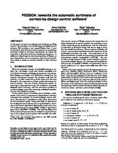
Fig. 3. The variation in peak induced emf measured with each oscillation is shown for initial displacements (θm) (a) 5o, (b) 30o, (c) 55o and (d) 65o
We require the ADC to start the conversion process (analog to digital) as soon as the peak value is attained by the capacitor. This implies synchronization between the input emf pulses and the ADC’s start of conversion (SOC) pulses. To achieve this synchronization it is best to generate the required SOC pulse by wave-shaping the input itself. The sequencing and synchronization can be understood from the various waveforms shown in fig 2b. The second circuit to which the amplified input is fed is also a half wave rectifier. After rectification, output (‘i’ of fig 2b) is fed to a comparator, which compares input signal to +1v. This is to avoid spurious/accidental triggering due to noise. The infinite gain of the comparator results in output pulses with sharp edges (waveform ‘iii’ of fig 2b). The widths of these pulses are approximately To/4 (for our pendulum ~390ms). This would be too large to serve as SOC pulses and hence is reduced to a 5 s pulse using a mono-stable timer made with IC555 [8]. The designed circuit digitalizes the analog emf and on completion sends an EOC to the computer or microprocessor kit (in case of a microprocessor this is done through a programmable I/O IC8155 chip, details of which can be found in the book by Goankar [9]), which then reads the eight, bit data and stores it for retrieval. We used this L8
A. Arora et al., J. Phys. Stu. 2, 3 L6 (2008)
circuit with an 8085 microprocessor kit. The program and flowchart used is detailed in our earlier work [10]. Fig 3 displays the experimental data obtained using the circuit. The strong damping in the pendulum is evident. To summarize, the circuit developed in our under-graduate laboratory helped in giving exposure to Faraday’s induction law and possible application. It also enabled us to study the damping effects acting on the pendulum. Considering the rich information obtained using the circuit and the simplicity of the circuit, we believe it can be easily setup and used for routine experiments in undergraduate laboratories. Acknowledgments The financial support of U.G.C (India) in the form of Minor Research Project No.F.61(25)/2007(MRP/SC/NRCB) for this work is gratefully acknowledged. References [1] M. F. Mclnerney, “Computer-aided experiments with the damped harmonic oscillator,” Am. J. Phys., 53, 991-996 (1985). [2] A. R. Ricchiuto and A. Tozzi, “Motion of a harmonic oscillator with sliding and viscous friction,” Am. J. Phys., 50, 176-179 (1982). [3] P. T. Squire, “Pendulum Damping,” Am. J. Phys., 54, 984-991 (1986). [4] A. Singh, Y. N. Mohapatra and S. Kumar, “Electromagnetic induction and damping: Quantitative experiments using a PC interface” Am. J. Phys., 70, 424-427 (2002). [5] L. F. C. Zonetti, A. S. S. Camargo, J. Sartori, D. V. de Sousa and L. A. O. Nunes, “A demonstration of dry and viscous damping of an oscillating pendulum,” Eur. J. Phys., 20, 85-88 (1999). [6] J. C. Simbach and J. Priest, “Another look at a damped physical pendulum,” Am. J. Phys., 73, 10791080 (2005). [7] X. –J. Wang, C. Schmitt and M. Payne, “Oscillation with three damping effects,” Eur. J. Phys., 23, 155-164 (2002). [8] R. A. Gayakwad, “Opamps and Linear Integrated Circuits,” Prentice-Hall India, Delhi (1999). [9] R. S. Gaonkar, “Microprocessor Architecture, Programming and applications with the 8085/8080A,” Wiley Eastern Ltd. Delhi (1986). [10] A. Arora, R. Rawat, S. Kaur and P. Arun, arXiv:physics/0608071.
L9