HELSINKI UNIVERSITY OF TECHNOLOGY Department of Engineering Physics and Mathematics
Heikki Uljas
Performance evaluation of a subscriber database with queuing networks
Master's thesis submitted in partial fulfillment of the requirements for the degree of Master of Science in Technology Espoo, 30.06.2003
Supervisor: Professor Ahti Salo Instructor: M.Sc. Jukka-Petri Sahlberg
HELSINKI UNIVERSITY OF TECHNOLOGY ABSTRACT OF MASTER'S THESIS Department of Engineering Physics and Mathematics Author: Heikki Uljas Department: Department of Engineering Physics and Mathematics Major subject: Systems and Operations Research Minor subject: Software Systems Title: Performance evaluation of a subscriber database with queuing networks Title in Finnish: Jonoverkot tilaajatietokannan suorituskykyanalyysissa Number of pages: 64 Chair: Mat-2 Applied Mathematics Supervisor: Professor Ahti Salo Instructor: M.Sc. Jukka-Petri Sahlberg Abstract: Often, software development attempts to build software that is correct from the functionality point of view before considering other desirable qualities like security, availability and performance. Commonly the performance of the software is determined only using measurement, which is only possible at a late phase of development. Performance modeling provides means to predict the performance of software before it can be measured. Queuing networks are the most commonly used performance models for software. The software studied in this thesis is a subscriber database that serves as a centralized storage of subscriber preferences for other systems in the network. The database has a capacity of several million subscribers and can serve several thousands of read requests per minute. The thesis studies the performance of one of the services of the subscriber database on three different hardware platforms using queuing network models. The model service time parameter values are estimated on one of the platforms using measurement and are then projected to match the other two platforms based on the hardware performance differences. The results obtained from the model are compared to results from measurement. According to the literature queuing network models are suitable for software performance modeling. The results obtained in the thesis confirm this view. Key words: Queuing networks, Software performance models
TEKNILLINEN KORKEAKOULU DIPLOMITYÖN TIIVISTELMÄ Teknillisen fysiikan ja matematiikan osasto Tekijä: Heikki Uljas Osasto: Teknillisen fysiikan ja matematiikan osasto Pääaine: Systeemi- ja operaatiotutkimus Sivuaine: Ohjelmistojärjestelmät Työn nimi: Jonoverkot tilaajatietokannan suorituskykyanalyysissa Title in English: Performance evaluation of a subscriber database with queuing networks Sivumäärä: 64 Professuuri: Mat-2 Sovellettu matematiikka Valvoja: Professori Ahti Salo Ohjaaja: DI Jukka-Petri Sahlberg Tiivistelmä: Ohjelmistonkehityksessä on monesti pyritty ensin rakentamaan toiminnallisesta näkökulmasta oikein toimiva ohjelmisto ennen muiden toivottavien ominaisuuksien kuten tietoturvan, palvelunsaatavuuden tai suorituskyvyn huomioonottamista. Suorituskyky määritellään usein pelkästään mittaamalla, joka on mahdollista vasta ohjelmistokehityksen myöhäisessä vaiheessa. Mallintamisen avulla on mahdollista ennustaa ohjelmiston suorituskyky ennen kuin se on mitattavissa. Jonoverkot ovat yleisimpiä ohjelmiston suorituskyvyn kuvaamiseen käytettyjä malleja. Tässä työssä tutkittava ohjelmisto on tilaajatietokanta, joka toimii muiden verkon järjestelmien keskitettynä tilaajakohtaisten asetusten tallennusjärjestelmänä. Järjestelmään pystytään tallentamaan miljoonia tilaajia ja se kykenee palvelemaan useita tuhansia lukupyyntöjä minuutissa. Työssä tutkitaan yhden ohjelmiston tarjoaman palvelun suorituskykyä kolmella eri laitteistoalustalla jonoverkkomallien avulla. Mallin palveluaikavaadeparametrit estimoidaan ensin yhdellä laitteistolla mittaamalla, minkä jälkeen ne muutetaan vastaamaan kahta muuta laitteistoa vertailemalla eroja laitteistojen suorituskyvyssä. Lopuksi työssä verrataan mallista saatuja tuloksia mittaamalla saatuihin tuloksiin. Alan kirjallisuuden mukaan jonoverkot soveltuvat ohjelmiston suorituskyvyn mallintamiseen. Työstä saadut tulokset vahvistavat tämän näkemyksen. Avainsanat: Jonoverkot, Ohjelmiston suorituskykymallit
Preface: I want to thank my instructor M.Sc. Jukka-Petri Sahlberg and M.Sc. Vesa Kärpijoki for their help and patience. I would also like to thank my supervisor Professor Ahti Salo for good advice and support. Espoo, 30th of June 2003 Heikki Uljas
4
Table of contents: 1
INTRODUCTION
7
2
SOFTWARE PERFORMANCE EVALUATION
9
3
2.1
Software performance engineering
10
2.2
Limits to performance
12
2.3
Evaluation techniques
14
2.3.1
Measurement
15
2.3.2
Simulation
16
2.3.3
Analytical modeling
17
QUEUING NETWORK MODELS 3.1 3.1.1
3.2
21
Network of centers
21
Types of service centers
3.2.2
Types of workload
24
3.2.3
Product form networks
24
23
Stochastic analysis
26
3.3.1
M/M/1 queue
26
3.3.2
M/M/m queue
27
3.4
Operational analysis
28
3.4.1
Basic quantities
28
3.4.2
Utilization law
29
3.4.3
Interactive response time law
29
3.4.4
Job flow analysis
30
3.4.5
General response time law
31
3.5
Comparison of operational analysis and stochastic analysis
SOLUTION TECHNIQUES FOR QUEUING NETWORK MODELS
32
33
4.1
Bounding techniques
34
4.2
MVA Algorithm
35
4.2.1
Single class MVA
35
4.3
Hierarchical decomposition
38
4.4
Software performance modeling
39
4.4.1 4.4.2
4.5 4.5.1
5
19
Little’s law
3.2.1
3.3
4
Single service center queue
19
SPE execution models Method of surrogates
Sensitivity analysis Uncertainties in model input
PERFORMANCE EVALUATION OF A SUBSCRIBER DATABASE
40 42
43 44
46 5
5.1
Technical description
46
5.2
Shortcomings in earlier performance
47
5.3
Performance modeling
48
5.3.1
Service center identification
50
5.3.2
Workload definition
50
5.3.3
Service time estimation
51
5.3.4
Service time transformation
53
5.4
56
5.4.1
Production hardware A
56
5.4.2
Production hardware B
58
5.5
6
Results
Summary of the results
CONCLUSIONS
REFERENCES:
61
64 66
6
1 Introduction
Traditionally, software development is a functionality-centered process. It attempts to build software that gives correct results before considering other desirable qualities of software like security, availability and performance. The difficulty with performance often is that it is not specified until at the late stage of development when the performance is measured. Performance modeling provides means to predict the performance of software before it can be measured. When used in combination with other techniques like prototyping, it can reduce the performance-related risks in software development. The problem with modeling is that it is not usually part of the software development process and people developing the software are not familiar with modeling techniques or the theory behind them. Also it is not clear what kind of effort the modeling requires and how well the performance of modern software can be described with modeling. Performance models are usually divided in analytical and simulation models according to the applicable solution techniques. Queuing network models are the most commonly used analytical performance models for computer systems and software. The basic principle in queuing network models is that when a resource is reserved by one customer, other customers have to wait for it in a queue. A comprehensive theory and a wide selection of solution techniques exist for the queuing networks [7]. The software studied in this thesis is a subscriber database that is a centralized storage of subscriber preferences for other systems in the network. The software has a distributed architecture for scalability and fault-tolerance. The database itself has capacity of several million subscribers and the system can serve several thousands of read requests per minute. The software is available on several different hardware configurations.
7
The goal of the thesis is to study the feasibility of queuing network models in the performance evaluation of the subscriber database product. The scope of the thesis is limited to a single service of the subscriber database. This is a subscriber preferences read service dedicated to a specific client, which has high performance requirements for throughput and response time. The model is built to determine the performance under similar, artificial conditions the performance tests do. That is, the load for the system is generated artificially and the data content of the database is artificially generated. The thesis starts with a description of software performance evaluation in Chapter 2. Chapter 3 provides a general description of queuing network models and elementary results from queuing theory. Chapter 4 concentrates on describing different solution techniques for solving the queuing network models. Chapter 5 describes the performance evaluation of the subscriber database and Chapter 6 contains the conclusions.
8
2 Software performance evaluation
Traditional software engineering methods have taken the so-called fix-it-later [23] approach towards performance. In this approach the focus is on the functional requirements of the system. The non-functional requirements, such as the security, availability, reliability and performance are typically taken into consideration at the later phase of the development process, i.e. integration and testing [13]. If performance problems are discovered at this point, the software is tuned to correct them or additional hardware is used. It is clear that the fix-it-later approach is undesirable. Performance problems may be so severe that they require extensive changes to the system. These changes will increase the development cost, delay deployment or affect other desirable qualities of a design, such as understandability, maintainability or reusability [23]. Some common reasons for performance problems in software development are [13]: •
Lack of scientific principles and models. Conventional engineers use scientific principles and models based on mathematics, physics and computational science to support their design process. Software engineers do not need to rely on formal and quantitative models; they can write code without formal methods.
•
Education. Topics of computer performance evaluation are not taught to the graduates of computer science.
•
Single-user mindset. Most system designers and programmers who develop systems do not realize that the code they are writing will be instantiated by many concurrent requests.
•
Small database mindset. Code that accesses the database is usually written without taking into account the size of the database. 9
2.1 Software performance engineering The traditional phases of software development process are the following: •
Project planning. The requirements for the software, resource allocation and scheduling are defined.
•
Design. Detailed design that describes how the requirements are implemented is constructed.
•
Implementation. Implementation is done according to design.
•
Testing. It is verified that the software satisfies the requirements.
•
Introduction. The software is deployed into the real environment.
Software performance engineering (SPE) was developed to aid in designing software systems that meet performance requirements [24]. It attempts to estimate the performance at design phase with performance models and to compare design alternatives. The additional activities introduced by the SPE for the software development process phases are: •
Project planning. Tasks required by the SPE are included in the project plan. Potential performance risks are identified and the cost of SPE tasks is estimated [21]. Based on the risk assessment, it is determined how much effort will be put into SPE activities [24]. Performance requirements are defined as part of the software requirements. Resource requirements for hardware, network architecture and software services are specified [21]. Performance critical use-cases are identified; those that are important to performance or those for which there is a performance risk [24].
•
Design. On the basis of performance requirements to the system, the initial performance model is established for each scenario using estimated values. This model is used to check the proposed rough architecture and identify potential
10
performance bottlenecks [21]. Alternatives are compared using a crude model. Refined requirements to be used in design are derived from the model [21]. Benchmarks are used to measure the performance of required services (hardware, middleware, security). With more detailed design the model used is detailed further. The more detailed information can be obtained from measurements of existing systems, benchmarks, manufacturer’s information and estimates. The performance-critical sections of the system are prepared for instrumentation in the design level. More detailed performance requirements are derived for implementation purposes. [21] The performance model is used when considering various design alternatives [24]. If the determined performance is not satisfactory, means of performance improvement considering also other aspects are investigated. These means include changing the design, increasing the planned resource requirement – increasing the overall cost, defining stricter development requirements and reducing the technical demands [21]. •
Implementation. The assumptions established for each model during the analysis and design are replaced with the latest performance data during the implementation [21]. This data is kept up-to-date during the implementation and development of the actual performance is monitored [24]. Instrumentation is inserted to the performance-critical sections of the system.
•
Testing. System performance is tested under conditions resembling the anticipated conditions as closely as possible. The performance models are checked for validity using the performance test data. Possible performance anomalies, i.e. unexpected performance data or behavior are identified. [21]
•
Introduction. The performance behavior of the information system is reviewed in pilot installations over a longer period under real operational conditions [21]. Performance data from the real environment is collected to provide feedback for the development information flow [21]. Model is used to estimate performance effects of changes in the system [24].
11
The activities from above list are illustrated in Figure 2.1. The activities shown are risk management, requirement analysis, performance modeling and performance measurement. Project planning
Design
Implementation
Testing
Introduction
Risk management Project level risks
Identification of critical scenarios
Risk control
Requirement analysis Definition of performance requirements
Refining performance requirements
Verification
Redefinition based on feedback
Performance modeling Comparison of design alternatives
Performance prediction
Model validation
Capasity planning
Measurement Benchmarking services
Benchmarking code
Performance measurement
Data collection
Figure 2.1. SPE activities in software development.
2.2 Limits to performance The performance in computer systems depends on executing elements that reserve and compete on the system resources. The performance is most commonly measured with time, i.e., the time it takes for the system to complete a task, response time or the number of operations performed within time interval, throughput [7]. The resource utilization is also often used as a performance measure [7], like the amount of memory used by the application or amount of disk I/O.
12
In modern computer systems the elements of execution are divided into processes or lightweight processes called threads [26]. They perform tasks for applications or human users utilizing the resources in the system. The performance in a computer system is limited by the service time and resource contention. Service time is the time required for completing a task. All hardware devices in computer systems have physical boundaries that limit the amount of work they can perform per time unit. For example the speed of a processor is governed by its clock rate and instruction length and hard disks are limited by the rotational speed and density of the disk. In early computer systems the operating systems allowed the applications or processes to execute sequentially [26]. When a process started execution it had control over all resources in the system until it was finished. There was always only one active process executing in the system, while all others waited for their turn. Systems with such behavior were called simple batch systems [26] and their performance was limited by the performance of the hardware. The problem with simple batch systems was that since the I/O devices were slow compared with the processor, the processor was often idle. In a multiprogramming system there are many concurrently active processes. When a process begins to wait for I/O, it is switched out from the processor and another application is switched in. [26] From the performance point of view, multiprogramming means two things: •
The overall performance of the system is improved since processes can use different resources independently.
•
The performance of an individual process may become worse because of resource contention.
Resource contention is caused by competition on hardware resources. When a resource is reserved by one process, other processes have to wait for it to become free. In such a case, performance is determined by a combination of wait time and service time. The gain in performance from resource sharing is generally more than the loss due to resource contention. [26] 13
Hardware devices such as processor or disk are usually limited by both service time and resource contention. Executing processes wait for the device, use it for service and release it for others to use. The reservation of these devices is handled by the operating system. Devices that have high capacity compared to their load do not necessary have resource contention, but do have service time. Some resources may be delay type, like with users accessing the system through a user interface. A user executes some operation and then spends some time looking at the results. This time is in general called the think time [7]. Some resources are required for processing but they do not perform any work. Memory is an example of such resource where the limiting factor is the resource contention alone. Critical software resources such as locks or semaphores used in synchronization [26] fall also into this category. These three different types of resources are listed in Table 2.1. Table 2.1. Different types of resources in computer systems.
Resource type
Service time
Service time with limited Limited. capacity. Service time with infinite Limited. capacity. No service time with None. limited capacity.
Resource contention Limited.
Examples
None.
Network delay, human users. Memory, software resources.
Limited.
CPU and disk.
2.3 Evaluation techniques The most common technique used in performance evaluation is measurement. Every system where the performance is important the performance is at least measured. A more rarely used way is modeling. Two types of models are used, analytical and simulation models, depending on the solution method used. These two modeling techniques can also be combined to through hybrid modeling [7] [9]. What technique is used depends on the development stage of the system, required accuracy of results and resources available for the evaluation. Any of these techniques might give results that are misleading or wrong [7]. It is not stated that performance evaluation 14
is done using only one of the technique, different sections in a study might be solved using different techniques. For example, the system could be divided into sub-systems and the performance for each sub-system might be determined using different techniques. The total performance could then be determined using either simulation or analytical model. Another example is the use of measurement in the parameterization of models.
2.3.1 Measurement Measurement is the most fundamental technique for performance evaluation. It is commonly used to verify that a system meets its performance requirements. It is used with analytical and simulation modeling to obtain parameter values for the models and to validate the results. In a normal situation there is a system with a specific configuration and workload running on that system. In addition to that the measurement is affected by random fluctuation. [1] When conducting a measurement, it is important to collect data for all four quantities shown in Figure 2.2. Careful tracking of configuration changes and monitoring of the workload levels is required. The random noise can be handled using statistical analysis of results. [1]
System configuration
Workload applied to the system
Computer system for measurement
Performance measurements
Random fluctuation
Figure 2.2. Conceptual model of system under measurement.
The measurement technique is the most accurate of the techniques if the premises are correct and the measurement is conducted appropriately. It is commonly used and therefore credible. Measurement requires some time for preparing the test, collecting the data 15
and analyzing the results. On the other hand, it is prone for disruptions and can be very time consuming if there are unexpected difficulties. The most serious drawbacks of measurement are that it may be very expensive and requires a functioning system [7],[20]. These problems can be addressed with prototyping but this usually requires some kind of model for uncertainty analysis and estimation of the total performance of the system since only part of the functionality is covered by the prototype. Another drawback is that measurement technique is likely to give accurate knowledge of system behavior under one set of assumptions, but not any insight that would allow generalization [11].
2.3.2 Simulation The simulation technique involves the construction of a simulation model of the system’s behavior and running it with an appropriate abstraction of the workload. It is used when analytical modeling is infeasible. It might be difficult to construct an analytical model of the system or the model could be impossible to solve by analytical means. The major advantage of the simulation is that almost any kind of behavior can be simulated. [9] The parameters that correspond to the workload and configuration of the actual system are given for the simulation model as input. The model is evaluated repeatedly and random variables are used in every evaluation round. Simulation data is received as a result, which is then analyzed to get performance measures. These concepts are illustrated in Figure 2.3.
16
System configuration parameters
Workload parameters
System under study
Simulation data
Generated random noise
Figure 2.3. Conceptual model of system for simulation.
Simulation models are more comprehensive than analytical models in the sense that more details can be included in them. If the model is sufficient, it will provide accurate results. The building of a simulation model may require a long time if no ready simulation software is available. Simulation does not depend on the development stage of the system, so it can be used for example in the design phase. [7]
2.3.3 Analytical modeling Analytical modeling involves the construction of a mathematical model of the system behavior after which the model is solved analytically. The problem with this approach is that the domain of models solvable by analytical means is limited. Thus, analytical modeling will fail if it is required to study the system in great detail. Simulation can be used to solve more detailed models. [9] Analytical models are parameterized to describe the workload and system configuration. Sensitivity analysis is used to determine the sensitivity of the performance estimates to the model parameters [22]. The estimates with their confidence intervals are received as results from the model. These concepts are illustrated in Figure 2.4.
17
System configuration parameters
Workload parameters
Analytical model
Estimates of performance
Confidence analysis
Figure 2.4. Conceptual model of a system for analytical modelling.
Analytical models tend to be less accurate than simulation models in that very complex models cannot be solved by analytical means. However analytical modeling is usually the cheapest and fastest of the techniques [7] and it can also be used with incomplete systems [20]. Analytical modeling can provide valuable insight into the functioning of the system even if the results are not correct [11], since the system has to be understood before the model can be built. Very abstract and simple models can provide surprisingly accurate estimates of the system performance and results from the analysis have better predictive value than those obtained from measurement or simulation [9]. Commonly used analytical models are queuing network models [13], [2]. More simple models can also be used, such as the software execution model [24].
18
3 Queuing network models
This chapter describes the basics of the queuing network models in that extent they are used in the later sections of this thesis. The main focus is on simple results that can be easily adopted in software performance evaluation. Sophisticated stochastical analysis is not in the scope of this thesis. In a queuing network model the system is represented as a network of service centers, which represent system resources, and customers, which represent users or requests. Queuing networks are used because their structure closely resembles the structure of computer systems. Operating systems for example use queue-like structures, which are used to handle resource contention. Queuing network models have been widely used in computer system performance modeling. Experience indicates that queuing network models can be expected to be accurate to within 5% to 10% for utilization and throughput and to within 10% to 30% for response times [11].
3.1 Single service center queue In its simplest form, a queuing network consists of a single service center. Customers arrive at the center, wait their turn in the queue if necessary and depart. This simple queue is illustrated in Figure 3.1.
19
Queue
Server
Arriving customers
Departing customers
Figure 3.1. Single service center queue.
The basic quantities used to describe a center are: •
Arrival rate (λ): Describes the number of arrivals to the center in unit time. Expressed in requests per second or jobs per second (req/s or jobs/s).
•
Service time (S): The amount of time the customer spends in the service. Expressed in seconds or milliseconds (s or ms).
•
Number of devices (m): The number of devices serving the requests for the center.
Basic performance measures obtained from a center are: •
Utilization (U): The utilization can be understood as the fraction of time the center has a customer or is busy. For a center with multiple devices this definition does not take into account the number of devices that are reserved. An alternative definition of the number of customers in service is more accurate in such a case. Utilization is expressed as percentage, where 100% means a fully utilized service center in a single device case. The maximum utilization for a multiple device center is m*100%.
•
Throughput (X): Describes the number of departures from the service center per time unit. Used units are requests per second or jobs per second (req/s or jobs/s).
•
Response time (R): The time the customer spends in the center, including the wait and service times. Usually expressed in seconds or milliseconds (s or ms).
20
•
Queue length (Q): The number of customers in the center, including both the customers waiting for service and receiving it.
3.1.1 Little’s law The following relationship is known as the Little's law and it was first proved in [12]. It states that N = λR
3-1
where N is the average number of customers in the system, λ is the arrival rate to the system and R is the average time spent in the system. Little's law holds for all those systems where the number of arrivals equals the number of departures. It is important because it can be used with most queuing systems and applies to both single center systems and network of centers as well.
3.2 Network of centers In a network of centers multiple centers are connected with each other. Requests flow through the system receiving service on different service centers. When a customer departs from a center he proceeds to another until his service requirements have been met. In an open network, like the one shown in Figure 3.2, customer population for the system is infinite and customers arrive and depart from the system freely. The number of customers in the system varies over time.
21
Arrivals
Departures
Figure 3.2. Open queuing network.
In a closed network the customer population is fixed so the customers never leave or arrive at the system. Figure 3.3 shows an example of a closed network. Closed networks are used to model systems, which have some constraints on the number of customers. However open networks are easier to analyze than closed ones.
Arrivals
Departures
Figure 3.3. Closed queuing network with its open subnetwork.
The basic quantities used with queuing networks are: •
Arrival rate (λk): Describes the number of arrivals to the kth center in unit time. Used to describe the workload in open networks.
•
Routing probability (pkl): The probability of a customer departing from the kth center to proceed to the center l.
•
Service time (Sk): The amount of time customer spends in service in center k.
•
Number of devices (mk): The number of devices serving the requests for the kth center.
•
Number of centers (K): The number of centers in the network
•
Number of customers in the network (N): The sum of all customers in all centers of the network. Fixed in a closed network. 22
•
Think time (Z): The time that the customer spends thinking between visits to the system. Used when modeling interactive systems.
Basic performance measures obtained from a center are: •
Center utilization (Uk): The utilization for center k.
•
System throughput (X): The throughput of the whole network.
•
Center throughput (Xk): The throughput of the kth center.
•
System response time (R): The response time of the whole network.
•
Center response time (Rk): The response time of the kth center.
•
Queue length (Qk): The number of customers in the kth queue.
The units used with a network are the same ones used with a single service center.
3.2.1 Types of service centers There can be different kinds of service centers in a queuing network. Here they are divided into load-independent, load-dependent and infinite service centers due to the difference in the analysis they require. In a load-independent service center the service rate of the service center is independent of the number of customers in the center. An example of this kind of a service center is a subsystem with single device serving the requests, such as a single processor. Load-dependent and infinite service centers are examples of service centers where the service rate depends on the number customers in the service center. Load-dependent center can be used to model any kind of load-dependent behavior. Commonly loaddependent centers are used for subsystems where multiple devices serve a single queue, but are also used when a single device or subsystem has load-dependent behavior. The infinite service center is a special case of load-dependent service center where the customer never waits for service. In it the number of devices serving the customers is always larger than the number of customers at the center. Infinite service centers are also 23
sometimes referred to as delay centers. Infinite service centers are used to model resources that have infinite capacity with some service time.
3.2.2 Types of workload The workloads for a system can be divided into transaction, batch and interactive workload [11]. In transaction workload the customers arrive and depart the system freely. Therefore an open network is used for modeling it. The workload intensity is defined by the rate of arrivals to the system. In batch workload the number of customers in the system remains constant. In interactive workload the number of customers in the system does change due to the time they spend thinking between the operations. The batch workload can be thought of as a special case of the interactive workload where the think time is zero. Closed networks are used to model systems with batch or interactive workload and interactive workload is modeled with open network. The workload intensity in interactive workload in defined by the number of customers in the system and think time. The think time in interactive workload is included in the model as an infinite service center, as shown in Figure 2.2.
Figure 3.4. Network with interactive workload.
3.2.3 Product form networks A major difficulty in the analysis of network of queues is that the state of a single queue may depend on the state of other queues. Fortunately a large subset of queuing networks called the product form networks [7] allows the analysis of the queues to be done separately.
24
Product form networks have the property that the measures of performance, such as mean queue length or response times are insensitive to the higher moments of distributions of service times, and depend only on the mean service time. Furthermore, they do not depend on the order in which the service centers are visited nor on the number of times a service center is visited but only on the total demand that a customer places on a service center. [19] A network is a product form network if it has the following properties: •
The interarrival-time distribution is exponential for open network. [9]
•
Each center in the network is one of the following three types: 1. Delay center with general service-time distribution for each class. [9] 2. FCFS (First-Come-First-Served) center with the same exponential service time for each class. The center may be load-dependent, but the service rate may only be dependent on the total customers at the center. [7] 3. PS (Processor-Sharing) center with arbitrary service-time distribution for each class. The station may be load-dependent, with some restrictions on the load dependency among different classes. [9]
•
For each class, the number of arrivals to a center must equal the number of departures from the center. [7]
•
A customer may not be present at two or more centers at the same time. [7]
The FCFS and PS are examples of queuing disciplines. A queuing discipline describes the order in which the customers are served at the center. With FCFS, the customer that arrives at the center first is served first. With PS, the center is shared by the customers and they all receive service at the same time. [7] The list presented above is not complete, a more complete listing can be found at [7] or [9]. The exact mathematical representation of product form networks can be found at [14].
25
3.3 Stochastic analysis In the traditional stochastic analysis of queuing networks the queues are modeled as random processes, whose state is defined by the number of customers in them. A random process describes the probabilities of the states of the system over time. Service times and the times between arrivals are modeled as random variables with known probability distributions. A shorthand notation of form A/S/m is used to describe a single queue, where the letters stand for arrival process, service time distribution and number of devices in the queue [14]. An important and widely used probability distribution is the exponential distribution [5], which is denoted with the letter M. The letter M refers to the memoryless property that the distribution has [14]. For a service time the memoryless means that the remaining service time does not depend on the time the customer has already spent in the service.
3.3.1 M/M/1 queue The simplest possible queue is the M/M/1 queue. It is a single-device queue with Poisson arrivals and exponential service times. This queue is an example of a loadindependent center. The customers arrive and depart from the M/M/1 queue one at a time. The state transition diagram shown in Figure 3.5 can be used to illustrate the transitions between different states. λ
λ 0
λ i-1
1 µ
λ
µ
µ
λ i
µ
λ i+1
µ
µ
Figure 3.5. State transition diagram for M/M/1 queue.
Since there is only one customer arriving or leaving the system, the transitions in the system occur only between adjacent states. And since the arrival of a new customer is inde26
pendent from the systems state, the arrival rate λ is same for every state. Furthermore, since the completion of a customer is independent from the systems state, the service rate µ is the same for every state. The service rate of the M/M/1 center is [14]:
µ=
1 S
3-2
where S is the average service time of a customer. The probability of having n customers in the center is [14]: p (n ) = (1 − ρ )ρ n where the term ρ =
3-3
λ is called traffic intensity. µ
The utilization of the service center is given by the probability of having more than 0 customers in the system. From (3-3) we get U = 1 − p0 = ρ
3-4
The average queue length is given by [14]:
Q=
U ρ = 1− ρ 1−U
3-5
Using Little's law from (3-1) with (3-5), the average response time for the queue is
R=
1/ µ S = 1− ρ 1−U
3-6
3.3.2 M/M/m queue Commonly required extension to the M/M/1 queue is a variant with m identical devices serving the requests. This kind of a queue is called the M/M/m queue. It is an example 27
of load-dependent center where its service rate of the center µ depends on the number of customers in the center n. The service rate of the center is [7]:
ì n ⋅ µ0 µ (n ) = í îm ⋅ µ 0 where the µ 0 =
n
3-7
1 denotes for the service rate with only single customer at service. FurS
ther results for the M/M/m queue can be found at [7].
3.4 Operational analysis Operational analysis is based on assumptions that can be verified by observing the system over a finite time interval [3]. Average values are used for the service time and arrival rate. Many of the operational results are identical to those obtained with stochastic analysis, but have the advantage of being more intuitive and applicable to nonstochastic systems as well [9].
3.4.1 Basic quantities Suppose that a single center system shown in Figure 3.6 is observed for a finite time period T. During this number of arrivals to A, number of completions from C, and the busy time B for the system are collected. [3]
28
A
D B
Figure 3.6. Simple system.
Using these definitions we can derive some basic quantities from section 3.1:
λ = A/T
3-8
X = C /T
3-9
U = B /T
3-10
S = B/C
3-11
Where S is the average service time of the center. [3]
3.4.2 Utilization law Using (3-9), (3-10) and (3-11) we can derive a relationship known as the utilization law [3]:
U=
B C B = ⋅ = X ⋅S T T C
3-12
The utilization law binds the utilization of a resource together with its throughput using the average service time. The utilization law is a special case of the Little's law from (3-1) when the system is observed without the queue.
3.4.3 Interactive response time law In an interactive system, like the one shown in Figure 3.4, N users generate requests that are served by the system. The user spends think time Z thinking before he submits the 29
next request. If the average response time is R , the total time a user spends in the waitthink cycle is R + Z. Throughput X denotes the rate at which cycles are completed. Little's law from (3-1) leads to
(
N = X R+Z
)
3-13
which then leads to
R=
N −Z X
3-14
This relation is known as the interactive response time law. [3]
3.4.4 Job flow analysis If the observation period is long enough so that difference between arrivals and completions Ak − C k on each device k is small compared to C k , it can be assumed that the relation Ak = C k holds. This assumption is called the job flow balance assumption because it implies that λk = X k for each device k. When the job flow is balanced, we refer to the
X k as center throughputs. The visit ratio Vk , which expresses the average number of visits on device k for customer, is derived as:
Vk =
X k Ck = X C
3-15
Where X and C are the throughput and completion count from the whole system. Using the visit ratio we can define relation called the forced flow law:
X k = X ⋅ Vk
3-16
30
It applies whenever the job flow balance assumption holds. The forced flow law states that various devices in the system must do comparable amounts of work in a given time interval. Service time and visit ratio for a device together determine the amount of service a job requires from a service center. Therefore they are usually replaced with the total service time of center k [7]:
Dk = Vk S k
3-17
3.4.5 General response time law With the Little's law from (3-1), and if the job flow balance holds, the average response time of the system can be expressed as
R=N/X
3-18
If the N or X are not known an alternative method is to use visit ratios. Applying the Little's law from (3-1) to device k and using the forced flow law from (3-16) results
Qk / X = Vk ⋅ Rk which with
3-19
3-18) leads to K
R = å Vk Rk
3-20
i =1
This equation is called the general response time law [3].
31
3.5 Comparison of operational analysis and stochastic analysis The operational analysis offers more intuitive and simple proofs to several results that would be difficult to obtain stochastically. The results obtained from the operational analysis are easier to explain to a person with no earlier experience on probability theory. Under comparable assumptions, many of the results obtained from these two approaches are identical. With operational analysis the defined properties depend directly on the given behavior sequence. Thus, average really means sample average and probability really means relative frequency. [9] Probability distributions used to describe variables and results in stochastic analysis are replaced with average values in operational analysis. Since randomness is not included in the operational analysis, the variability of the results has to be analyzed separately. Although the operational analysis makes it convenient and easy to understand relations for the quantities in the queuing system, it cannot answer questions that require knowledge about the stochastic process underlying in the system. For example solving response time and queue length of a queuing center requires additional assumptions about the distributional properties of the service time. The problem with stochastic analysis is that distributional properties of the random variables are hard to obtain and the assumptions are difficult to prove.
32
4 Solution techniques for queuing network models
This section presents different solution techniques for some queuing networks. Customers in the networks are divided into classes where each class has its own workload parameters and service time requirements. Based on the number of classes the networks can be further divided into single and multiple class networks. The single class model is appropriate choice if:
•
The computer system under consideration has only a single workload of significance to its performance.
•
The various workload components of a computer system have similar service demands.
Conversely, there are number of situations in which it might be inappropriate to model a computer system workload by a single customer class. The multiple classes are then used instead. Such situations are [11]:
•
The workload components on the system are so different that a single class representing an average customer might not provide accurate results.
•
The use of the model requires class-dependent input parameters.
•
The use of the model requires class-dependent output parameters.
The solution techniques introduced in this section rely on the queuing network analysis described in the previous section. They can all be used for all those networks that satisfy the product form network assumptions presented in Section 3.2.3.
33
4.1 Bounding techniques Asymptotic bounds provide simple limitations for the system response time and throughput. They are applicable under very general assumptions. These bounds are based on the fact that the utilization of a load independent service center cannot exceed 100%. The format of the bounds is the following:
ì 1 N ü X ≤ min í , ý î Db D + Z þ
{
R ≥ max D, N ⋅ Db − Z
4-1
}
4-2
The subscript b refers to the bottleneck device, the device with the largest total service time. [3] Although the asymptotic bounds provide bounds under very general conditions, they are only one-sided. Two-sided bounds called the balanced bounds are based on the observation that a balanced system has a better performance than a similar unbalanced system [27]. A balanced system is a system where the service times on every service center are equal. The balanced bounds have the following format [27]:
(
N
)
D + N − 1 Db
≤X≤
N D + ( N − 1) Davg
D + ( N − 1) Davg ≤ R ≤ D + ( N − 1) Db
4-3
4-4
where Davg corresponds to the average total service demand per service center, which is D/K.
34
4.2 MVA Algorithm Mean-Value Analysis algorithm is used for solving closed queuing networks. It is a recursive algorithm where the solutions from the previous iteration are used as basis of the next iteration. The MVA starts from an empty system and continues increasing the number of customers in the system on every round. On each round the following steps are executed [11]: 1. Calculate the response time on every center based on the service rate and queue length distribution of the center seen by an arriving customer. 2. Calculate the total throughput of the system using the response time. 3. Calculate the queue length distribution for current population using the throughput. The exact MVA algorithm is very complex algorithm with large networks and customer populations. Because of this, approximative algorithms have been developed that reduce the computation effort required by the MVA algorithm. These algorithms use different approximations to calculate the response times on step 1. The algorithm explained in this section is the exact MVA algorithm. Most approximative MVA algorithms can be found at [15].
4.2.1 Single class MVA The MVA does have simpler form for load-independent and infinite servers, but since those results can be derived from the general, load-dependent form that is presented here first. Let µ k ( j ) be the service rate of the kth center when there j customers there. Let
p k ( j | n ) be the probability of having j customers at the center k when there are n customers in the system. Then the average response time of the kth center is [11]:
35
n
Rk (n ) = å j =1
j
µk ( j)
⋅ p k ( j − 1 | n − 1)
4-5
With the response time it is possible to calculate the system response time using the general response time law from (3-20). The system throughput can be then calculated with the following equation [11]:
X (n ) =
n Z + R (n )
4-6
The system throughput is then used to update the queue length probabilities with the following equation [11]: X (n ) ì ïïVk ⋅ µ ( j ) ⋅ p k ( j − 1 | n − 1) k pk ( j | n) = í n ï 1 − å p k (i | n ) ïî i =1
j = 1,..., n
4-7 j=0
It is sometimes convenient to express the service rate by the service rate a single customer would finish the service. This is done using service rate multipliers α k ( j ) which are defined to be:
α k ( j) =
µk ( j) = Sk ⋅ µk ( j) µ k (1)
4-8
where S k is the average service time of center k with only one customer in it. Using this result (4-5) becomes: n
Rk (n ) = S k ⋅ å j =1
j
α k ( j)
⋅ p k ( j − 1 | n − 1)
4-9
and (4-7) becomes: X (n ) ì ïï S k ⋅ Vk ⋅ α ( j ) ⋅ p k ( j − 1 | n − 1) k pk ( j | n) = í n ï 1 − å p k (i | n ) ïî i =1
j = 1,..., n
4-10 j=0
36
Using the forced flow law from (3-16) with the utilization law from (3-12) this becomes: ìU k (n) ïï α ( j ) ⋅ p k ( j − 1 | n − 1) ( ) pk j | n = í k n ï 1 − å p k (i | n ) ïî i =1
j = 1,..., n
4-11 j=0
where U k (n) is the utilization of the device k when there are n customers at the system. The response times shown in the algorithm for both load-dependent and infinite center can be derived from the equation shown above. For load-independent center the service rate multiplier is one, as shown in (3-2). This leads to: n
Rk (n ) = S k ⋅ å j =1
j
α k ( j)
n
⋅ p k ( j − 1 | n − 1) = S k ⋅ å j ⋅ p k ( j − 1 | n − 1) j =1
n −1 æ ö = S k ⋅ çç1 + å j ⋅ p k ( j | n )÷÷ = S k ⋅ (1 + Qk (n − 1)) j =1 è ø
where the definition of mean x = å xi ⋅ p ( xi ) [10] has been used. i
For infinite server the service rate multiplier is the number of customer at the center, j. When this is used with (4-9) the result is: n
Rk (n ) = S k ⋅ å j =1
j
α k ( j)
n
⋅ p k ( j − 1 | n − 1) = S k ⋅ å j =1
j ⋅ p k ( j − 1 | n − 1) j
n
= S k ⋅ å p k ( j − 1 | n − 1) = S k j =1
since the probabilities p k ( j − 1 | n − 1) sum up to 1. For a center with m identical devices the service rate multiplier is: ì j j
4-12
For such center (4-9) gives:
37
n
Rk (n ) = S k ⋅ å j =1
j
α k ( j)
⋅ p k ( j − 1 | n − 1)
n ù ém j j = S k ⋅ êå ⋅ p k ( j − 1 | n − 1) + å ⋅ p k ( j − 1 | n − 1)ú j =m m û ë j =1 j m n é ù j = S k ⋅ êå p k ( j − 1 | n − 1) + å ⋅ p k ( j − 1 | n − 1)ú j =m m ë j =1 û
4.3 Hierarchical decomposition The hierarchical decomposition technique simplifies the analysis of complex queuing networks. The network is simplified by replacing part of the network, called the aggregate subnetwork, with a flow-equivalent center (FEC). This allows the analysis of the rest of the network, called the designated subnetwork to be done in isolation. The hierarchical decomposition is summarized with the following steps [7]: 1. Select the designated subnetwork. The remaining queues belong to the aggregate network. 2. Create a shorted model by setting the service times of all centers in the designated subnetwork to zero. 3. Solve the shorted model. 4. Create a equivalent model by replacing the aggregate network by an FEC. The flow-equivalent center is a load-dependent center whose service rate is equal to the throughput of the shorted model with all n. 5. Solve the equivalent network. The performance measures for service centers in the designated subnetwork, as obtained from the equivalent network, apply to the original network as well. The hierarchical decomposition can be used for hierarchical modeling. In a hierarchical model the system is modeled in layers where each layer contains more details than the
38
previous layer. The model is solved starting from the most detailed layer and representing it as a FEC in the next layer. An example of model decomposition is shown in Figure 4.1.
Disk subsystem
CPU subsystem
Disk controller CPU CPU
Disk Disk Disk Figure 4.1. Example of model decomposition.
4.4 Software performance modeling The models used to model software performance are based on the queuing network models explained earlier in Chapter 3. However, the complexity of software is often a problem.
39
Software has a large number of operations, like method calls of which most have no significant effect on performance. Important sections are often hidden under structure of abstractions, parallelism or external libraries. Modeling the software using its total service time is not desirable because it offers no insight in the working of the software and offers little insight in the performance under different circumstances. A better alternative is to use a detailed model that describes the software execution with resource service time estimates. This kind of a model is a natural choice when the system is under development since the software consists of smaller pieces of execution for which the performance is estimated separately using different approaches. Also different input may cause different execution and therefore different performance. Sometimes software itself has structures that can be considered as resources. These include single-thread server objects, critical code sections and database locking mechanisms. From the modeling point-of-view these resources have limited capacity but no service time. Together with hardware resources the system has simultaneous resource possession, which cannot be modeled using traditional queuing network models. Extended queuing network models exist that can be used to model simultaneous resource possession.
4.4.1 SPE execution models In SPE [24] it was suggested to use two kinds of models for software performance modeling: 1. Software execution model is used to describe the software execution and to obtain hardware resource demands. 2. System execution model is used to describe the system's hardware resources. This approach attempts to simplify the estimation of resource requirements by dividing the software into smaller parts for which the performance is easier to estimate and analyze. The software execution model describes the software execution in a similar manner as the sequence diagrams used in the UML [16]. Figure 4.2 shows examples of these models with performance attributes. The output of the software execution model is
40
transformed to system execution model service times. The system execution model is equivalent with a traditional queuing network model. In the software execution model the execution of the software is described with a graph where each node corresponds to activity with some performance cost associated with it. There are also special nodes that represent repetition, conditional execution or other software structure related concepts. The costs are expressed per software resource. Software resource is a performance unit that can be easily used to describe the software performance. It can for example be single disk operation, remote call or hardware resource requirement on the reference hardware. When the software execution model is complete the model is solved to obtain the total demands per software resource. The software service demands are then transformed to hardware service demands, which are used to parameterize the queuing network model. The queuing network model can then be solved with basic solution techniques.
41
Client
Server
Database
CPU
Disk
getData(id): select(id):
Process request
CPU=1 Disk=0
Select
Handle result
CPU=1 Disk=1
CPU=3 Disk=0
Figure 4.2. Software execution models with performance attributes.
4.4.2 Method of surrogates The method of surrogates is an approach to modeling the simultaneous resource possession of resources in queuing networks. It is applicable in such situations where a customer acquires one resource, referred to as the primary resource, and holds it both for a preliminary service time and while obtaining and using some other resources, referred to as the secondary subsystem. [6] The method of surrogates uses two models. The first model captures the component of overall queuing delay that is ignored by the second model. It has explicit representation of the primary resources and the congestion due to the secondary subsystem is repre-
42
sented with a delay center. The second model has a flow-equivalent center representing the secondary subsystem and a delay server representing the primary resources. [6] The solution is obtained by solving the first model with service time set to zero for the delay server representing the secondary subsystem. From the solution the primary resource queuing delay can be estimated and is then used to parameterize the delay server representing the primary subsystem in the second model. This solution is then used to parameterize the delay server at the first model. The final solution is obtained by iterating between the two models until the difference in waiting time between the solutions becomes negligible. [6]
4.5 Sensitivity analysis Sensitivity analysis is the study of how the variation in the output of a model can be traced to different sources of variation. Most commonly sensitivity analysis deals with uncertainties in the input variables and model parameters, but it can be extended to associate uncertainty in model structures and assumptions. As a whole sensitivity analysis is used to increase the confidence in the model and its predictions, by providing an understanding of how the model outputs respond to changes in the inputs. [22] Models input may be influenced by many sources of uncertainty including:
•
Measurement errors
•
Lack of information
•
Poor understanding of the system
With queuing network models the key input parameters are the workload intensity and center service times.
43
4.5.1 Uncertainties in model input The simplest way to describe uncertainty is to use interval for the parameter value. This uses the extreme values to describe the parameter, minimum and maximum. A problem arises when the two extremes provide a result that is both acceptable and unacceptable. In such situation some additional information would be required for decision making. The benefit of interval approach is that it is simple to conduct the model is just evaluated with the extreme values. A better way to describe the uncertainty of a parameter is to use probability distribution. The model is then executed repeatedly for the parameter values sampled with some probability distribution. The result is a distribution for the model outputs. The problem is the choice of correct distribution; there might not be enough information available to support the selection. For the queuing network parameters, the center service time is obtained from measurement data using the utilization law from (3-12). If the throughput X and utilization U have nominal values of X0 and U0 and the uncertainties are ∆X and ∆U the uncertainty of S can be estimated with [4]:
∂S ∂S U =U 0 , X = X 0 ⋅ ∆U + ∂X ∂U U 1 ≈ ⋅ ∆U + 02 ⋅ ∆X X0 X0
∆S ≈
U =U 0 , X = X 0
⋅ ∆X 4-13
If the throughput X and utilization U have sample averages of X and U and sample variances of σ U2 and σ X2 the variance of service time S can be estimated with: 2
æ ∂S æ ∂S ö σ S2 ≈ ç ⋅ σ U2 + ... + ç U =U , X = X ÷ è ∂X è ∂U ø 2 1 U ≈ 2 ⋅ σ U2 + 4 ⋅ σ X2 X X
2
ö ⋅ σ X2 U =U , X = X i ÷ ø
4-14
The first equation is used for describing uncertainties that are not represented by measurement data like measurement accuracy. The second equation is used to represent the
44
uncertainty caused by random fluctuation in the data. The total uncertainty of the service demand is the combination of those values and can be expressed with:
∆ total S = ∆S + 2 ⋅ σ S
4-15
The factor 2 in the equation stands for 95% confidence interval for normally distributed random variables. The fact that the service time is not necessarily normally distributed is omitted here. When a model is solved for example using the MVA algorithm presented earlier, the uncertainty can be used in describing the extreme values for the service time values. The model can then be solved using those extreme values to determine the uncertainty in the model outputs. For more detailed approach the service time can be sampled using a random distribution and the model can be solved repeatedly to obtain performance measure distributions. If the model service times cannot be measured, for example because the system is not complete, this would naturally affect the uncertainties. With a detailed model service time of some parts of the software can be benchmarked and others can be estimated based on information from earlier versions or other systems. The uncertainties may have to be estimated case by case, resorting mainly on expert's opinion. Probably the only feasible way would be to estimate the service times of each section using intervals and then combine these values to obtain the minimum and maximum total service.
45
5 Performance evaluation of a subscriber database
The subscriber database, henceforth the "system", is a product applied by external clients in the network as a centralized storage of subscriber information. This information includes subscriber preferences used by the external clients in the network. The system has the storage capacity for several million subscribers and can serve tens of thousands read operations per minute. The basic service provided by the subscriber database involves reading of subscriber preferences from the database. The system has also other services like a service for importing subscriber data and a user interface, which can be used by a system administrator to manage the system data or a user to modify his own preferences. This thesis is limited to a subscriber preferences read service for a specific client, which is the most important service provided by the system. This service reads the subscriber's preferences from the database and uses that information to determine the response to the external client’s request. The service has high performance requirements for system throughput and response time.
5.1 Technical description The subscriber database has an Oracle [17] database, which is used for storing the subscriber data. The application layer of the system consists of distributed servers, which provide services to other objects in the system and clients in the network. The implementation of these servers is done in java [8] and they use JDBC [8] to access the database. The goal of the distributed architecture is to provide reliable service and scalability.
46
The client accesses the subscriber database through a front-end component that is dedicated to that particular client. The front-end handles the data conversion between the client and the component containing the actual business logic, the core. The core uses the information in the request to read data from the database. The response for the client’s request is produced from the data read from the database. The core returns the response to the front-end component, which transforms it to the client format and returns it to the client. The system components are shown in Figure 5.1.
Client NodeA ClientA
Subscriber database Front-end
Core Database
Client NodeB ClientB
Front-end
Figure 5.1. Subscriber database components.
5.2 Shortcomings in earlier performance The system had high performance requirements and adequate performance was one of the key criteria for the success of the project. The performance was always considered when making design decisions, but no formal approach was applied. Some middleware alternatives were compared using benchmarks, but the performance of the whole system was not known until it was measured. Based on the experience from earlier versions, certain operations were known to be expensive and it was known how the performance could be improved. What influence the different parts of the software had on the total performance was not known.
47
Initially the subscriber preferences read service, which is studied in this thesis did not did not meet the requirements set for its throughput. Separate performance improvement activities were required before the throughput reached acceptable level. Some changes to the original design were required. These activities did take several weeks to complete and delayed other activities, especially formal testing. After the performance improvement all tests had to be re-executed. The performance improvement was based on experiences from the earlier version of the system. Different changes were tried out and their effects were verified using measurement. The most effective changes were caching part of the data and changing the request and response handling algorithm. Together these two changes increased the throughput by 100%.
5.3 Performance modeling The goal was to build a model of the system that could be used to estimate the systems performance on different hardware platforms. The model structure was based on knowledge on systems performance behavior. The service time values were estimated on the development platform using measurement. Benchmarks were used to compare the hardware speed differences between the CPUs on different platforms. The estimated service time values were transformed for the production hardware model using the results from the CPU speed comparison. The model was then solved and the results were compared with measurement results. The performance modeling of the subscriber database is illustrated in Figure 5.2.
48
Study system
Development hardware
Production hardware
Determine workload
Identify service centers
Measure performance
Run benchmark
Measure performance
Run benchmark
workload type
service centers
dev. performance data
dev. hw speed
prod. performanc e data
prod. hw speed
Estimate service times
Compare hardware speeds
hw speed ratio dev. service time estimates Transform service times prod. service time estimates Solve model
performance estimates
Verify results
Figure 5.2. The performance modeling of subscriber database.
One development and two production hardware configurations were used in the thesis. These hardware configurations are listed in Table 5.1. The performance metrics of interest were system throughput and response time. The maximum throughput was especially important since the performance requirements for it were tight. The requirements for the average response time were less demanding.
49
Table 5.1. Hardware configurations used in the thesis. Hardware
Number of CPUs Relative CPU clock rate
development
1
1
production A
2
1.79
production B
8
1.49
5.3.1 Service center identification From hardware resources it was known that the CPU was the bottleneck device. In performance tests the CPU utilization did increase with the load, while the disk usage remained close to zero. This was because the database memory cache was sufficient to hold the data used in the tests, so no disk access was required. The application components front-end and core both had thread pools, which handled the incoming requests. Since the size of the pools was not limited, they were not considered as a performance problem and were omitted from the model. Similar situation was also with the database connections. These connections were cached in a pool to improve the performance. The size of this pool was limited to twenty connections, but was large enough to handle number of threads used in the performance tests, so it also was omitted from the model. The CPU was modeled as a load-dependent center, since the production hardware had several CPUs. The service rate was assumed to behave like in (3-7). The other resources of the system were represented with a single delay center in the model. The intention was that the CPU center would describe the element limiting the throughput while the delay center would improve the accuracy for the response time.
5.3.2 Workload definition The workload to the system was represented with a single customer class, since the focus was on one particular service provided to a certain client. The fact that the service request could have different data in the database, which might affect the performance, was not taken into account. The assumption was that small differences in the database content would not affect the performance significantly.
50
The workload type was not clear. The fact that end-users were the originators of the requests to the subscriber database suggested transaction workload. The test tools had a limited number of threads that could be described with interactive workload and closed network. The actual number of threads in the system would of course have some limit set by the amount of free memory in the system. The system was modeled with a closed queuing network with interactive workload. The time spent at the client side would be included in the model as think time. The closed model used is shown in Figure 5.3.
Client
CPU
Other
Figure 5.3. Used closed network model.
5.3.3 Service time estimation The service times for each resource in Figure 5.3 were measured directly on the development hardware by running the system under steady load with a single thread. During this the system throughput X, CPU utilization U of the subscriber database machine and CPU utilization U client for the client machine were measured over one-minute intervals for total of ten intervals. The CPU utilization was measured using the prstat [25] operating system utility. The average CPU service time S was derived from the calculated average CPU utilization U and average throughput X with (3-12). The variance of the CPU service time
σ S2 was derived using the measured variance of throughput σ X2 and CPU utilization σ U2 with (4-14). The measurement error for the CPU service time ∆S was derived using the
51
estimated measurement error of throughput ∆X and CPU service time ∆U with (4-13). These uncertainties were combined to obtain the total error ∆ total S with (4-15). The total error was then used to determine extreme values for the CPU service time
S min = S − ∆ total S and
S max = S + ∆ total S The average and extreme values for client service time S client , S client ,min , S client ,max were derived from the measured client machine CPU utilization U client and system throughput X in a similar manner.
The response time was measured for 1000 requests from which the average response time R was derived. The average service time for other resources S other was derived from the average CPU service time S and average system response time R using the following relation:
S other = R − S where (3-20) has been used for a single customers case. The variance of the service time
σ S2
other
was estimated with the variance of response time σ R2 and derived variance of the
CPU service time σ S2 with
σ S2
other
= σ R2 + σ S2
The measurement error for the service time ∆S other was derived using the estimated measurement error of response time ∆R and derived measurement error of the CPU service time ∆S with
∆S other = ∆R + ∆S
52
The total error for the service time ∆ total S other was obtained from the variance σ S2other and measurement error ∆S other with (4-15). The extreme values were then determined to be
S other , min = S other − ∆ total S other and
S other , max = S other + ∆ total S other
5.3.4 Service time transformation The service times estimated on the development hardware had to be transformed for the production hardware since they had different hardware configurations. It was assumed that only CPU service times would be affected while the service times for other resources and client would remain the same. Two approaches were tried out. The first estimated the speed difference of the CPUs comparing their clock rates. The second used simple java benchmarks, which were executed on the different platforms to compare their execution speed. The results from the transformation analysis were then compared against measured service time values. A programs execution time can be described with the following relation [18]: Execution time = Instructions/Program * Clock cycles/Instruction * Seconds/Clock cycle From this relation we see that the clock rate based comparison requires that the number of instructions in the program and number of clock cycles per instruction remain the same among the different processors. It also ignores other aspects that are important to the total CPU processing speed like memory access. This is a simple way to compare CPUs but often inaccurate. Three different benchmarks were used to compare the CPU speeds of the different platforms. The first benchmark focused on basic string operations. The second benchmark focused on object creation and basic collection operations. The third benchmark contained elementary floating-point number operations. It was assumed that the third
53
benchmark would be sensitive for the increase in clock rate and that the second would also react for improvements in memory access, since it contained a lot of object creation. In a benchmark the operation was repeated in a loop for several thousands of times and the total execution time was measured. Most of the other applications were closed during the execution so that the CPU capacity available was close to 100%. The benchmarks were executed in a single thread mode, so on a multiple CPU machine only one of the CPU's was used. During the execution it was checked that the CPU utilization was 100%. The benchmarks were repeated for ten times and average execution time t and its variance σ t2 was derived from the results. The minimum and maximum values were established from the average value and standard deviation σ t with t min = t − 2 ⋅ σ t and
t max = t + 2 ⋅ σ t . The speed ratios ρ avg , ρ min and ρ max for each production hardware were established by dividing the corresponding development hardware execution time with the production hardware execution time with:
ρ avg =
ρ min =
ρ max =
t dev t prod t dev ,min t prod ,max t dev ,max t prod ,min
The resulting speed ratios of the CPU are shown in Table 5.2. The measure values were obtained comparing service time values that were derived from measurement data.
54
Table 5.2. CPU speed ratios with different approaches. prod A
clock rate
min avg max
1.79 1.79 1.79
prod B
clock rate
min avg max
1.49 1.49 1.49
string
object and col- floating-point lections 1.93 2.28 1.68 2.21 2.43 1.75 2.59 2.61 1.84
string
object and col- floating-point lections 1.31 1.78 1.33 1.58 1.93 1.55 1.92 2.11 1.79
measured 2.57 2.62 2.98
measured 1.85 2.14 2.48
The clock rate comparison seemed to underestimate the speed difference of the systems. Apparently processors had improvements in other aspects as well than just the increased clock rate. The third benchmark gave results that were close to results from clock rate comparison. The first benchmark gave results that were slightly closer to the measured speed ratio. The second benchmark provided results that overlapped with the measured values. Based on these results the ratios from the second benchmark were selected to transform the development hardware CPU service times S , S min and S max for the production hardware service times S ' , S ' min and S ' max in the following manner:
S '=
S ρ avg
S ' min =
S min ρ max
S ' max =
S max ρ min
55
5.4 Results The closed network model was parameterized with the transformed service time values. In addition to the average service time values, the minimum and maximum values were used to study the sensitivity of the model. The model was then solved with the exact MVA algorithm explained in chapter 4.2.1 for the minimum, average and maximum service time cases separately. The MVA algorithm was selected because the system was modeled as a closed queuing network. These performance estimates obtained from the model were then compared with the measured performance.
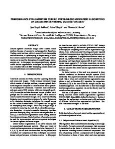
5.4.1 Production hardware A The production hardware A is a system with two CPUs, so a load-dependent center with m=2 was used to describe the CPU as in (4-12). CPU service time values were transformed to match the faster CPU using the transformation factor obtained from the transformation analysis as described earlier. The service time values for client and other resources were not touched. It was assumed that the CPU utilization of the system could reach 100% and that increasing load would not affect the CPU service time. The model was solved and the results from the model were compared with the measured performance are shown in Figure 5.4. The figure shows that the measured performance falls into the region predicted by the model. With high load the measured response time is quite close to the projected maximum response time and measured throughput is quite close to the projected minimum throughput.
56
R
Rmeas Rmin Ravg Rmax 1
2
3
4
5
6
7
8
9
10
11
12
X
n
Xmeas Xmin Xavg Xmax 1
2
3
4
5
6
7
8
9
10
11
12
n
Figure 5.4. Production hardware A model results compared with results from measurement. The figure shows response time (R) and system throughput (X) as a function of number of threads (n).
The comparison of CPU service time S in Figure 5.5 shows that the average value used in the model was very close to the actual, measured service time. The utilization comparison from the same figure shows that the CPU utilization U did not reach 100% as expected in the model, but did stop at 93%. This utilization limit is the reason why the model resulted in better performance measures than the actual system. There are two possible reasons this observed utilization limit. Firstly, processes that are note included in the model consume some CPU capacity. The second reason is that some limit prevents the software to fully utilize the CPU.
57
S
Smeas Smin Savg Smax 1
2
3
4
5
6
7
8
9
10
11
12
U
n
Umeas Umin Uavg Umax 1
2
3
4
5
6
7
8
9
10
11
12
n
Figure 5.5. Model CPU service time (S) and CPU utilization (U) plotted with different number of threads (n) compared with measured values on production platform A.
5.4.2 Production hardware B The production hardware B is a system with eight CPUs, so a load-dependent center with m=8 was used to describe the CPU as in (4-12). CPU service time values were transformed to match the faster CPU as described earlier. The service time values for client and other resources were not touched. It was assumed that the CPU utilization of the system could reach 100% and that increasing load would not affect the CPU service time. The model was solved using the MVA algorithm. The results from the model compared with the measured performance are shown in Figure 5.6. The figure shows that the measured performance remained within the limits predicted by the model when the load was low, but with high load the measured per-
58
formance dived below the model prediction. To study reason for this the CPU service time values used in the model and the CPU utilization obtained from the model are
R
compared with the measured values. This comparison is shown in Figure 5.7.
Rmeas Rmin Ravg Rmax 1
2
3
4
5
6
7
8
9
10
11
12
13
14
15
16
17
18
19
20
X
n
Xmeas Xmin Xavg Xmax 1
2
3
4
5
6
7
8
9
10
11
12
13
14
15
16
17
18
19
20
n
Figure 5.6. Production hardware B model results compared with results from measurement. Figure shows response time (R) and system throughput (X) as a function of number of threads (n).
The comparison shows that the measured CPU service time increased steadily with the load. This kind of behavior was unexpected and was not observed on other hardware used in the thesis. It is also shown that the CPU utilization of the real system did not reach the total capacity of 100% assumed by the model, but instead it stopped at 87%. The total CPU utilization of the system was measured to be at 90% with during the high load. This means that when 87% of the CPU capacity was used for the actual work, other processes consumed 3% and 10% of the capacity remained unused for unknown reason. It would mean an increase of 10% in system throughput if the unused capacity could have been utilized.
59
S
Smeas Smin Savg Smax 1
2
3
4
5
6
7
8
9
10
11
12
13
14
15
16
17
18
19
20
U
n
Umeas Umin Uavg Umax 1
2
3
4
5
6
7
8
9
10
11
12
13
14
15
16
17
18
19
20
n
Figure 5.7. Model CPU service time (S) and CPU utilization (U) plotted with different number of threads (n) compared with measured values on production platform B.
To study the service time more in detail measured average CPU service time was compared to the observed system throughput. The assumption in modeling was that the CPU service time would not be dependent on the amount of load to the system, that is (3-12) would hold. However the comparison shown in Figure 5.8 indicates that the CPU service time is linearly dependent on the system throughput. This means that the amount of work that a CPU has to process per request increases as the throughput increases. If the measured service time is checked on a process level, it shows that most of the service time increase was caused by the core process, which had an increase of 100% in service time. Service times for the front-end and database processes increase also, but not significantly. The core process is a java process so the reasons for this kind of behavior might be an increase in garbage collection or some other activity that is required when the load is high. Intuitively this seems odd, since one would assume that the work done per request would actually decrease with high throughput since the overhead cost of the
60
work is divided among many requests instead of one. The increase might also be due to some inefficient algorithm or even a bug in the software. Since this kind of behavior was not observed on the smaller platforms it might be that it is somehow related to the hardware configuration, but since the increase is mainly caused by one process this is
S
unlikely.
Smeas Smin Savg Smax X
Figure 5.8. Measured CPU service time (S) with system throughput (X) on production hardware B.
5.5 Summary of the results Overall the modeling can be considered a success. It did describe the behavior of the system correctly and with correct parameter values the results would have been very close to the measured performance. Without the model the performance anomalies would have not been detected. Although the model failed to predict the performance for one of the
61
platforms correctly, the results did however provide useful information for the workings of the system. The models used assumed that the CPU behavior could be described by a single constant, the CPU service time, which would be independent of the load to the system. Also it was assumed that a multi CPU machine would scale perfectly compared with a single CPU machine. The results indicate that in most cases the constant CPU service time assumption is adequate and that the multiple CPUs machines do indeed scale well. The MVA algorithm used requires that the system under study satisfies the product form assumptions explained in section 3.2.3. Although it is difficult to verify that the actual system satisfies these assumptions, the results obtained in the thesis suggest that it is appropriate to use the MVA algorithm. The time complexity of the algorithm did not prove to be a problem since the number of service centers and customers was small. The limit on the CPU utilization should be taken into account in the future models and its cause should be studied in detail. The used algorithm should be modified to accept the utilization limit as an input parameter. The service time increase anomaly on platform B clearly showed that performance anomalies are impossible to predict and why model results are verified with measurement. It also suggests that performance measurement results should be checked against a simple model to discover such anomalies. On the production platform A the model predicted the system throughput with ±7% and the response time with ±13% accuracy. On the production platform B the corresponding accuracies were ±16% and ±15%. This inaccuracy is mainly caused by the uncertainty in the service time values. The inaccuracy for the predicted throughput on platform B is too large. The most time consuming activity in the modeling was the service time estimation because it required a lot of measurement. In order to improve the accuracy of the service time estimates and reduce the time consumed in conducting the measurement a better way to determine them should be studied. In the thesis the service times were determined using the average values of separately measured CPU utilization and system throughput. A more accurate and efficient way would be to use a single tool that would measure both throughput and utilization and derive the service time values per each interval. From the
62
software development point of view performance tests could be utilized to obtain the service time values. This would also benefit the performance tests since their results could be verified against the service time estimates.
63
6 Conclusions
The results from the modeling suggest that software performance can be described with queuing network models. The used model was relatively simple, but it did describe the performance behavior of the software appropriately. The system model was simplified since it only included one of the services provided by the subscriber database. The workload was simplified because the requests and subscriber data were artificially generated. The resource model was simplified since CPU was the only hardware resource included. To make the model more realistic other services of the subscriber database should be included in the model as different customer classes. To solve such model requires an MVA algorithm for multiple customer classes [9] instead of the single class MVA used in the thesis. Also adding more classes to the model will increase the inaccuracy of the results [11]. The reason for why the system was studied with steady, artificial load is that it simplifies the analysis and that the performance requirements and tests assume such load. And since there was no information available about the traffic in real environment, a more complex workload representation would not be any better. The model could be extended to include other hardware resources. If the model is extended to include write services offered by the subscriber database the disk subsystem has to be included in the model. This would make the modeling more challenging since the performance behavior of the disk subsystem is more complex than the CPU performance behavior. The main challenge in the thesis was in the estimation of model service time values. Firstly, the values were too inaccurate for a system with high throughput. Secondly, there was no single tool available for obtaining the estimates, therefore several separate tools had to be used, which made the task more difficult, time consuming and the results even
64
more inaccurate. Finally, the service times were averages over long period. It might be useful if they could be measured per request. In software development performance testing would be a good way to obtain service time estimates. A similar model as the one used in this thesis could also be utilized in the development of future versions of the subscriber database. The difference is in the service time estimation. In the early phases of development service times are estimated using benchmarks, prototypes, expert's opinion and measurement data from earlier versions. Since the service time would be a combination of smaller pieces obtained by different methods, a more detailed model is required. The software execution model described in chapter 4.4.1 is one alternative for such a detailed description. During the development the service time values could be estimated more accurately as parts of the system would become complete and the performance could be measured. Transformation analysis might be required to transform the estimates to a different platform. The model could then be solved with the techniques described in this thesis. The basic performance modeling techniques utilized in the thesis can be applied for a wide variety of purposes like comparison of design alternatives, hardware capacity studies and validation of performance measurement data. Performance modeling is respectable performance evaluation technique, which can reduce the performance risks in software development. It does not exclude other techniques like measurement but is at best when it is used with them to explain the performance behavior of the system. Even if it does not provide accurate results, it helps in developing a deeper understanding on the performance of the system.
65
References: [1]
Cockcroft A., Richard P., "Sun Performance and Tuning : Java and Internet", 1998, Sun Microsystems Press, Palo Alto
[2]
Cooper, R. P., "Introduction to Queuing Theory", 1981, Elsevier, New York
[3]
Denning P. J., Buzen J. P., “The operation analysis of queuing network models”, Computing Surveys, vol. 10, September 1978, 225-261
[4]
Doebelin E. O., “Engineering experimentation: planning, execution, reporting”, 1995, McGraw-Hill, New York
[5]
Evans M., Hastings N., Peacock B., "Statistical Distributions", 2000, John Wiley & Sons, New York
[6]
Jacobson P. A., Lazowska E. D., “Analyzing queuing networks with simultaneous resource possession”, Communications of the ACM, vol. 25, February 1982, 142-151
[7]
Jain R., “The art of computer systems performance analysis: Techniques for experimental design, measurement, simulation and modelling”, 1991, John Wiley & Sons, New York
[8]
Java Programming Language, http://java.sun.com/, (checked 11.04.2003)
[9]
Kant, K, “Introduction to computer system performance evaluation”, 1992, McGraw-Hill, New York
[10]
Kreyzig E., “Advanced engineering mathematics”, 1988, John Wiley & Sons, New York
[11]
Lazowska E. D., Zahorjan J., Graham G. S. and Sevcik K. C., “Quantitative system performance: computer system analysis using queuing network models”, 1984, Prentice-Hall, New Jersey
[12]
Little, J. D. C., “The proof of relation N = λT”, Operations Research, vol. 9, May 1961, 383-387
66
[13]
Menascé D. A., "Software, performance, or Engineering?", Proceedings of the 3rd international workshop on software and performance in Rome 2002, 2002, 239-242
[14]
Nelson R., “Probability, stochastic processes, and queuing theory : the mathematics of computer performance modeling”, 2000, Springer-Verlag, New York
[15]
Pattipati K. R., Kostreva M. M., Teele J. L., ”Approximative mean value analysis algorithms for queuing networks: existence, uniqueness and convergence results”, Journal of the ACM, vol. 37, July 1990, 647-673
[16]
OMG Unified Modeling Language specification, http://www.uml.org, (checked 03.04.2003)
[17]
Oracle Corporation, http://www.oracle.com, (checked 03.04.2003)
[18]
Patterson D. A., Hennessy J. L., "Computer organization and design: the hardware/software interface", 1998, Morgan Kaufmann Publishers, San Francisco
[19]
Pooley, R., King, P., “The unified modeling language and performance engineering”, lEE Proceedings-Software, vol. 146, February 1999, 2-10
[20]
Sauer C. H., Chandy K. M., “Computer systems performance modelling”, 1981, Prentice-Hall, New Jersey
[21]
Schmietendorf A., Dimitrov E., Dumke R. R., “Process models for the software development and performance engineering tasks”, Proceedings of the 3rd international workshop on software and performance in Rome 2002, 2002, 211-218
[22]
Sensitivity analysis forum, http://sensitivity-analysis.jrc.cec.eu.int, (checked 03.05.2003)
[23]
Smith C. U., Williams L. G., "Software performance engineering: A case study including performance comparison with design alternatives", IEEE Transactions on software engineering, vol. 19, July 1993, 720-741
[24]
Smith C. U., Williams L. G., “Performance solutions: a practical guide to creating responsive, scalable software”, 2002, Addison-Wesley, Boston
[25]
Solaris developer connection, http://sundc.sun.com, (checked 22.04.2003)
67
[26]
Stallings W., “Operating systems: internals and design principles”, 1998, Prentice-Hall, New Jersey
[27]
Zahorjan J., Sevcik K. C., Eager D. L., Galler B., "Balanced Job Bound Analysis of Queuing Networks", Communications of the ACM, vol. 25, February 1982, 134-141
68