Magnetic Resonance in Medicine 53:1393–1401 (2005)
Partial Fourier Partially Parallel Imaging Mark Bydder* and Matthew D. Robson The techniques of partial Fourier (PF) and partially parallel imaging have been combined using a constrained reconstruction technique. The benefits compared with the individual techniques are reduced imaging time and/or an increase in signalto-noise ratio. Low-resolution phase maps and coil sensitivities may be obtained using autocalibration or from a prescan followed by additional processing. Minor phase artifacts that are introduced by relying on conjugate symmetry can be reduced using a novel regularization scheme to vary the degree to which PF is used in the reconstruction. A nonrectilinear reconstruction algorithm is presented and the potential for motion artifact reduction is investigated using robust reconstruction. Magn Reson Med 53:1393–1401, 2005. © 2005 Wiley-Liss, Inc. Key words: partial Fourier; partially parallel imaging; conjugate symmetry; constrained least squares; regularization
The magnetic resonance (MR) techniques of partial Fourier (PF) and partially parallel imaging (PPI) permit decreased acquisition times by reducing the amount of phase encoding needed to image an object (1– 4). Speed-up factors of around 2 and 4, respectively, have been widely attained and even higher values for PPI are becoming commonplace. In principle, PPI can provide an almost unlimited reduction in acquisition time although in practice it suffers from decreasing signal-to-noise-ratio (SNR) at higher speed-up factors, largely as a result of noise amplification, which becomes prohibitive above a critical value (5). In contrast to PPI, which samples k-space more sparsely to gain higher speed-up factors, the strategy with PF is to sample at full density but over a reduced area of k-space. This leads to only a moderate increase in noise although the asymmetrical sampling of k-space can introduce artifacts where there are fast phase variations in the image. Nevertheless, both techniques are commonly used when the need for short acquisition times outweighs the SNR and artifact penalties. A number of studies have proposed the idea of applying both speed-up methods simultaneously, using a variety of k-space sampling patterns and reconstruction algorithms to recover the image (3,6 –14). The basic idea is to acquire just over half of k-space but at less than the Nyquist criterion so there are elements of both PF and PPI in the acquisition, as illustrated in Fig. 1a– c. The phase maps and coil sensitivities required by the reconstructions may be acquired as part of the measurement scan using autocalibration, i.e., fully sampling the low frequencies of k-
1 Department of Radiology, Magnetic Resonance Institute, UCSD Medical Center, San Diego, California, USA. 2 Centre for Clinical Medical Resonance Research, John Radcliffe Hospital, University of Oxford, Oxford, United Kingdom. *Correspondence to: Mark Bydder, Magnetic Resonance Institute, Department Radiology, UCSD Medical Center, 200 West Arbor Drive, San Diego CA 92103-8756, USA. E-mail:
[email protected] Received 23 March 2004; revised 5 January 2005; accepted 10 January 2005. DOI 10.1002/mrm.20492 Published online in Wiley InterScience (www.interscience.wiley.com).
© 2005 Wiley-Liss, Inc.
space (Fig. 1d), or from a separate prescan (described below). A variant is to acquire data over the whole of k-space but with the high frequencies arranged so they are not in conjugate symmetric pairs, for example, the odd lines on one side of k-space and the even lines on the other (Fig. 1e). It is often preferable to measure coil sensitivities using a prescan since this can be performed using a fast or inherently high SNR sequence. Prescans are adequate for the PPI reconstruction since only the relative coil sensitivities are required; however, the PF reconstruction requires an absolute measure of the phase and this must be obtained by additional processing. A detailed procedure in (9) describes a way of doing this when combined with PF and PPI sampling strategies—there are in fact two stages involved: obtaining coil sensitivities with suitable phase and obtaining the final image, although the processes overlap somewhat. A variant of the method in Ref. (9) is outlined below. Obtaining Coil Sensitivities/Phase Maps A fully sampled 64 ⫻ 64 prescan is made. The images are low-pass filtered and normalized with a square root sum-of-squares (SOS) divisor to provide coil sensitivities. ii. An undersampled measurement scan is made at 256 ⫻ 256 resolution using sampling pattern 1c with line spacing of 2 and 9/16 coverage of k-space. iii. The central 1/8 portion of (ii) is extracted and Fourier transformed to the image domain. A sensitivity encoding (SENSE) (3) reconstruction is performed on this data using the coil sensitivities from (i). iv. Each of the coil sensitivities from (i) is multiplied by the image produced in (iii). These are low-pass filtered and normalized with a SOS divisor to provide new coil sensitivities. i.
Reconstructing the Undersampled Data v. A PF correction is performed on the k-space data in (ii) by doubling the amplitude of any data point that has no conjugate symmetric counterpart, i.e., the outer lines. vi. The data in (v) are Fourier transformed to the image domain. vii. A SENSE reconstruction is performed on the data in (vi) using coil sensitivities from (iv). viii. The real part of the image is taken. These steps produce an image that has some Gibbs ringing artifact, which arises from using a step filter to weight the k-space data rather than a smoothly varying function (Fig. 2a). As discussed in Ref. (1), filtering with a linear ramp removes this artifact (Fig. 2b) but may also increase the noise since the step function is optimal for SNR. In Ref.
1393
1394
Bydder et al.
FIG. 1. Schematic diagrams of rectilinear k-space. (a) PF sampling. (b) PPI sampling. (c) PFPP. (d) Autocalibrating PFPP. (e) Autocalibrating, sampling both sides of k-space.
(9) and the other articles referred to above, the images presented were free of Gibbs artifact; however, the specific implementation details were not always given so it is difficult to know what processing was applied. In any case, it is unclear whether any filter could be considered “optimal” since the theoretically optimal choice results in artifacts. Two recent studies have taken a different approach to combining PF and PPI by posing the reconstruction as an inverse problem and using constraints to impose the desired properties on the solution (15,16). The resulting image must satisfy both the phase requirements of PF and the coil sensitivity requirements of PPI. The formalism provides a clear idea of what the reconstruction is trying to achieve—namely minimize a specific measure of the error, or objective function. The inverse problem approach to combining PF and PPI is referred to here as partial Fourier partially parallel (PFPP) imaging. In this study, methods are presented based on general formulations of PPI, such as SENSE and sensitivity profiles from an array of coils for encoding and reconstruction in parallel (SPACE RIP) (4). A novel approach for combining PF as a regularization parameter in the PPI reconstruction is described, permitting a trade-off between the artifacts associated with PF and the noise amplification associated with PPI. The scope for artifact reduction is investigated by suppressing corrupt data points and relying on conju-
gate symmetry (PF) and/or neighboring data points from different coils (PPI) to generate replacement data. Phantom and in vivo results are presented. THEORY Conjugate symmetry, also known as Hermitian symmetry, is the property that s共k) ⫺ s共 ⫺ k)*⫽0,
[1]
where s(k) is a k-space data point at position k and * denotes complex conjugation. To incorporate this property into PPI, the SENSE equation is initially written as s ⫽ B,
[2]
where B is a sensitivity matrix, is a vector of image pixels to be reconstructed, and s is a vector of acquired k-space samples from n ⱖ 1 coils. In the image domain, conjugate symmetry implies that the object is pure real, i.e., Im{}⫽0. This property can be incorporated into Eq. [2] by separating into real and imaginary parts (17a) and forming a constrained least squares equation [18],
FIG. 2. Phantom data set (phaseencode direction left–right) with separate coil sensitivities using kspace sampling 1c with line spacing of 2 and 80 lines in total. (a) King’s method with a step filter in k-space. (b) King’s method with a linear ramp filter. (c) PFPP method with ⫽ 0.8. (d) Amplitude of the difference between (a) and the “gold standard” image. (e) Difference between (b) and the gold standard image. (f) Difference between (c) and the gold standard image. Images (a– c) and (d–f) are windowed identically.
PFPP Imaging
1395
冋 册 冋 Re{s} Im{s} 0
⫽
Re{B} Im{B} 0
Im{⫺B} Re{B} I
册冋
Re{} Im{}
册
[3]
algorithm in Ref. (21) for solving Eq. [3] is described in the Appendix. Robust PFPP
where I is the identity matrix and is a scalar used to strengthen/weaken the constraint. For the constraint to be meaningful there must be some reason to expect the object to be real since in MR imaging it is not usually the case. Hence, a phase correction is applied to during the reconstruction using phase maps acquired separately or by autocalibration, as described in Ref. (16). With specific coil sensitivities and processing, the phase correction is implicit in B; for example, when the coil sensitivities are obtained from the method described in the introduction or autocalibration and a SOS coil modulation is used. These phase maps will generally be of low spatial resolution. Examining the limiting cases of Eq. [3], when is zero, Eq. [3] is equivalent to PPI (Eq. [2]), which is prone to excessive noise at high speed-up factors. When is large the reconstruction relies on conjugate symmetry as well as the coil sensitivities, which gives a result more or less identical to that of Ref. (16), since Im{} becomes negligible and may be excluded from the equation. The benefits of this approach demonstrated in Ref. (16) are reduced noise and higher potential speed-up factors. However, there is a price to pay for this gain and that is that the low-resolution phase maps are unlikely to correct the full resolution images perfectly. Therefore, conjugate symmetry will not hold exactly and artifacts will be introduced where there are fast phase variations in the image. Intermediate values of allow a trade-off between the noise of PPI and the artifacts of PF so that at least some noise can be reduced for a negligible increase in artifact. Nonrectilinear PF and PPI To date the PFPP techniques have been implemented for rectilinear k-space sampling only, although PF and PPI have been used separately with arbitrary sampling strategies (e.g., 19 –21). Nonrectilinear sampling is important for obtaining particular image contrasts (22) and can be resistant to motion artifacts when there is a high degree of oversampling at the center of k-space. The down side is that the edges of k-space often remain undersampled, which gives rise to characteristic aliasing artifacts. The advantages and disadvantages of nonrectilinear acquisitions appear to be well matched for their use with PFPP reconstruction, since the densely sampled center of kspace provides calibration data while the sparsely sampled edges may benefit from the combined ability of PF and PPI to interpolate into gaps in k-space. The matrix approach of Eq. [3] is general to any k-space trajectory, although the large amount of computer processing required means it is practical only for rectilinear data sets where the reconstruction can be split along the frequency-encode direction into multiple smaller reconstructions (4). An alternate approach that does not involve large matrices is to effect the operation of B on a vector using gridding and Fourier transforms, combined with an iterative conjugate gradient solver (21). A generalization of the
The least squares solution of Eq. [3] minimizes the objective function 储s ⫺ B储 22 ⫹ 2储Im{}储 22
[4]
where 储 䡠 储2 is the 2-norm. This has some similarity with zeroth-order regularization (17b), which can also be included by minimizing the objective function 储s ⫺ B储 22 ⫹ 2储Im{}储 22 ⫹ ␦ 2储储 22
[5]
for some scalar ␦. Another way to solve these equations is to minimize an objective function other than the 2-norm— typically minimizing the p-norm with 1 ⱕ p ⬍ 2 may be used as a way to suppress outliers in s (17c). Since the variance is minimized when p ⫽ 2, any other objective function will decrease the SNR, although this is offset against the potential decrease in artifacts. Iteratively reweighted least squares is a method for minimizing arbitrary objective functions and has been implemented here using the Huber estimator, in the same way as described in Ref. (23). In previous artifact reduction work, PF and PPI have been used separately to replace corrupt k-space data points by using conjugate symmetry (19) or making linear combinations of the data from different coils (24). The two sources of redundancy are complementary insofar as PF is nonlocal (opposite side of k-space) while PPI is local (nearby points in k-space). This has significance for artifact reduction since the consistency of each data point will be determined from two different sources, although near the center of k-space the data points used by PF and PPI coincide so they are not complementary in this region. METHODS Data were acquired on a Sonata 1.5-T scanner (Siemens, Erlangen, Germany) using three elements of a spine array or a four- or eight-element head array (MRI Devices, Gainesville, FL, USA). Rectilinear-sampled spin echo sequences (TR 500 ms, TE 16 ms) were used for the measurement scans and a fast imaging with steady state precession (TrueFISP) sequence (TR 3.6 ms, TE 1.8 ms) for the prescan. Radial sampling was performed using a centerout ultrashort TE sequence (TR 1000 ms, TE 0.1 ms) as described in Ref. (22). All images were 256 ⫻ 256 resolution and decimated postacquisition to provide undersampled data sets. Coil sensitivities were either obtained from the prescan or derived from the measurement data using autocalibration. In the latter case the autocalibration data were included in the reconstruction. Coil sensitivity images were low-pass filtered using a Kaiser window and normalized by dividing by the SOS of all the coil sensitivity images. Therefore, the largest amplitude elements of 〉 were of the order 1. This provides a reference scale for choosing , since is now expressed as
1396
Bydder et al.
Table 1 The Error (Eq. [6]) versus Regularization Parameter for the Data Sets of Figs. 2, 3, and 4 0.0 0.4 0.8 1.6 109
Error Fig. 2c
Fig. 3a
Fig. 3c
Fig. 4b
Fig. 4e
0.183 0.026 0.025 0.025 0.026
0.189 0.060 0.043 0.039 0.038
0.106 0.039 0.038 0.038 0.038
0.094 0.073 0.068 0.076 0.109
0.258 0.103 0.103 0.104 0.119
a fraction of the root-mean-square (RMS) of the coil sensitivities. If a different divisor than the SOS is used (or no divisor), must be scaled by the RMS of those coil sensitivities to remain consistent (note: the RMS of the coil sensitivities using a SOS divisor is 1). An alternative scaling might be to use the maximum amplitude or the mean amplitude, but none has any particular significance. The SPACE-RIP (4) algorithm was modified as indicated by Eq. [3[rsqab] and the iterative SENSE (21) algorithm modified as described in the Appendix. Apart from the images in Fig. 2 all results were obtained from the latter method. Regridding of the nonrectilinear k-space samples was performed by convolution with a Kaiser–Bessel kernel of width 4, oversampling factor 1.5, and shape parameter ␣ ⫽ 2.05 ⫻ width (25). A bilinear kernel was used for the rectilinear data sets. Density and intensity corrections were not performed. A fixed number of 100 conjugate gradient iterations was used giving tolerances ⬍10⫺4 (see
Appendix). Reconstruction times were approximately 1 min per image on a 3-GHz P4 processor running MATLAB (The Mathworks, Natick, MA, USA). To quantify the accuracy of the reconstructed images, comparisons were made to a “gold standard” image, which was taken to be the SOS of the fully sampled data set. The fractional RMS of the difference was calculated using Eq. [6], excluding regions containing background noise.
Error ⫽
冑
⌺(兩Image兩 ⫺ 兩Gold兩) 2 ⌺兩Gold兩 2
[6]
RESULTS Figure 2 shows phantom images from the spine coil reconstructed using the method described in the introduction, based on Ref. (9). Separate coil sensitivities with resolution 64 ⫻ 64 were used. For the measurement data, k-space sampling 1c was used with line spacing of 2 and a total of 80 lines: (Fig. 2a) using a step filter in k-space; (Fig. 2b) using a linear ramp filter to remove Gibb’s artifact; (Fig. 2c) reconstructed from the same data using PFPP with ⫽ 0.8. Clearly the image produced by this method will depend on the value chosen for . The error determined by Eq. [6] for several values of is given in Table 1, revealing a broad minimum of 0.025 around ⫽ 0.8. For comparison the errors for the images in Fig. 2a and b are 0.028 and 0.043, respectively. Difference images (using the SOS of the fully sampled data as the gold standard image) are shown in Fig. 2d–f.
FIG. 3. Phantom data set (phase-encode direction up– down). (a) and (b) show images from autocalibrating k-space sampling 1e using outer line spacing of 4, 48 center lines, and 100 lines total with ⫽ 0 and 109, respectively. (c) shows the image using same number of k-space lines but with sampling pattern 1d (outer line spacing of 2, 48 center lines, and 100 lines total with ⫽ 109). (d) shows the effect of using fewer central lines (outer line spacing of 4, 16 center lines, and 76 lines total).
PFPP Imaging
1397
FIG. 4. In vivo data set (phase-encode direction left–right) with autocalibrating k-space sampling pattern 1e using outer line spacing of 4 and 32 center lines (88 lines in total). For comparison, (a) is the fully sampled “gold standard” image for this data set. (b) shows the undersampled data set reconstructed with ⫽ 0, (c) ⫽ 0.8, and (d) ⫽ 109. The arrows show an instance of how phase artifacts are aliased into the image from distant vessels. (e) Surface plot of RMS error versus (range 0 to 1.6) and ␦ (range 0 to 0.5), see Eq. [5]. (f) The image at the minimum error ( ⫽ 0.72, ␦ ⫽ 0.24). (g) The image at ⫽ 0.3, ␦ ⫽ 0.2, which may be preferable to the one at minimum error. (h) shows the image using same number of k-space lines but with sampling pattern 1d (outer line spacing of 2, 32 center lines, and 88 lines total with ⫽ 0.8).
Figure 3 shows phantom images from the eight-element head coil reconstructed using autocalibrating sampling pattern 1e: (Fig. 3a) ⫽ 0 and (Fig. 3b) ⫽ 109 with 48 central lines, outer line spacing of 4, and 100 lines in total. Note the considerable reduction in noise in Fig. 3b, which translates into reduced error (Table 1). For this data set, the error is a monotonically decreasing function of . In Fig. 3c the same number of k-space lines was used but with sampling pattern 1d ( ⫽ 109, outer line spacing of 2, 48 center lines, 100 lines in total). The error also decreases with (Table 1) and is marginally lower than when using sampling pattern 1e. Figure 3d shows an example of the residual aliasing that can occur if the calibration data have insufficient resolution to adequately describe the coil sensitivities and phase ( ⫽ 109, outer line spacing of 4, 16 central lines, 76 lines in total). Figure 4 shows in vivo data from the eight-element head coil. Figure 4a shows the fully sampled image reconstructed using the SOS. Figure 4b– d shows images reconstructed by PFPP for ⫽ 0, ⫽ 0.8, and ⫽ 109 using an autocalibrating sequence (sampling pattern 1e) with 32 central lines and an outer line spacing of 4 (88 lines in total). Although the noise is reduced most in Fig. 4d, artifacts are introduced in areas that have fast phase variations, e.g., due to blood flow, and these artifacts are aliased onto other parts of the image (see arrows). Table 1 lists the error for different values of , revealing a minimum ⫽ 0.8. A search was also performed over and ␦. The global minimum of 0.064 was found at ⫽ 0.72 and ␦ ⫽ 0.24 (see Fig. 4e), which is lower than that found by varying alone (minimum 0.068 at ⫽ 0.80) and ␦ alone (minimum 0.069
at ␦ ⫽ 0.34). The image at the global minimum is shown in Fig. 4f. Arguably, the image contains a higher level of artifact than might be preferred by visual inspection; for example, the image at ⫽ 0.3 and ␦ ⫽ 0.2 shown in Fig. 4g contains almost no visible artifact at a cost of only slightly greater noise. Using the same amount of data but a different sampling pattern, Fig. 4h shows an image reconstructed by PFPP with ⫽ 0.8 using k-space sampling pattern 1d (32 central lines, outer line spacing of 2, and 88 lines in total). The error has broad minimum from ⫽ 0.30 to 2.0 which increases slowly as 3 ⬁. Despite the higher overall error, the image using this sampling pattern is arguably preferable to the ones shown in Fig. 4b– d. However, it must rely wholly on PF to fill one side of k-space, which makes it vulnerable to phase artifacts, whereas sampling pattern 1e can rely on PF and/or PPI across the whole of k-space and hence it enables the trade-off between phase artifacts and noise. Figure 5 shows images reconstructed from nonrectilinear center-out radial k-space sampling. Coil sensitivities were regridded from the central 48 ⫻ 48 region of k-space. Figure 5a– c shows simulation results from a numerical Shepp–Logan phantom using a single coil data set: (Fig. 5a) 86 spokes with ⫽ 0; (Fig. 5b) 85 spokes with ⫽ 0; (Fig. 5c) 85 spokes with ⫽ 109. There are two effects that are illustrated in these images—the first is a reduction in aliasing that comes from using an odd number of equally spaced radial spokes and the second is an increase in resolution that comes from invoking conjugate symmetry. As described in Ref. (20), the first effect is due to the fact that an odd number of
1398
Bydder et al.
FIG. 5. Results using a nonrectilinear radial k-space trajectory. (a) Shepp–Logan numerical phantom using 86 spokes with ⫽ 0. (b) 85 spokes with ⫽ 0. (c) 85 spokes with ⫽ 109. (d) Phantom data set using 4 coils and 127 radial spokes with ⫽ 0. (e) The same data with ⫽ 109. (f) Fourier transform of (d). (g) Fourier transform of (e).
spokes produces a complex point-spread function, which has much less coherent aliasing than the real point-spread function produced by an even number of spokes. The second effect is due to the k-space data being essentially reflected across the origin, so when the spokes are positioned asymmetrically (e.g., by using an odd number of spokes) the reflected spokes align with gaps on the other side of k-space and the final image is comparable with an image obtained from a greater number of spokes. Reconstructions were performed using actual MR data from a four-element head coil composed of 127 radial spokes. Figure 5d shows the image reconstructed with ⫽ 0. Figure 5e is the same data set but with ⫽ 109. Figure 5f shows the Fourier transform of Fig. 5d. Figure 5g shows the Fourier transform of Fig. 5e. The Fourier transforms show how data are reconstructed only near to a radial spoke and that invoking conjugate symmetry effectively doubles the number of spokes. As in the simulation images, the effect of using a nonzero is increased resolution, although high-frequency aliasing artifacts are introduced. These artifacts are caused by certain areas of the image violating the smooth phase assumption and compounded by being aliased to other parts of the image, as seen in the rectilinear case (Fig. 4d). Decreasing the value of provides a trade-off between the increase in resolution and the phase artifacts. Figure 6 shows phantom data from the eight-element head coil using autocalibration (32 lines) and full k-space sampling, in which simulated motion artifacts have been introduced into the data (see below). Figure 6a shows the image reconstructed with ⫽ 0. Figure 6b shows the
Huber estimator and ⫽ 0. Figure 6c was reconstructed with the Huber estimator and ⫽ 109. The motion artifacts are reduced in Fig. 6b and further reduced in Fig. 6c due to the increased redundancy in the data set. This verifies that PF and PPI together can enhance the outlier suppression ability of robust reconstruction. The motion artifacts were introduced by applying phase offsets randomly to 37 lines excluding the autocalibration lines, which corresponds to translations in the phase encode direction. As noted in Ref. (23), robust methods are only suited to removing localized errors in k-space (e.g., 1 or 2 consecutive lines) that comprise a modest fraction of the data set and it is important that the calibration data be free of motion artifact. These properties correspond to the concepts of “breakdown point” and “errors in variables” in robust statistics, although a detailed study of these methods is beyond the scope of the present work. Figure 7 demonstrates the case of undersampling in two directions, as in 3D or spectroscopic imaging (26), using data from the eight-element head coil. Figure 7a shows an image reconstructed from a 2 ⫻ 2-fold undersampled data set (i.e., 128 ⫻ 128 acquired points) using ⫽ 0. Figure 7b shows the same data set reconstructed with ⫽ 109, exhibiting reduced noise. It is also possible to acquire only 9/16 k-space in one direction to reduce the acquisition time at the cost of reduced SNR. DISCUSSION There is generally a trade-off between scan time and image quality. In the present method the maximum speed-ups
PFPP Imaging
1399
come from sampling one side of k-space with a large line spacing, which suffers from both PF phase artifacts and high PPI noise amplification. By sampling more densely, using more coils and/or sampling both sides of k-space, redundancy is built into the acquisition, which increases the SNR and allows a trade-off with phase artifacts using a free parameter (). The reconstruction procedure has sim-
FIG. 7. Undersampled in two directions with speed-up factor of 2 in both directions. (a) shows the image reconstructed using ⫽ 0 and (b) shows the same data reconstructed using ⫽ 109.
FIG. 6. Phantom data set with full k-space sampling (autocalibrating using 32 center lines and 256 lines in total) containing 37 corrupt outer lines. (a) Least squares PPI reconstruction ( ⫽ 0). (b) Robust PPI reconstruction ( ⫽ 0). (c) Robust PFPP reconstruction ( ⫽ 109).
ilarities with zeroth-order regularization of a linear system, which balances the accuracy of a solution with a priori knowledge/assumptions about the solution, e.g., that it be finite in magnitude (17b,27). In the present case the assumption is that the reconstructed (phase-corrected) image is pure real, which is plausible based on the successful adoption of PF techniques that make use of this assumption in clinical imaging. Several previous studies have proposed the idea of incorporating PF into PPI to increase imaging speed and/or improve SNR. In particular, King and Angelos (9) presented a method based on sequential application of PF and PPI and Willig-Onwuachi et al. (16) presented a phaseconstrained method that corresponds with the present technique for the case 3 ⬁. Samsonov and Kholmovski (15) earlier described a general technique that imposes a smooth phase constraint on the image rather than the zero phase constraint used here and in Ref. (16). The present technique (and that of Willig-Onwuachi et al.) must perform a phase correction during the reconstruction whereas the method of Samsonov and Kholmovski simply constrains the phase to be smooth, which may be a more direct way of obtaining the same result. Nonrectilinear trajectories are compatible with PFPP using a method based on an algorithm previously developed
1400
for PPI (21). Despite the increased effective sampling density from invoking conjugate symmetry (Fig. 5f and g) the difference in image quality between PPI and PFPP appears to be relatively small, amounting to a slight increase in resolution which is offset against an increase aliasing due to phase artifacts. The nonrectilinear PFPP algorithm can be used to reconstruct rectilinear data sets that are undersampled in two directions and in this case it provides a marked improvement over PPI alone (Fig. 7). Another potential use of PFPP imaging is in robust reconstruction, which identifies inconsistencies between data points in order to reduce motion artifacts (23). The technique essentially finds a consistent subset in the available data and uses only those data points to reconstruct the image. It is restricted by the need to obtain accurate calibration data and for a majority of the data to be consistent, which may be troublesome unless the patient is mostly stationary during the acquisition. However, when the conditions are met, the motion artifact reduction from PF and PPI combined is greater than with PPI alone (Fig. 6). Practical methods for choosing the regularization parameters have not been addressed in the present study, although clearly there is some noise reduction from using nonzero values for and ␦. Experiments with different coil arrays indicate that a value of around ⫽ 0.8 gives the minimum RMS error compared to the fully sampled image. Arguably, a lower value of produces more visually acceptable images since additional noise may be preferable to unusual artifacts. A practical approach for choosing the regularization parameters might be to use fixed “small” values (e.g., ⫽ 0.3 and ␦ ⫽ 0.2) that are unlikely to introduce artifacts in the image yet provide some of the benefit of reduced noise.
CONCLUSION A technique has been developed that combines PF with PPI by constraining PPI to produce a pure real image. A novel regularization scheme is used that allows a trade-off between noise amplification from PPI with phase artifacts from PF, which occur where there are fast phase variations in the image.
APPENDIX A conjugate gradient algorithm based on Ref. (21) is described. Forming the normal equations of Eq. [3] and expanding the RHS gives (after a little algebra) BHB ⫹ i2 Im{}. Hence the ⌱ term in Eq. [3] acts so as to add the quantity i2 Im{} to the vector BHB. Due to the decoupling of real and imaginary parts, this should not strictly be considered a complex vector but rather a real vector of twice the length that contains real and imaginary parts separately. The only outcome of this is that the imaginary part of the dot product must be discarded. For generality the algorithm presented below allows an initial estimate initial(e.g., from the calibration data) and a zeroth-order regularization parameter ␦ (cf. Eq. [5]). Stopping criteria may be used to terminate the iterations, for example, when rj Hrj /r0Hr0 reaches a certain tolerance.
Bydder et al.
⫽ initial d ⫽ initial r 0 ⫽ B Hs for j ⫽ 1,2. . . q ⫽ B HBd ⫹ i2 Im{d} ⫹ ␦2d if j ⫽⫽ 1 r1 ⫽ r0 ⫺ q d ⫽ r1 else ⫽⫹
r j Hrj d Re{dHq}
r j ⫹ 1 ⫽ rj ⫺
rj Hrj q Re{dHq}
d ⫽ rj ⫹ 1 ⫹
rj ⫹ 1Hrj ⫹ 1 d rj Hrj
end end
ACKNOWLEDGMENTS The authors thank Alexei Samsonov of the Departments of Radiology and Medical Physics, University of Wisconsin, for many helpful discussions. We also thank Ronald Ouwekerk of the Department of Radiology, Johns Hopkins University, for providing the numerical Shepp-Logan phantom (mriphantom.m).
REFERENCES 1. Noll DC, Nishimura DG, Macovski A. Homodyne detection in magnetic resonance imaging. IEEE Trans Med Imaging 1991;10:154 –163. 2. McGibney G, Smith MR, Nichols ST, Crawley A. Quantitative evaluation of several partial Fourier reconstruction algorithms used in MRI. Magn Reson Med 1993;30:51–59. 3. Pruessmann KP, Weiger M, Scheidegger MB, Boesiger P. SENSE: sensitivity encoding for fast MRI. Magn Reson Med 1999;42:952–962. 4. Kyriakos WE, Panych LP, Kacher DF, Westin CF, Bao SM, Mulkern RV, Jolesz FA. Sensitivity profiles from an array of coils for encoding and reconstruction in parallel (SPACE RIP). Magn Reson Med 2000;44:301– 308. 5. Wiesinger F, Pruessmann KP, Boesiger P. Inherent limitation of the reduction factor in parallel imaging as a function of field strength. IN: Proceedings of the 10th Annual Meeting of ISMRM, Honolulu, 2002. p 191. 6. Glover PM, Tokarczuk PF, Bowtell RW. A robust single-shot partial sampling scheme. Magn Reson Med 1995;32:74 –79. 7. Griswold MA, Jakob PM, Chen Q, Goldfarb JW, Manning WJ, Edelman RR, Sodickson DK. Resolution enhancement in single-shot imaging using SMASH. Magn Reson Med 1999;41:1236 –1245.
PFPP Imaging 8. Sodickson DK, Stuber M, Botnar RM, Kissinger KV, Manning WJ. SMASH real-time cardiac MR imaging at echocardiographic frame rates. In: Proceedings of the 9th Annual Meeting of ISMRM, Glasgow, Scotland, 1999. p 387. 9. King KF, Angelos L. SENSE with partial Fourier homodyne reconstruction. In: Proceedings of the 8th Annual Meeting of ISMRM, Denver, 2000. p 153. 10. Kellman P, Epstein FH, McVeigh ER. Adaptive sensitivity encoding incorporating temporal filtering (TSENSE). Magn Reson Med 2001;45: 846 – 852. 11. Griswold MA, Jakob PM, Heidemann RM, Nittka M, Jellus V, Wang J, Kiefer B, Haase A. Generalised autocalibrating partially parallel acquisitions. Magn Reson Med 2002;47:1202–1210. 12. Heidemann MR, Griswold MA, Kiefer B, Nittka M, Wang J, Jellus V, Jakob PM. Resolution enhancement in lung 1H imaging using parallel imaging methods. Magn Reson Med 2003;49:391–394. 13. Li BS, Chen Q, Li W, Lingamneni A, Angelos L, Polzin JA, Edelman RR. Single-shot FIESTA single-breath-hold whole-heart MRI with 4X parallel imaging. In: Proceedings of the 11th Annual Meeting of ISMRM, Toronto, Canada, 2003. p 380. 14. Klarhofer M, Dilharreguy B, van Gelderen P, Moonen C. A PRESTO SENSE sequence with alternating partial Fourier encoding for rapid 3D MRI time series. In: Proceedings of the 11th Annual Meeting of ISMRM, Toronto, Canada, 2003. p 740. 15. Samsonov AA, Kholmovski EG. Method for quality improvement of images reconstructed from sensitivity encoded data. In: Proceedings of the 10th Annual Meeting of ISMRM, Honolulu, 2002. p 2408. 16. Willig-Onwuachi JD, Yeh EN, Grant AK, Ohliger MA, McKenzie CA, Sodickson DK. Phase-constrained parallel MR image reconstruction using symmetry to increase acceleration and improve image quality. In: Proceedings of the 11th Annual Meeting of ISMRM, Toronto, Canada, 2003. p 19.
1401 17. Press WH, Teukolsky SA, Vetterling WT, Flannery BP. In: Numerical recipes in C, 2nd ed. Cambridge: Cambridge University Press; 1992; (a) p 50, (b) p 808, (c) p 699. 18. Golub GH, van Loan CF. In: Matrix computations. Baltimore, MD: Johns Hopkins University Press; 1983. p 410. 19. Takahashi A, Glover GH. Half Fourier spiral image reconstruction. In: Proceedings of the 5th Annual Meeting of ISMRM, Vancouver, Canada, 1997. p 135. 20. Hargreaves BA, Pauly JM, Nishimura DG. Comparison of even and odd projection-reconstruction sampling strategies. In: Proceedings of the 7th Annual Meeting of ISMRM, Philadelphia, 1999. p 658. 21. Pruessmann KP, Weiger M, Bornert P, Boesiger P. Advances in sensitivity encoding with arbitrary k-space trajectories. Magn Reson Med 2001;46:638 – 651. 22. Robson MD, Gatehouse PD, Bydder M, Bydder GM. Magnetic resonance: an introduction to ultrashort echo-time imaging. J Comput Assist Tomogr 2003;27:825– 846. 23. Bydder M. The use of robust methods to reduce image artefacts. In: Proceedings of the 11th Annual Meeting of ISMRM, Toronto, Canada, 2003. p 482. 24. Bydder M, Larkman DJ, Hajnal JV. Detection and elimination of motion artefacts by regeneration of k-space. Magn Reson Med 2002;47:677– 686. 25. Matej S, Fessler JA, Kazantsev IG. Iterative tomographic image reconstruction using Fourier-based forward and back-projectors. IEEE Trans Med Imaging 2004;23:401– 412. 26. Dydak U, Weiger M, Pruessmann KP, Meier D, Boesiger P. Sensitivityencoded spectroscopic imaging. Magn Reson Med 2001;46:713–722. 27. King KF, Angelos L. SENSE image quality improvement using matrix regularization. In: Proceedings of the 9th Annual Meeting of ISMRM, Glasgow, Scotland, 2001. p 1771.