Systems Engineering Group Department of Mechanical Engineering Eindhoven University of Technology PO Box 513 5600 MB Eindhoven The Netherlands http://se.wtb.tue.nl/
SE Report: Nr. 2010-04
Partial Bisimulation J.C.M. Baeten D.A. van Beek B. Luttik J. Markovski J.E. Rooda 1
ISSN: 1872-1567
SE Report: Nr. 2010-04 Eindhoven, April 2010 SE Reports are available via http://se.wtb.tue.nl/sereports
Abstract We investigate partial bisimulation preorder, a behavioral preorder that is coarser than bisimulation equivalence and finer than simulation preorder. Partial bisimulation preorder is parameterized with a subset of actions; if two processes are related, then transitions labeled with an action in this subset need to be simulated in both directions, whereas transitions labeled with an action outside the subset need to be simulated in one direction only. The parameter is employed to define a notion of controllability, and discuss the supervisory control synthesis problem in a process-theoretic setting. Our notion of controllability improves on the current definition of controllability of nondeterministic discrete-event systems, which is given in terms of traces and/or refusal sets. We present a sound and ground-complete axiomatization of the partial bisimulation preorder and a modal characterization. We also provide for a partitioning algorithm that computes the partial bisimulation equivalence, and can serve as a minimization procedure in a supervisory control setting. The algorithm is based on partition pairs and it employs Paige-Tarjan optimization, which makes it suitable as a basis for an efficient algorithm for simulation minimization as well.
1 Introduction To keep products competitive, producers need to optimize development costs and minimize time-to-market, while satisfying the ever-changing market demands for higher quality, better performance, new functionalities, improved safety, and ease of use. This puts high demands on the development of control software. Traditionally, software engineers write control software based on specification documents that contain informal requirements. This is a timeconsuming error-prone process, since the requirements are often ambiguous and, moreover, they constantly change during the product development. This issue in control software design gave rise to supervisory control theory of discrete-event systems [27, 8], where high-level supervisory controllers are synthesized automatically based upon formal models of the hardware and control requirements. The supervisory controller observes the discrete-event behavior of the machine by receiving control signals from ongoing activities, typically from sensors inside the machine. Based upon these signals it makes a decision which activities the machine is allowed to carry out and sends back control signals to the actuators, which control the hardware. This is known as a feedback loop. Under the assumption that the supervisory controller can react sufficiently fast on every input from the machine, one can model the feedback loop as a pair of synchronizing processes. The model of the machine, referred to as plant, is restricted by the model of the controller, referred to as supervisor. Originally, the plant is modeled as a set of observable traces of events, given as a set of synchronizing automata, whose joint recognized language corresponds to the observed traces. The events are split into controllable events, which can be disabled by the supervisor in the synchronous composition, and uncontrollable events, which must always be allowed. Thus, the supervisor must always comply with the plant by synchronizing with all uncontrollable events. The control requirements specify allowed behavior as sequences of events, again modeled by automata, leading to event-based supervisory control theory [27, 8]. 1.1
Controllability In this paper, we model the feedback loop in a process algebraic setting, revisiting the basic notions in supervisory control theory. The central notion in supervisory control theory is the property of controllability. It gives sufficient and necessary conditions when given a plant and control requirements, there exists a supervisor for the plant such that the control requirements are satisfied. We introduce some preliminary notions of language theory. Let A = C ∪ U be the set of events that can be observed in the plant, with C being the set of controllable events and U the set of uncontrollable events, such that C ∩ U = ∅. We form traces and languages in a standard manner, i.e., t ∈ A∗ is a trace and L ⊆ A∗ is a language, where A∗ , {a1 a2 . . . an | ai ∈ A for 0 ≤ i ≤ n, n ∈ N} and ε is the unique empty trace a1 . . . an for n = 0. By t·t0 we denote the concatenation of the traces t, t0 ∈ A∗ and by L·L0 , {t·t0 | t ∈ L, t0 ∈ L0 } the concatenation of languages. We say that a language is prefix closed if L = L, where L , {t | t·t0 ∈ L}. Suppose that P = (S, A, 7−→, s0 ) is a standard discrete-event automaton, where S is a set of states, A set of events, 7−→ ∈ S ×A×S the transition relation, and s0 an initial state. ε at We define 7−→∗ ∈ S × A∗ × S as s 7−→∗ s for all s ∈ S, and s 7−→∗ s0 for a ∈ A and t ∈ A∗ , if a t t there exists s00 ∈ S such that s −→s00 7−→∗ s0 . By s 7−→∗ we denote that there exists s0 ∈ S such t that s 7−→∗ s0 . Now, the recognized prefix-closed language of automaton P = (S, A, 7−→, s0 ) t is given by L(P ) , {t | s0 7−→∗ }. By P1 | P2 , (S1 × S2 , A, 7−→, (s1 , s2 )) we denote the synchronous parallel composition of P1 = (S1 , A, 7−→1 , s1 ) and P2 = (S2 , A, 7−→2 , s2 ),
2
a
a
a
where (s0 , s00 ) 7−→ (s0 , s00 ) if s0 −→1 s0 and s0 −→1 s0 for s0 , s0 ∈ S1 , s00 , s00 ∈ S2 , and a ∈ A. We have that L(P1 | P2 ) = L(P1 ) ∩ L(P2 ). Now, we can define the property of controllability for prefixed closed languages. Suppose that the plant is given by automaton P and the control requirements by R. An automaton S is a supervisor for P and R if L(P | S) = L(R), where we refer to P | S as the supervised plant. We ensure that S does not disable uncontrollable events by requesting that R is controllable with respect to P , expressed as L(R)·U ∩ L(P ) = L(R) [27, 8]. Controllability is interpreted as follows. If we observe a desired trace in the plant followed by an uncontrollable event, then the control requirements cannot request that this event should be disabled after allowing that trace, as the supervisor does not have control over uncontrollable events. In this case, one can guarantee existence of a supervisor, such that by restricting the plant we achieve the desired controlled behavior. If strict equality is not possible, one can find a maximal supervisor with respect to inclusion, relaxing the requirements to L(R)·U ∩ L(P ) ⊆ L(R). One can directly observe that language controllability is not intended for nondeterministic systems. Initial investigations in supervisory synthesis considered additional properties of P | S, e.g., existence of deadlock or livelock, and suitable notions of controllability that prevent these blocking properties. To this end, marked (or terminal) states are added to the automata to specify nonblocking behavior. In this paper, we do not consider blocking behavior, but we make preparations for future work by incorporating successful termination options in the process theory [2]. Partial observability is another important property, where the assumption is that some events are hidden from the supervisor, e.g., due to lack of sensors [8]. Nonetheless, the supervisory controller must synchronize with the plant on unobservable events as well in order to achieve the desired behavior. 1.2
Related Work In a way partial observability introduces nondeterminism in supervisory control theory. Note that nondeterministic automata are not disallowed in [27], but they still have semantics in terms of accepted languages. Nondeterminism enables ease of modeling and provides for abstract specifications among else [2]. However, it also introduces a lot of problems, since the original notion of controllability is given in terms of traces. This spawned a large number of investigations into the supervisory control of nondeterministic discrete-event systems. We briefly review and comment on previous work, most of which deals with nondeterministic plants and nondeterministic control requirements. In general, the supervisor is required to be deterministic, as it is supposed to give feedback to the plant, i.e., send unambiguous control signals. An exception is [10], and references therein, where nondeterministic supervisors are considered, but under strong structural restrictions that require the supervisor to have the same ready sets for uncontrollable events following the same traces. State controllability is one notion tailored for the nondeterministic setting [10, 29] that requires all states of the control requirements reachable by a given trace to enable all uncontrollable events ena t abled in the plant by following the same trace. Denote by E(s, t) , {a ∈ A | s 7−→∗ s0 7−→∗ } the enabled events at all states reachable from s by the trace t. Then, a supervisor S with an initial state sS is state controllable with respect to a plant P with an initial state sP , if for all t ∈ L(P | S) it holds that E(sP , t) ∩ U ⊆ E(sS , t). Note that state controllability becomes standard controllability in the deterministic case. However, it is quite a restrictive notion and, as remarked in [10], some plants are not state controllable with respect to itself, even though a trivial supervisor that enables all events always exists. Other works tackle nondeterministic systems as a set of deterministic systems, by requiring controllability of all underlying deterministic systems to induce controllability of the nondeterministic system [25]. A proposal to replace nondeterminism with a choice between unobservable events is given in [17]. State controllability seems to originate from partial observability as well.
3
Introduction
The earliest idea to apply process theory to supervisory synthesis is given in [18], where failure trajectories are employed and a CSP-like axiomatization of a prioritized synchronization operator is given. Failure trajectories are extensions of failure semantics on whole traces, supporting compositionality of the specialized synchronization that is employed to define controllability [18]. It is tailored to model the plant-supervisor communication and ensures that the supervisor cannot disable uncontrollable events. Followup works [17, 19] focus on deepening the understanding of the failure trajectories model and the prioritized synchronization. An alternative path is taken in [23], where instead of a new operator, a refinement relation � based on failure semantics characterizes nondeterministic supervised behavior. For the automata P1 and P2 from above, P1 � P2 holds, if L(P1 ) ⊆ L(P2 ), and for all t ∈ L(P1 ) it holds that A \ E(s1 , t) ⊆ A \ E(s2 , t), where A \ E(s1 , t) and A \ E(s2 , t) are the refusal sets of all states reachable in P1 and P2 , respectively, following a trace t. Now, in addition to imposing language controllability [23] requires that P | S � R as well. In [29, 20] the refinement � is given in terms of bisimulation and simulation, respectively, relying on the notion of state controllability. 1.3
Motivation and Contributions A coalgebraic approach to supervisory control theory introduced partial bisimulation as a suitable behavioral relation to define controllability [28]. In essence, it suggests that controllable events should be simulated, whereas uncontrollable events should be bisimulated, hence the term partial bisimulation. It serves as a refinement relation between the supervised plant and the control requirements, similar to the approach of [23], but for bisimulation semantics. Even though some research suggests that refinements for failure and bisimulation semantics have mostly the same properties [9], we consider bisimulation as a more appropriate notion to capture nondeterministic behavior of uncontrollable transitions [2, 14]. The refinements in failure semantics are given in terms of traces and inclusion of refusal sets, as in [23], whereas our notion of refinement that characterizes controllability is in terms of simulation-like relations. Partial bisimulation is closely related to the notion of modal transition systems [21], where from each state there are so-called may and must transitions, corresponding to controllable (simulated) and uncontrollable (bisimulated) transitions in the context of this paper. The problem of synthesizing a supervisor can also be seen as solving a process algebraic equation in the modal transition systems realm [22]. However, refinement by partial bisimulation is a special type of modal refinement, where the labels of the may and must transitions are fixed, admitting elegant process algebraic characterization. Finally, there exist efficient partitioning algorithms for minimization by bisimulation and simulation, which are actually already employed in the deterministic setting to optimize the supervisor synthesis by imposing bisimulation over uncontrollable events [6]. The contributions of this paper are as follows. We give a sound and ground-complete axiomatization, and a modal characterization of the preorder induced by the notion of partial bisimulation and we show some interesting properties of the induced equivalence. We define a notion of controllability using the partial bisimilarity preorder as a refinement between the supervised plant and the control requirements and we characterize the existence of a deterministic supervisor. The partial bisimilarity equivalence serves as a minimization procedure for the plant that preserves controllability, a notion lacking in previous work. We develop a partitioning algorithm for computing the partial bisimulation equivalence quotient in the vein of [13, 15] using the splitting technique of [24, 11]. The algorithm has improved complexity over previous work in minimization by simulation, while retaining comparable spatial requirements. For technical details and proofs we refer to the supporting technical report [4].
4
2 Process Algebra In this section we define a basic sequential process algebra BSP| (A, B) with complete synchronization and a partial bisimilarity preorder. We also give a modal characterization of the preorder. The parameters of the process algebra are a finite set of actions A and a bisimulation set B ⊆ A, which plays a role in the behavioral relation relation that will be revealed shortly. The nomenclature follows the approach of [2]. The partial bisimilarity preorder has been proposed in [28] as a relational characterization of controllability in a language-theoretic setting. It seamlessly caters for nondeterminism of the specifications as well. First, we deal with the non-recursive part of the process algebra and, afterwards, we extend it with guarded recursion. 2.1
Signature The following definition gives the signature of the process terms. Definition 2.1. The signature of the terms of the process algebra BSP| (A, B) is given by: P ::= 0 | 1 | a.P | P + P | P |P, where a ∈ A. The set of (closed) process terms induced by P is denoted by T . The constant process 0 denotes inaction, i.e., it cannot execute any action and it can only deadlock. The constant process 1 denotes the option to successfully terminate. For each action a ∈ A, the process corresponding to the term a.p is capable of executing the action a and it continues behaving as p. The binary operator _ + _ denotes alternative composition. The process corresponding to the term p + q makes a non-deterministic choice and behaves as p or as q. The binary operator _ | _ denotes synchronous parallel composition. The process p | q synchronizes all actions of p and q and if no actions can be synchronized, it deadlocks.
2.2
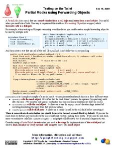
Operational Semantics We give structural operational semantics for each process term p ∈ T . The semantics is given in terms of labeled graphs with successful termination, labeled graphs for short, modulo a behavioral equivalence. A labeled graph, defined by G = (N , L, ↓, −→), has a set of nodes N , which are connected by transitions labeled by L and defined by the relation −→ ⊆ N ×L×N . Some nodes are marked by the predicate ↓ ⊆ N as having the successful termination option. For a process term p ∈ T we have a labeled graph of the form (T , A, ↓, −→), where ↓ and −→ are defined using by the structural operational rules given in Fig. 1. We will use infix a notation and write p↓ for p ∈ ↓ and p −→ p0 for (p, a, p0 ) ∈ −→. 1
2
1↓
p↓ p + q↓
3
a
5
a
a.p −→ p
6
p −→ p0 a
p + q −→ p0
q↓ p + q↓
4
a
7
q −→ q 0 a
p + q −→ q 0
p↓, q↓ p | q↓
a
8
a
p −→ p0 , q −→ q 0 a
p | q −→ p0 | q 0
Figure 1: Operational rules for the operators We briefly comment on the operational rules. Rule 1 states that the constant process 1 enables successful termination. Rules 2 and 3 show that if one component of the alternative composition has a termination option, then the alternative composition has a termination option 5
Process Algebra
as well. Rule 4 states that the synchronous parallel composition has a termination option only if both components have a termination option. Rule 5 states that action prefixes induce outgoing transitions with the same label. Rules 6 and 7 enable a nondeterministic choice between the alternatives of the parallel composition. Rule 8 states that in a synchronous parallel composition both components execute in lock-step always executing the same actions. a
a
We use the predicates p −→ and p −→ Y to denote that p has or does not have an outgoing π transition labeled by a, respectively. Let π = a1 a2 . . . an ∈ A∗ . By p −� p0 , we denote that a1 a2 a3 an p0 for some trace there exist p1 , p2 , . . . , pn−1 ∈ T such that p −→ p1 −→ p2 −→ . . . pn−1 −→ ∗ (path) π = a1 a2 . . . an ∈ A . Standardly, by ε we denote the empty trace and by π1 π2 we denote the concatenation of the traces π1 , π2 ∈ A∗ . By T(p) we denote the set of traces of p, π i.e., T(p) = {π | p−�}. 2.3
Partial Bisimilarity In this section we revisit the notion of the partial bisimilarity preorder of [28] and we show that it is a precongruence for the given operations. Definition 2.2. Let R be a relation on T . Then R is a partial bisimulation with respect to the bisimulation set B if for all p, q ∈ T such that (p, q) ∈ R the following holds: 1. if p↓, then q↓; a
a
b
b
2. for all p0 ∈ T and a ∈ A such that p −→ p0 , there exists q 0 ∈ T such that q −→ q 0 and (p0 , q 0 ) ∈ R; and 3. for all q 0 ∈ T and b ∈ B such that q −→ q 0 , there exists p0 ∈ T such that p −→ p0 and (p0 , q 0 ) ∈ R. We say that the process term p is partially bisimilar to q with respect to the bisimulation set B, notation p �B q, if there exists a partial bisimulation R with respect to B such that (p, q) ∈ R. If p �B q and q �B p, then we say that p and q are mutually partially bisimilar (with respect to B) and we write p ↔B q. When clear from the context, we will omit B. It can be easily shown that partial bisimilarity is a preorder relation [28]. Also, it is not difficult to prove that mutual partial bisimilarity is an equivalence relation [28]. Note that if the bisimulation set B is empty, i.e., B = ∅, then the partial bisimilarity preorder coincides with the standard (strong) similarity preorder and the partial bisimilarity equivalence coincides with standard similarity equivalence [14, 12]. When B = A, the partial bisimilarity preorder becomes strong bisimilarity provided that condition 1. is strengthened to “p↓ if and only if q↓", whereas mutual partial bisimilarity always turns into standard (strong) bisimilarity [14, 2]. We have the following property that characterizes the dependence on the bisimulation set B. Theorem 2.3. If p �B q, then p �C q for every C ⊆ B. Proof. Straightforward from Definition 2.2 as condition 3. holds for every b ∈ C as it holds for b ∈ B. 6
The following property states that for two process terms to be mutually partially bisimilar with respect to B it is sufficient that partial bisimulation holds in one direction and simulation in the other. Theorem 2.4. If p �B q and q �∅ p, then p ↔B q for all p, q ∈ T and B ⊆ A. Proof. Let R1 be a partial bisimulation with respect to B such that (p, q) ∈ R1 and let R2 be a simulation such that (q, p) ∈ R2 . We will show that R = R1−1 ∩ R2 is a partial bisimulation with respect to B. It is clear that (q, p) ∈ R. Suppose that (r, s) ∈ R. Then, (r, s) ∈ R1 and (s, r) ∈ R2 . Suppose that s↓. Since (s, r) ∈ R2 , we have that r↓. Suppose that there exist s0 ∈ T and a a a ∈ A are such that s −→ s0 . Then, there exists r0 such that r −→ r0 and (s0 , r0 ) ∈ R2 . a a 0 000 000 As r −→ r and (r, s) ∈ R1 , there exists s such that s −→ s and (r0 , s000 ) ∈ R1 . We a a repeat this process finitely many times coming to rˆ and sˆ such that r −→ rˆ and s −→ sˆ with b
(ˆ r, sˆ) ∈ R1 and (ˆ s, rˆ) ∈ R2 implying that (ˆ s, rˆ) ∈ R. The case when r −→ r0 for some b ∈ B is analogous. The following theorem states that partial bisimilarity �B is a precongruence with respect to the prefix, alternative composition, and synchronization operations. Theorem 2.5. Let p, q ∈ T and suppose p �B q for some B ⊆ A. Then: • a.p �B a.q, for all a ∈ A. • p + r �B q + r and r + p �B r + q , for all r ∈ T . • p | r �B q | r and r | p �B r | q, for all r ∈ T . Proof. Suppose p � q. Then there exists a partial bisimulation relation R such that pRq as given by Definition 2.2. We define for each case a separate partial bisimulation relation R0 based on R. We only show one of the symmetrical cases for the alternative and parallel composition, as the other holds by symmetry of the operational rules. • Define R0 = {(a.p, a.q)} ∪ R. The terms a.p and a.q cannot terminate and have the a a outgoing transitions a.p −→ p and a.q −→ q with (p, q) ∈ R. • Define R0 = {(p+r, q +r)}∪{(r, r) | r ∈ T }∪R. The relation R00 = {(r, r) | r ∈ T } is a partial bisimulation relation. The term p + r terminates due to a termination options of p or due to a termination option of r. In the former situation q + r terminates due to a termination option of q and in the latter due to a termination option of r. After the initial transition, the remaining terms are related by R00 , if r is chosen, or by R, if p and q are chosen. • Define R0 = {(p | r, q | r) | (p, q) ∈ R, r ∈ T }. The terms p | r and q | r either have termination options due to coinciding termination of p, q, and r or do not terminate. a a According to the operational semantics p | r−→ only if p−→ for some a ∈ A. As (p, q) are related by R, it follows directly that R0 is a partial bisimulation relation.
We have the following immediate corollary by taking into account Definition 2.2. 7
Process Algebra
Corollary 2.6. Partial bisimilarity ↔ is a congruence for T with respect to the operators a._ for a ∈ A, _ + _, and _ | _. Theorem 2.5 and Corollary 2.6 provide for substitution rules in the equational reasoning. Now, we can build the standard term model [2] for the process algebra BSP| (A, B) by using partial bisimilarity as the underlying behavioral congruence. Definition 2.7. The term algebra P(BSP| (A, B)) is given by P(BSP| (A, B)) = (T , 0, 1, a._ for a ∈ A, _ + _, _ | _). The term model of BSP| (A, B) is given by the quotient algebra P(BSP| (A, B))/↔ . 2.4
Axiomatization We give a sound and ground-complete axiomatization of the precongruence �. When we write p = q we mean that the axioms p ≤ q and q ≤ p are both included in the axiomatization. The axiomatization is given in Fig. 2. p+q=q+p p+p=p p|q=q |p 1|1=1 a.p | a.q = a.(p | q) (p + q) | r = p | r + q | r p≤p+1
A1 A3 S1 S3 S5 S7 P1
(p + q) + r = p + (q + r) p+0=p 0|p=0 1 | a.q = 0 a.p | b.q = 0, if a 6= b
A2 A6 S2 S4 S6
q ≤ a.p + q,
P2
if a 6∈ B
Figure 2: Axiomatization of � over T We briefly comment on the axioms. We note that the numbering of the axioms follows [2]. Axioms A1 and A2 express commutativity and associativity of the alternative composition, respectively. Axiom A3 shows that the alternative composition is idempotent. Axiom A6 states that deadlock does not contribute to any behavior. Axiom S1 shows that the parallel composition is commutative. Deadlock cannot synchronize with any process as expressed by axiom S2. Axioms S3 and S4 state that the successful termination option persists only if it is enabled by both processes. Axiom S5 states that processes with the same prefix synchronize, whereas axiom S6 states that no synchronization is possible between processes with different prefixes. The distribution law of the synchronous parallel composition with respect to the alternative composition is stated by axiom S7. Axiom P1 enables elimination of the successful termination option for partially bisimulated terms. Axiom P2 enables elimination of terms that are prefixed by actions that do not have to be bisimulated. We note that when the bisimulation set B = ∅ axiom P2 is valid for every possible prefix, effectively replacing axioms P1 and P2 with q ≤∅ p + q. Thus, BSP| (A, ∅) reduces to the sound and ground-complete process theory for standard similarity preorder [14, 12]. When B = A axiom P2 becomes inapplicable, as there are no actions in ∅ = A \ B. Then, the remaining axioms minus axiom P1, which allows elimination of the successful termination option, form a sound and ground-complete process theory for standard bisimulation [2, 14] of a process algebra with action prefix, alternative composition, and synchronous parallel composition. The following theorem states the axiomatization is sound and ground-complete for the partial bisimilarity preorder. 8
Theorem 2.8. The axioms of BSP| (A, B) given in Fig. 2 are sound and ground-complete for partial bisimilarity, i.e., p ≤B q is derivable if and only if p �B q. Proof. Axioms A1, A2, A3, A6, S1, S2, S3, S4, S5, S6, and S7 make a sound and groundcomplete axiomatization for strong bisimilarity, i.e., for ≤A [2]. Thus, from now on, we can assume that B 6= A. The soundness of axioms P1 and P2 follows directly by application of the operational rules and Definition 2.2 for partial bisimilarity. It is sufficient to take R = {(p, p + 1)} ∪ {(p, p) | p ∈ T } and R0 = {(q, a.p + q)} ∪ {(q, q) | q ∈ T } as partial bisimulations between the terms for axiom P1 and P2, respectively. For axiom P1 it is clear that p + 1 terminates if p c terminates and they have the same outgoing labeled transitions. For axiom P2, if q −→ q 0 for c 0 0 0 0 some q ∈ T and c ∈ A, a.p + q −→ q and (q , q ) ∈ R. Vice versa, the outgoing transitions labeled by b ∈ B of a.p + q must originate from q as a.p has only one outgoing transition b
b
labeled by a 6∈ B. Therefore, if a.p + q −→ q 0 for some q 0 ∈ T and b ∈ B, then q −→ q 0 and (q 0 , q 0 ) ∈ R. In order to show ground-completeness, we turn to normal forms as outlined, e.g., in [1, 2]. By using the axioms (for strong bisimilarity) every term p ∈ T can be rewritten as p =A P i∈I ai .pi [+1], where ai ∈ A and pi ∈ T for i ∈ I, and [+1] denotes successful termination as an optional summand [2]. Now, suppose the normal forms of p and q are: X p =A ai .pi [ + 1] and i∈I
q =A
X
cj .qj [ + 1],
j∈J
where ai , cj ∈ A \ B and pi , qj ∈ T , for i ∈ I and j ∈ J. We denote the normal forms of p and q by p0 and q 0 , respectively. From p ↔A p0 and Theorem 2.3 it follows that p ↔B p0 . Analogously, we have q ↔B q 0 , so we can conclude that p0 �B q 0 if and only if p �B q. We note that there are no idempotent summands in the normal forms. Now, the proof can be performed using induction on the total number of symbols, i.e., constants and action prefixes, of the terms. The base cases are p0 =B 0 ≤B 0 =B q 0 and p0 =B 1 ≤B 1 =B q 0 , which hold directly by using the substitution rules in an empty context, and p0 =B 0 ≤B 1 =B q 0 , which is obtained by applying 0 ≤B 0 + 1 =B 1. As p0 �B q 0 , there exists a partial bisimulation R such that (p0 , q 0 ) ∈ R. It is clear that if p0 contains the optional summand 1, then q 0 contains it as well. If q 0 comprises the summand 1 and a p0 does not contain it, then we use axiom P1 to eliminate it. Suppose that p0 −→ p00 for some 00 a ∈ A and p ∈ T . Then, according to the operational rules there exists a summand ak .pk of p0 for some k ∈ I such that ak = a and pk = p00 . Analogously, by Definition 2.2 there exists a summand c` .q` of q 0 , such that c` = a and (pk , q` ) ∈ R for some ` ∈ J. So, pk �B q` and, hence, by the induction hypothesis, pk ≤B q` . Thus, there exists L ⊆ J such that for every i ∈ I there exists ` ∈ L such that ai .pi ≤B c` .q` . Vice versa, for every j ∈ J such that cj ∈ B there exists k ∈ I such that ak .pk ≤B cj .qj . Denote by K = L ∪ {j | cj ∈ B, j ∈ J}. Now, we split q 0 to q 0 = q 00 + q 000 such that q 00 000 contains the summands that are prefixed by an action P in B or that have an Pindex in L and q comprises the remaining summands, i.e., q 00 = k∈K ck .qk and q 000 = `∈J\K c` .q` . Note that p000 contains only summands prefixed by actions that are not in B. Now, we have that p =B p0 ≤B q 00 . By applying Axiom P2 for the summands c` .q` of q 000 for ` ∈ J \ K we obtain q 00 ≤B q 00 + q 000 =B q 0 =B q, leading to p ≤B q, which completes the proof. 9
Process Algebra
We conjecture that the partial bisimilarity equivalence does not admit a finite axiomatization when ∅ ⊂ B ⊂ A. To illustrate this, we consider the set of equations E = {a.bn .0 + a.bn .a.0 =B a.bn .a.0 | a 6∈ B, b ∈ B, n ∈ N}, where bn .p is defined recursively as b0 .p , p and bn+1 .p , b.bn .p. It is not difficult to check that a.bn .0 + a.bn .a.0 ↔B a.bn .a.0 for every n ∈ N. However at depth greater than 1, we have b.p + b.q ↔B b.q, which holds only when p ↔B q, which is not the case for p , bn .0 and q , bn .a.0. This insinuates that E is a set of axioms. In the literature the summand a.bn .0 is also known as the ‘little brother summand’ of a.bn .a.0. Little brother summands occur when dealing with similarity-like equivalences and have a very important role in their characterization [7, 13, 5]. Two similar terms that do not contain little brother summands are actually strongly bisimilar. This claim holds immediately for partial bisimilarity as well, having in mind Theorem 2.3. Definition 2.9. Let p =B a.p0 + a.p00 + p000 for some a ∈ A such that a.p0 ≤B a.p00 holds, but a.p00 ≤B a.p0 does not hold. Then, we say that a.p0 is the little brother of a.p00 . The following properties show the nature of mutual partial bisimilarity. Theorem 2.10. Suppose that p ≤ q ≤ r. Then, the following equations hold: if a 6∈ B
a.p + a.q = a.q
P3
b.p + b.q + b.r = b.p + b.r
if b ∈ B
P4.
Proof. We show that the equations are sound by showing the inequalities in both directions. For equation P3 we have that a.p+a.q≤a.p holds directly by axiom P2. For the other direction we calculate a.p = a.p + a.p ≤ a.p + a.q using axiom A3 and the premise, respectively. For equation P4 we have the following derivation, calculated by using axiom A3 and the premise, accordingly: b.p + b.q + b.r ≤ b.p + b.r + b.r = b.p + b.r b.p + b.r = b.p + b.p + b.r ≤ b.p + b.q + b.r, which completes the proof. These equations show how to eliminate little brother summands. We note that idempotency of the alternative composition, given by axiom A3, is used in the situation when p≤q and q≤p, even though we do not distinguish this in the conditions of the equations above. Equation P3 is actually a more general form of the known characteristic equation of the (strong) similarity equivalence stated in the form a.(p + q) + a.q = a.(p + q) in [14]. As for strong similarity the prefix action does not play any role the axiom is always applicable. To establish partial bisimilarity when the little brothers are prefixed by an action in the bisimulation set B, the ‘littlest’ and the ‘biggest’ brother must be preserved. The equations given by Theorem 2.10 set the rules for elimination of little brothers when deriving the minimal mutual partially bisimilar quotient. 2.5
Modal Characterization We give a modal characterization of the partial bisimilarity preorder in the vein of [14]. The following definition gives the partial bisimilarity formulas. Definition 2.11. The partial bisimilarity modal formulas are given by F defined as follows: N ::= > | ¬> | ¬1 | ¬haiF | ¬(F ∧ F ) | hbiN F ::= > | ¬> | 1 | haiF | F ∧ F | ¬N,
10
where a ∈ A and b ∈ B. The set of all partial bisimilarity modal formulas with respect to a bisimulation set B is denoted by F(B). The satisfaction relation |=⊆ T × F(B) is defined recursively by: • p |= > for all p ∈ T ; • p |= 1 if and only if p↓; a
• p |= haif if there exists p0 ∈ T such that p −→ p0 and p0 |= f ; • p |= ¬f if not p |= f ; • p |= f ∧ g if p |= f and p |= g. Note that formulas given by N are negations of formulas defined by F . It preserves that the negation, which characterizes bisimilar behavior, is enabled only for actions in the bisimulation set B. The partial bisimilarity modal formulas are a superset of the modal formulas for similarity and a subset of the ones for bisimilarity because negation is not present in the former and allowed for all formulas in the latter. When B = ∅, the modal formulas given by F minus the successful termination predicate 1 reduce to the ones for similarity [14], i.e., F reduces to F ::= > | ¬> | haiF | F ∧ F . When B = A and, again, provided that we ignore the termination predicate 1, F reduces to F ::= > | haiF | F ∧ F | ¬F , i.e., the Hennessy-Milner formulas over A that identify bisimulation [14]. The following theorem shows that a process p is partially bisimilar to a process q if and only if all partial bisimilarity modal formulas that are satisfied by p are also satisfied by q. Theorem 2.12. Let p, q ∈ T . Then, p �B q if and only if for every f ∈ F(B) it holds that if p |= f then q |= f . Proof. First we show the implication from left to right. Suppose that p �B q and p |= f for some f ∈ F(B). We will show that q |= f by structural induction on f . • Suppose f ≡ 1. According to Definition 2.11 p↓. As p �B q, we have that q↓. Thus, q |= 1. a
a
• Suppose f ≡ haif 0 . Then p −→ p0 with p0 |= f 0 . We have that q −→ q 0 and p0 �B q 0 . By the hypothesis q 0 |= f 0 and, thus, q |= f . b
• Suppose f ≡ ¬hbif 0 . Then for all p0 ∈ T such that p −→ p0 , it holds p0 |= ¬f 0 . Note b
b
that ¬f 0 ∈ F(B). As p �B q, we have that q −→ . Suppose that q −→ q 0 . We will show that q 0 |= ¬f 0 by contradiction. Suppose that q 0 |= f 0 . Then, there exists p00 ∈ T such b
that p −→ p00 . From above, p00 |= ¬f 0 , so by the hypothesis q |= ¬f 0 , which leads to contradiction. Thus, q 0 |= ¬f 0 implying that q |= f . • Suppose f ≡ f 0 ∧ f 00 . Then p |= f 0 and p |= f 00 implying that q |= f 0 and q |= f 00 by the induction hypothesis, so q |= f . Next, we show the implication to left. Suppose that for every f ∈ F such that p |= f it holds q |= f as well. We will show that there exists a partial bisimulation by induction on the number of constants and action prefixes in p. The base cases are: (1) If p ≡ 0, then p |= ¬hbi> for all b ∈ B are all non-trivial formulas b
satisfied by p leading to q |= ¬hbi>. So, q −→ Y implying p �B q. (2) If p ≡ 1, then we have (1) and p |= 1 implying that q |= 1. So, p↓ implies that q↓. 11
Process Algebra
a
Now, suppose that p↓. Then p |= 1, so q |= 1 as well, implying q↓. Suppose that p −→ p0 and a p0 |= f 0 . Then, p |= haif 0 , so q |= haif 0 , i.e., q −→q 0 and q 0 |= f 0 . By the induction hypothesis b
we have that p0 �B q 0 . Finally, suppose that q −→ q 0 and q 0 |= f 0 for some f 0 ∈ F. We will b
b
show that p −→ p0 and p0 �B q 0 by contradiction. It must be that p−→ because in the opposite b
case p |= ¬hbi> implying q |= ¬hbi> which leads to contradiction. Suppose that p −→ p0 and p0 |= ¬f 0 . Note that it must be that ¬f 0 ∈ F. Then, p |= ¬hbif 0 , implying that q |= ¬hbif 0 . b
So, we have that for all q 0 such that q −→ q 0 it holds that q 0 |= ¬f 0 leading to contradiction. Thus, p0 |= f 0 , so p0 �B q 0 implying that p �B q, which completes the proof. 2.6
Recursion We introduce recursion by means of guarded essentially finite state recursive specifications, which induce finite state transition systems [3] to obtain BSP| (A, B, R), where R is the set of recursion variables. We restrict only to such specifications as every finite state transition system can be specified as a guarded essentially finite state recursive specification [3]. The restriction is given by forcing seriality of recursive variables [3], i.e., no free occurrence of a recursive variable is in the scope of the parallel composition, as well as requiring that they are guarded, i.e., every recursive variable is encapsulated by the action prefix operator. Processes given as solutions to the recursive specifications have the following signature: µX.{X = G | X ∈ R, R ⊆ R}, which is added to the existing signature of the process algebra, where G ::= P | a.T | G + G,
T ::= X | G | T + T,
and P is given by Definition 2.1. We will denote the set of guarded essentially finite state recursive specifications by S. Before we introduce the standard operational rules, we give a useful notation [2]. By tX we will denote the term defining variable X. Also, we generalize µX.S, for S ∈ S, to µp.S, for p ∈ T using the following inductive definition: Definition 2.13. Define µpS, for p ∈ T and S ∈ S, using structural induction, as follows: µ0.S = 0 µ1.S = 1 µ(a.q).S = a.(µq.S) µ(q + r).S = µq.S + µr.S µ(µX.S).S = µX.S Note that in p all free occurrences of X are replaced by µX.S. Now, the standard operational rules for solutions of recursive specifications can be stated as given in Fig. 3.
9
µtX .S ↓ µX.S ↓
a
10
µtX .S −→ p a
µX.S −→ p
Figure 3: Operational rules for the solutions of the recursive specifications
The axioms in Fig. 4 capture the recursive definition and recursive specification principles, 12
which state that every recursive specification has a solution and that the guarded recursive specifications have at most one solution [3, 2]. µX.S ] {Y = tY } = µ(µX.S).{Y = tY }
if X 6= Y
A1
µX.{X = t} = µt.{X = t}
A2
if t{p/X} ≤ p then µX.{X = t} ≤ p
A3
if p ≤ t{p/X} then p ≤ µX.{X = t}
A4
Figure 4: Axioms for manipulation with recursive specifications Axiom A1 enables decomposition of the recursive specification to only one equation. This provides for head normal forms which contain only recursive specification of the form µX.X = t [3]. Axiom A2 is the standard unfolding axiom, recall Definition 2.13 for the extended syntax. Axioms A3 and A4 are the folding axioms, which originate from [12], where it is shown that they hold for simulation. The combination of axioms A3 and A4 gives rise to the standard folding axiom if t{p/X} = p then µX.{X = t} = p. Next, we develop a partitioning algorithm for computing the mutual partial bisimilarity quotient.
3 Controllability We define controllability from a process algebraic perspective in terms of partial bisimilarity preorder. Standardly, we split A into a set of uncontrollable actions U ⊆ A, and a set of controllable actions C = A \ U. The plant, the control requirements, and the supervisor are specified as process terms, relying on BSP| (A, U). Intuitively, outgoing uncontrollable transitions of the plant should be bisimilar to the ones of the supervised plant, so that the reachable uncontrollable part of the former is indistinguishable from the one of the latter. The outgoing controllable transitions of the supervised plant may only be simulated by the ones of the original plant, since some undesired controllable transitions are suppressed by the supervisor. We use p ∈ T to denote the plant, r ∈ T for the control requirements, and s ∈ T to denote the supervisor. Consequently, the supervised plant is given by p | s. First, we introduce the control problem and, afterwards, we characterize the existence of a deterministic supervisor. Definition 3.1. Let p ∈ T be the plant and r ∈ T be the control requirements. The control problem is to find a supervisor s ∈ T such that p | s ≤U p and p | s ≤∅ r. As expected, Definition 3.1 ensures that no uncontrollable actions have been disabled in the supervised plant, by including them in the bisimulation set. Moreover, it takes into account the nondeterministic behavior of the system. It suggests that the plant is modeled as is, whereas the control requirements are modeled as desired behavior, independent of the plant. This is in contrast with much work done in this area, where the aim is to satisfy a given desired controllable behavior. Still, we opt for an ‘external’ specification in process algebraic spirit, where, e.g., one wants to show that a given protocol behaves like a buffer when abstracted from the internal protocol communication. In this context, the control requirement 13
Controllability
is the buffer, whereas the protocol is treated as a plant. Following this approach we only require that the supervised plant has a behavior that can be simulated by the control requirements. The setting described above is also a preparation for future work, where we intend to relax this condition in the vein of [29, 20], abstracting from irrelevant internal actions in the control requirements, an approach advocated from process algebraic perspective as well. Nonetheless, hiding in [29, 20] is performed in trace semantics, whereas abstraction should preserve branching behavior. Moreover, in [29, 20] the goal is to achieve bisimilarity and similarity with the control requirements, respectively, again insinuating that the control requirements are seen as the abstracted behavior of the supervised plant. The approach of [10] couples the requirements with the plant even more closely, requiring that they play the role of the supervisor as well. Note that if we assume that r represents the desired behavior of the supervised plant, then we require that r ≤U p, since r ≤∅ r, as in the original setting of [27]. When p and r are deterministic that this amounts to standard language controllability [28]. As argued above, we choose bisimilarity as an appropriate behavioral equivalence that captures nondeterminism. Therefore, one expects that when we take the plant as a control requirement, the resulting controllability conditions p | s ≤U p and p | s ≤∅ p will amount to bisimilarity. The conditions collapse to p | s ≤U p, as p | s ≤U p implies p | s ≤∅ p. Now, we can seek the largest possible supervised plant, i.e., p ≤U p | s, leading to p | s =U p. Note that the plant can have redundant behavior in the form of little brothers, which prevents a bisimilarity between p and p | s to be established. Nevertheless, under the assumption that no little brothers are present, p | s =U p implies p | s =A p, as shown in [5] for similarity equivalence, further justifying the choice of partial bisimilarity preorder. According to Definition 3.1, the minimal possible supervisor is the initial uncontrollable reach of the plant, given by the topmost subterm of p comprising only uncontrollable prefixes. For example, the minimal supervisor of p , µX.{X = u.X +c.u.X +v.c.0}, assuming that p =U r, u, v ∈ U, and c ∈ C, is the process s , µX.{X = u.X + v.0}. According to Definition 3.1, every plant becomes controllable with respect to itself, i.e., every plant can accept itself as control requirement. This is a downside of the notion of state controllability, used in the nondeterministic setting of [10, 29, 20]. As an illustration, let p =U r with p , u.v.0 + u.w.0, where u, v, w ∈ U. Then, the plant is not state controllable with respect to itself, which is directly checked using the definition from the introduction. However, a non-restricting supervisor s , µX.{X = u.X + v.X + w.X}, which enables all transitions, always exists. Another supervisor is the determinized version of the control requirements, given by s0 , u.(v.0 + w.0). As illustrated above, a usual suspect for a deterministic supervisor is the determinized version of a desired supervised behavior. First, we define a determinized version det(p) of a a a process p ∈ T . By Tar(p −→ ) , {p0 ∈ T | p −→ p0 } denote all target processes that are reachable from p ∈ T by an outgoing transition labeled by a ∈ A. The determinized version of p is defined as follows:
11
p↓ det(p)↓
a
12
p −→ P a a det(p) −→ det( p0 ∈Tar(p−→) p0 )
Rule 11 states that the original and determinized process have the same termination options. Rule 12 merges a nondeterministic choice over equally labeled transitions to a single transition which target is the alternative composition of all original target processes. It is not difficult to observe that p | det(p) =B p for all p ∈ T and B ⊆ A, as det(p) does not disable any transition of p. 14
Suppose that a desired behavior of the supervised plant is given by q ∈ T such that q ≤U p and q ≤∅ r. The control problem is to find a supervisor s ∈ T , such that p | s =U q. A good candidate is s , det(q), since from q ≤U p we have that q | det(q) ≤U p | det(q), implying q ≤U p | det(q). Now, we need a characterization when p | det(q) ≤U p, as it does not hold in general. Theorem 3.2. For all p, q ∈ T , p|det(q) ≤U p if and only if det(p)|det(q) ≤U det(p). Proof. Suppose that p | det(q) ≤U p. Then, there exists a partial bisimulation R such that t
(p | det(q), p) ∈ R. By p −� p0 denote that there exist p1 , p2 , . . . , pn−1 ∈ T such that ε a1 a2 a3 an p1 −→ p2 −→ . . . pn−1 −→ p0 for some trace t = a1 a2 . . . an ∈ A∗ with p −� p. By p −→ t
t
Tar(p −� ) , {p0 ∈ T | p −� p0 } denote the target processes P reachable from p followP ing a trace t. Now, define R0 = {(det( 0 p0 ) | q 0 , det( 0 p0 )) | (p00 | t t 0
000
∗
p ∈Tar(p−�) t
p ∈Tar(p−�)
t
00
000
q , p ) ∈ R and there exists t ∈ A such that p −� p and p −� p }. We will show that P t R0 is a partial bisimulation. Note that det(p) −� det( 0 p0 ) for every t ∈ A∗ . t p ∈Tar(p−�)
For t = ε, we have that (det(p) | det(q), det(p)) ∈ R0 . Suppose that (r0 | q 0 , r0 ) with P r0 , det( p0 ) for some t0 ∈ A∗ . If r0 | q 0 ↓ then, r0 ↓ and q 0 ↓. Suppose that t0 a
p0 ∈Tar(p−�)
a
r0 | q 0 −→ r00 | q 00 for some a ∈ A and r00 , q 00 ∈ T . Then, r0 −→ r00 and there exist p01 , q10 ∈ T t
t
a
a
such that p −� p01 and q −� q10 with p01 −→ p02 and q10 −→ q20 . Note that q10 is uniquely det
a
termined. Then, (p01 | q10 , p001 ) ∈ R for some p001 ∈ T such that p −� p001 and p001 −→ p002 with b
(p02 | q20 , p002 ) ∈ R, implying that (r00 | q 00 , r00 ) ∈ R0 . The proof when r0 −→ r00 for some b ∈ B and r00 ∈ T is analogous. Suppose that det(p)|det(q)≤U det(p). Then there exists a partial bisimulation relation R such t
t
that (det(p)|det(q), det(p)) ∈ R. Define R0 = {(p0 | q 0 , p0 ) | p −� p0 , det(q) −� q 0 and (p00 | t
q 0 , p00 ) ∈ R where det(p) −� p00 for t ∈ A∗ }. Then, R0 is a partial bisimulation relating p | det(q) and p. The proof follows the same lines as above. Relying on Theorem 3.2 and Theorem 2.4, we characterize when desired behavior given by q ∈ T is controllable with respect to plant p ∈ T and control requirements r ∈ T . Definition 3.3. Process q ∈ T is controllable with respect to plant p ∈ T and control requirements r ∈ T , a if q ≤U p, p | det(q) ≤∅ r, det(q) ≤U det(p), and p | det(q) ≤∅ q. The definition requires that (1) the plant partially bisimulated and the requirements simulate the behavior of the supervised plant, so that Definition 3.1 is satisfied, i.e., it is ensured that the supervised behavior satisfies the requirements and it is compatible with the plant on the uncontrollable events; (2) the deterministic behavior of the supervised plant, i.e., its language, is partially bisimulated by the plant, implying that the deterministic version of the desired behavior of the supervised plant can be used as a supervisor; and (3) the supervised behavior should simulate the supervised plant, implying that they are mutually partially bisimilar. We note that if equivalence is not desired, i.e., the supervised plant should only contain the desired behavior, then we can eliminate the third condition. The following theorem states the existence of a supervisor. Theorem 3.4. If q ∈ T is controllable with respect to a plant p ∈ T and control requirements r ∈ T , then det(q) is a supervisor for p with respect to r. 15
Controllability
Proof. From det(q) ≤U det(p) and Theorem 3.2 we have that p | det(q) ≤U p. Then, from p | det(q) ≤∅ q and Theorem 2.4 we have that p | det(q) =U q. Finally, from q ≤U p and q ≤∅ r we have that p | det(q) ≤U p and p | det(q) ≤∅ r, which completes the proof.
We note that the minimal deterministic supervisor of the plant p such that the supervised plant contains the behavior of q, i.e., q ≤U p, is det(q). So, for any other supervisor s ∈ T that satisfies the above relation, we must have that q ≤∅ s and det(p)|det(s) ≤U det(p). We can also demand that the control requirements r are controllable, i.e., we wish that the desired behavior of the plant is the same as the control requirement. This amounts to r ≤U p, det(r) ≤U det(p), and p | det(r) ≤∅ r. It is directly observed that the first requirements ensured compatibility of the control requirements with the plant, the second requirement is equivalent to language controllability, whereas the third requirement induces a refinement relation of the behavior of the supervised and the control requirements, respectively, comparable to the approaches of [23, 29, 20]. We note that for deterministic systems, we the first and the second condition coincide. The requirements can be efficiently checked using the algorithm presented in the following section. Finally, note that the plant p can be replaced by any p0 such that p0 =U p, providing for a minimization procedure that preserves controllability.
4 Partial Bisimulation Algorithm We give a partitioning algorithm for computing the mutual partial bisimilarity quotient of a given labeled graph. With small adjustments the algorithm can be used to check whether two labeled graphs are partially bisimilar, as for the similarity equivalence [13]. The algorithm exploits the idea that partial bisimilarity equivalence can be presented as a partition pair, as it was done for the similarity equivalence in [13, 26]. The algorithm presented in [13] was mended in [15]. An extended version with proofs concerning the stability conditions for similarity can be found in [26]. We improve upon these works by employing the efficient splitting technique of [24, 11]. N Let S G = (N , L, ↓, −→) be a labeled graph. A set P is a partition over N if P ⊂ 2 such that P ∈P P = N and for all P, Q ∈ P if P ∩ Q 6= ∅, then P = Q. A partition pair over G is a pair (P, v) where P is a partition over N and the (little brother) relation v ⊆ P × P is a partial order, i.e., a reflexive, antisymmetric, transitive relation. We note that our definition is stronger in the sense that we require v to be antisymmetric and transitive, opposed to only acyclic as originally defined in [13].
For all P ∈ P, by P ↓ and P 6 ↓ we denote that p↓ and p6 ↓, respectively, for all p ∈ P . For a a P 0 ∈ P by p −→ P 0 we denote that there exists p0 ∈ P 0 such that p −→ p0 . We distinguish two a types of (Galois) transitions between the partition classes [13, 16]: P −→∃ P 0 , which denotes a a that there exists p ∈ P such that p −→ P 0 , and P −→∀ P 0 , which denotes that for every a a a p ∈ P it holds that p −→ P 0 . It is straightforward that P −→∀ P 0 implies P −→∃ P 0 . Also, if a a a a 0 0 Y ∃ P and p −→ Y ∀ P we denote that there P −→∀ P , then Q −→∀ P for every Q ⊆ P . By p −→ a a are no transitions p −→∃ P and p −→ Y ∀ P , respectively. The following definition gives the stability conditions for partial bisimilarity of a partition pair with respect to the termination predicate and the transition relation. Definition 4.1. Let G = (N , L, ↓, −→) be a labeled graph. We say that a partition pair (P, v) over G is stable with respect to B, ↓, and −→ if the following conditions are fulfilled: 16
a. For all P ∈ P it holds that P ↓ or P 6 ↓. b. For all P, Q ∈ P such that P v Q if P ↓, then Q↓. a
c. For every P, Q, P 0 ∈ P and a ∈ A such that P v Q and P −→∃ P 0 there exists Q0 ∈ P a such that P 0 v Q0 and Q −→∀ Q0 . b
d. For every P, Q, Q0 ∈ P and b ∈ B such that P v Q and Q −→∃ Q0 there exists a P such b
that P v Q and P −→∀ P 0 . Note that when B = A, from P v Q we can straightforwardly deduce that Q v P by interchanging stability conditions c and d. Therefore, stability conditions c and d become: for a a every P ∈ P and a ∈ A, if P −→∃ P 0 , then P −→∀ P 0 , which is the stability condition for the bisimulation equivalence [11]. When B = ∅, stability condition d is inapplicable, whereas stability condition c is the stability condition for the simulation preorder [13, 26]. Given a relation R ∈ S × T , define R−1 ∈ T × S as R−1 = {(t, s) | (s, t) ∈ R}. If R is a preorder, then R ∩ R−1 is an equivalence relation. The following theorem shows that every partial bisimulation preorder induces a stable partition pair. Theorem 4.2. Let G = (N , A, ↓, −→) with N ⊂ T and let R be a partial bisimulation preorder over N with respect to B. Let ↔ , R ∩ R−1 . If P = T /↔ and for all p, q ∈ N it holds if (p, q) ∈ R, then [p]↔ v [q]↔ , then the partition pair (P, v) is stable with respect to B, ↓, and −→. Proof. Let P = [p]↔ , P 0 = [p0 ]↔ , P 00 = [p00 ]↔ , Q = [q]↔ , Q0 = [q 0 ]↔ , and Q00 = [q 00 ]↔ for p, p0 , p00 , q, q 0 , q 00 ∈ N . First, we show that v is a partial order. Reflexivity holds as for all p0 ∈ [p]↔ it holds that (p, p0 ) ∈ R implying P v P . To show antisymmetry, suppose that P v Q and Q v P . Then (p, q) ∈ R and (q, p) ∈ R, implying (q, p), (p, q) ∈ R−1 and P = Q. Finally, suppose that P v P 0 and P 0 v P 00 . Then (p, p0 ), (p0 , p00 ) ∈ R. As R is a preorder, we have (p, p00 ) ∈ R implying that P v P 00 . So, (P, v) is a partition pair. Next, we show that the stability conditions of Definition 4.1 hold. 1. Suppose that p↓. For every p0 ∈ [p]↔ it holds that p ↔ p0 , so p0 ↓ implying P ↓. Analogously for p6 ↓. 2. Let P, Q ∈ P be such that P v Q. Now, if P ↓, then p↓, which implies that q↓ and also Q↓. a
3. Suppose that P v Q and P −→∃ P 0 . Then, there exist p ∈ P and p0 ∈ P 0 such that a a p −→ p0 . As (p, q) ∈ R and v is a partial order, there exists Q0 ∈ P such that q −→ q 0 a and (p0 , q 0 ) ∈ R, and for all q 000 ∈ N if q −→ q 000 and (p0 , q 000 ) ∈ R then Q000 v Q0 or ¯ 0 such Q000 and Q0 are unrelated. Now, let q¯ ∈ Q. As (q, q¯) ∈ R there exists q¯0 ∈ Q a 0 0 0 0 0 00 ¯ that q¯ −→ q¯ and (q , q¯ ) ∈ R. Then Q v Q . As (¯ q , q) ∈ R then exists q ∈ Q00 such a 00 0 00 0 0 00 ¯ ¯ 0 = Q00 . Thus, that q −→ q and (¯ q , q ). Then Q v Q v Q implying that Q0 = Q a Q −→∀ Q0 . b
4. Suppose that P v Q and Q −→∃ Q0 . The proof that there exists P 0 v Q0 such that b P −→∀ P 0 is analogous to 2.
17
Partial Bisimulation Algorithm
Vice versa, every stable partition pair induces a partial bisimulation preorder. Theorem 4.3. Let G = (N , A, ↓, −→) with N ⊂ T and let (P, v) be a partition pair. Define R = {(p, q) | P v Q, p ∈ P, q ∈ Q}. If (P, v) is stable with respect to B, ↓, and −→, then R is a partial bisimulation preorder. Proof. Let P = [p]↔ , P 0 = [p0 ]↔ , P 00 = [p00 ]↔ , Q = [q]↔ , Q0 = [q 0 ]↔ , and Q00 = [q 00 ]↔ for p, p0 , p00 , q, q 0 , q 00 ∈ N . Suppose (p, q) ∈ R. In that case P v Q. We will show that the stability conditions of Definition 2.2 hold for R. 1. If p↓, then P ↓. So, Q↓ implying q↓. a
a
2. Suppose p −→ p0 for some a ∈ A. Then, P −→∃ P 0 implying that there exists Q0 ∈ P a a such that Q −→∀ Q0 . It follows that there exists q 0 such that q −→ q 0 and (p0 , q 0 ) ∈ R. b
b
3. Suppose q −→ q 0 for some b ∈ B. Then, Q −→∃ Q0 implying that there exists P 0 ∈ P b
b
such that P −→∀ P 0 . It follows that there exists p0 such that p −→ p0 and (p0 , q 0 ) ∈ R.
Next, lets us define a partial order C on the partition pairs as follows. Definition 4.4. Let (P, v) and (P 0 , v0 ) be partition pairs. We say that (P, v) is finer than (P 0 , v0 ), notation (P, v) C (P 0 , v0 ), if and only if for all P, Q such that P v Q there exist P 0 , Q0 ∈ P 0 such that P ⊆ P 0 , Q ⊆ Q0 , and P 0 v0 Q0 . Now, it is not difficult to observe that finding the C-maximal stable partition pair over a labeled graph G coincides with the problem of finding the coarsest partial bisimulation preorder over G. This is expressed by the following theorem. Theorem 4.5. Let G = (N , A, ↓, −→) with N ⊂ T . The C-maximal partition pair (P, v) stable with respect to B, ↓, and −→ is induced by the partial bisimilarity preorder �B , i.e., P = N /↔B and [p]↔B v [q]↔B if and only if p �B q. Proof. By Theorem 4.2, the partition pair (P, v) is stable with respect to B, ↓, and −→. Suppose that (P 0 , v0 ) is another partition pair that is stable with respect to B, ↓, and −→. Then by Theorem 4.3 it induces a partial bisimulation preorder R0 with respect to B. It is straightforward that R0 ⊆ �B . We will show that (P 0 , v0 ) C (P, v). Suppose that P 0 v0 Q0 for some P 0 , Q0 ∈ P 0 . Let p0 ∈ P 0 and q 0 ∈ Q0 . Then, (p0 , q 0 ) ∈ R0 , implying that p0 �B q 0 . It follows that [p0 ]↔B v [q 0 ]↔B , which completes the proof. The algorithm iteratively refines the partition pair (P00 , v00 ) = ({N }, {(N , N )}) over G = (N , A, ↓, −→) until it reaches the C-maximal stable partition pair. We refine the partition by choosing splitters, which represent subsets of nodes that do not adhere to the stability conditions in combination with other nodes from the same class and, therefore, must be placed in a separate class. This induces a refinement of the partition, since a larger class, referred to as parent, is split into two or more classes. We manipulate with the splitters in the vein of [24, 11], which optimizes the computation of the refinements. For that reason, we need an initial set of splitters, which is computed according to the termination options and the outgoing labeled transitions of the states as follows. 18
Condition a of Definition 4.1 requires that all states in a class have or, alternatively, do not have termination options. Thus, we can immediately split N to P0 and P1 such that P0 ↓ and P1 6 ↓ with P0 v P1 . Note that at this point the relation v denotes the potential of P0 being the little brother of P1 . We are certain that P1 v P0 is not possible for any refinement of the partition {P0 , P1 } because of stability condition b of Definition 4.1. Moreover, as any further refinement will actually refine (P00 , v00 ) , ({P0 , P1 }, {(P0 , P0 ), (P0 , P1 ), (P1 , P1 )} stability conditions a and b will always be satisfied, so we no longer have to take them into a consideration during refinement. Next, let the set of outgoing labels OL(p) , {a ∈ A | p−→} denote the set of labels of all outgoing transitions of the node p ∈ N . We refine (P00 , v00 ) as follows. Suppose that the partition pair (P0 , v0 ) such that (P0 , v0 ) C (P00 , v00 ) is the desired partition pair of splitters. The partition P0 is defined as for every P ∈ P0 , p, q ∈ P if and only if OL(p) = OL(q), since if p and q do not have the same sets of outgoing labels, then they cannot be mutually partially bisimilar. This induces the sets OL(P ) , OL(p) with p ∈ P . We define the little brother relation by looking into the sets of outgoing labels. Recall that partially bisimilar terms must have the same sets of outgoing labels that are also in the bisimulation set. The set of remaining outgoing labels of the little brother, which transitions only have to be simulated, is a subset of the corresponding set of outgoing labels of the other term. So, we put P v0 Q if and only if (1) OL(P ) \ B ⊆ OL(Q) \ B, and (2) OL(P ) ∩ B = OL(Q) ∩ B. As (P0 , v0 ) C (P00 , v00 ), we have that if P ∈ P1 then Q ∈ P1 . The initial little brother relation v0 satisfies the conditions of Definition 4.1, i.e., it is a partial order. It is easily observed that the stability conditions are not necessarily satisfied for (P0 , v0 ). However, if we consider (P0 , v0 ) with respect to the partition pair (P00 , v00 ) we see that the stability conditions are satisfied. For example, for all P, Q ∈ P0 , P 0 ∈ P00 , and a ∈ A it a a holds that if P −→ P 0 , then there exists Q0 ∈ P00 such that P 0 v Q0 and Q −→ Q0 . It is clear 0 0 that (P0 , v0 ) C (P0 , v0 ). Now, the idea behind the partitioning algorithm is to iteratively refine (P00 , v00 ) to (Pn0 , v0n ) and (P0 , v0 ) to (Pn , vn ) for some n ∈ N. For all 0 ≤ i ≤ n we have that (Pi , vi ) C (Pi0 , v0i ) and the stability conditions are satisfied for (Pi , vi ) with respect to (Pi0 , v0i ). Moreover, (Pn , vn ) and (Pn0 , v0n ) is a fix point of the algorithm, i.e., (Pn , vn ) = (Pn0 , v0n ). The refinement of (P 0 , v0 ) and (P, v) employs the splitters, which are initially formed of classes, which nodes cannot be combined as they contravene the stability conditions. The C-maximality is achieved by showing that if a splitter contains nodes from two different classes, then it is unstable, e.g., as it was done for the initial classes above, implying that the resulting partition is the coarsest possible refinement. Now, suppose that the partition pair (P, v) has (P 0 , v0 ) as parent with (P, v) C (P 0 , v0 ). For convenience, we rewrite the stability conditions c and d of Definition 4.1 for the partition pair (P, v) with respect to (P 0 , v0 ) and the bisimulation set B: a
1. For all P ∈ P, a ∈ A, and P 0 ∈ P 0 such that P −→∃ P 0 there exists Q0 ∈ P 0 such that a P 0 v0 Q0 and P −→∀ Q0 . a
2. For all P, Q ∈ P, a ∈ A, and P 0 ∈ P 0 such that P v Q and P −→∀ P 0 there exists a Q0 ∈ P 0 such that P 0 v0 Q0 and Q −→∀ Q0 . b
3. For all P ∈ P, Q0 ∈ P 0 , and b ∈ B such that P −→∃ Q0 there exists P 0 ∈ P 0 such that b
P 0 v0 Q0 and P −→∀ P 0 . b
4. For all P, Q ∈ P, Q0 ∈ P 0 , and b ∈ B such that P v Q and Q −→∀ Q0 there exists b P 0 ∈ P 0 such that P 0 v0 Q0 and P −→∀ P 0 . 19
Partial Bisimulation Algorithm
It is not difficult to observe that stability conditions 1 and 2 replace stability condition c of Definition 4.1, where as stability conditions 3 and 4 replace stability condition d of Definition 4.1. They are equivalent when (P, v) = (P 0 , v0 ). From now on, we refer to the stability conditions above instead of the ones in Definition 4.1. The form of stability conditions as given above is useful as stability conditions 1 and 3 can be used to split the classes, whereas stability conditions 2 and 4 can be used to adjust the little brother relation. We proceed in the vein of [24, 11], and we define the function cnt : N × A × 2N → N to a optimize the splitting process, where cnt(p −→ P 0 ) ≥ 0 denotes the number of transitions labeled by a ∈ A from the node p ∈ N to the parent P 0 ∈ P 0 . Suppose that we refine the partition pair (P 0 , v0 ) that is a parent of (P, v) C (P 0 , v0 ), where P 0 ∈ P 0 is such that S 0 ⊂ P 0 . The refinement step splits P 0 to S 0 and P 0 \ S 0 and subsequently splits every class in P with respect to the splitter S 0 in order to satisfy the stability conditions. If one knows a a cnt(p −→ P 0 ) and cnt(p −→ S 0 ) has been computed for every node p ∈ N and action a ∈ A, then this information can be used to update the function cnt for P 0 \ S 0 and deduce the following: a
a
a
a
a
0 0 0. If cnt(p −→P 0 ) = cnt(p −→S 0 ) = 0, then p −→S Y , p −→P Y \S 0 , and cnt(p −→P 0 \S 0 ) = 0. a
a
a
a
a
1. If cnt(p −→ P 0 ) > 0 and cnt(p −→ S 0 ) = 0, then p −→ Y S 0 , p −→ P 0 \ S 0 , and cnt(p −→ a 0 0 0 P \ S ) = cnt(p −→ P ). a
a
a
a
a
0 2. If cnt(p −→P 0 ) = cnt(p −→S 0 ) > 0, then p −→S 0 , p −→P Y \S 0 , and cnt(p −→P 0 \S 0 ) = 0. a
a
a
a
3. If cnt(p −→ P 0 ) > 0, cnt(p −→ S 0 ) > 0, and cnt(p −→ S 0 ) 6= cnt(p −→ P 0 ), then a a a a a p −→ S 0 , p −→ P 0 \ S 0 , and cnt(p −→ P 0 \ S 0 ) = cnt(p −→ P 0 ) − cnt(p −→ S 0 ). The advantage of this approach is that in order to decide where the node belongs after the a splitting of P one has to compute cnt(p −→ S 0 ) only for the nodes of S 0 , which are less than the nodes of P 0 , optimally as close to half as possible. Thus, in our initialization step a we also need to compute cnt(p −→ N ) for every node p ∈ N and action a ∈ A. This finishes the initialization phase, which delivers an initial partition pair (P0 , v0 ) with a parent (P00 , v00 ) = (N , {N , N }), and a corresponding cnt function. The time complexity of this phase is O(|N ||A|) [5]. We proceed with the description of the refinement steps of the algorithm. Suppose that we want to split P 0 ∈ P 0 to S 0 , P 0 \ S 0 ∈ P 0 for some ∅ ⊂ S 0 ⊂ P 0 . The splitters P 0 \ S 0 and S 0 0 should be chosen consistently, i.e., S 0 ∩ Q = Q or S 0 ∩ Q = ∅ for all Q ∈ P 0 , |S 0 | ≤ |P2 | , and both S 0 v0 P 0 \ S 0 and P 0 \ S 0 v0 S 0 should not hold. One can always choose the v-minimal or v-maximal class of P with parent P 0 as such a splitter. We have to ensure that the stability a a a conditions hold for P 0 \ S 0 and S 0 . If P −→ Y ∃ P 0 , then P −→ Y ∃ P 0 \ S 0 and P −→ Y ∃ S 0 , which a trivially satisfies the stability conditions. Suppose that P −→∃ P 0 for some P ∈ P and a ∈ A. a Then there exists Q0 ∈ P 0 such that P 0 v0 Q0 and P −→∀ Q0 . If, in addition, a ∈ B, then a 00 0 00 0 00 there exists Q ∈ P such that Q v P and P −→∀ Q . Note that the above relations do not a necessarily hold for P 0 \ S 0 and S 0 . We distinguish the following situations. If P −→∃ P 0 \ S 0 , a then there must exist a Q0 ∈ P 0 , such that P 0 \ S 0 v0 Q0 , P 0 \ S 0 6= Q0 , and P −→∀ Q0 , so a that P is stable, dependent on P 0 \ S 0 v0 Q0 . Note that we treat the case when P −→∀ P 0 \ S 0 below, as a splitting of P to P1 or P3 . If a ∈ B, then additionally there must exist a Q00 ∈ P 0 , a such that Q00 v0 P 0 \ S 0 , Q00 6= P 0 \ S 0 , and P −→∀ Q00 , implying that stability of P in this a 0 00 0 0 situation depends on Q v P \ S . Again, we treat the case when P −→∀ P 0 \ S 0 below, as 20
a
a splitting of P to P1 or P3 . When P −→∃ S 0 we have a similar situation that the splitting of a P depends on some T 0 ∈ P 0 such that S 0 v0 T 0 , S 0 6= T 0 , and P −→∀ T 0 and, moreover, if a a ∈ B, there must also exist T 00 ∈ P 0 such that T 00 v0 S 0 , T 00 6= S 0 , and P −→∀ T 00 . When a P −→∀ S 0 , we treat it as splitting of P to P2 or P3 below. In the opposite case, P has to be split as discussed below. Suppose that some P ∈ P is not split due to a dependence on P 0 v0 Q0 for some P 0 , Q0 ∈ P 0 . a a Suppose that P −→∃ P 0 and P −→∀ Q0 for some a ∈ A in order to satisfy stability condition 2. If we have to split P 0 to P 0 \ S 0 and S 0 for some S 0 ∈ P 0 , the dependence on P 0 v0 Q0 is no a a longer necessary, as we will consider P −→∃ P 0 \ S 0 and P −→∃ S 0 . However, if we have to split Q0 to Q0 \ T 0 and T 0 for some T 0 ∈ P 0 , then the stability condition 2 for P no longer a holds. In this case, we have to find some Q00 ∈ P 0 such that Q0 v0 Q00 and P −→∀ Q00 . If such 00 Q does not exist, then we have to split P accordingly. We have an analogous discussion when Q0 v0 P 0 . Suppose that P ∈ P does not conform to the stability conditions for some action a ∈ A. We can potentially split P into four disjoint subsets P0 , P1 , P2 , and P3 such that P = P0 ] P1 ] P2 ] P3 , where ] denotes disjoint union. The classes P0 , P1 , P2 , and P3 contain nodes that a a satisfy the splitting conditions 0–3 from above, respectively, i.e., P0 −→ Y ∃ P 0 \ S 0 , P0 −→ Y ∃ S0, a a a a a a P1 −→∀ P 0 \ S 0 , P1 −→ Y ∃ S 0 , P2 −→ Y ∃ P 0 \ S 0 , P2 −→∀ S 0 , P3 −→∀ P 0 \ S 0 , and P3 −→∀ S 0 . a 0 Note that P −→∀ P if and only if P0 = ∅. Suppose that a 6∈ B and suppose that P 0 \ S 0 and S 0 are not related. Then we have to split P to P0 , P1 , P2 , and P3 as the stability condition 1 is not satisfied for P . Note that it is directly checked that stability condition 1 is satisfied for P0 , P1 , P2 , and P3 . Also, it should be clear a that if we mix states from the classes, we obtain a subset of P , say Q, such that Q −→∃ P 0 \ S 0 a a a and Q −→ Y ∀ P 0 \ S 0 , or Q −→∃ S 0 and Q −→ Y ∀ S 0 . We show that the stability condition 1 does a a not hold for Q. Suppose that stability condition 1 holds and take Q −→∃ S 0 and Q −→ Y ∀ S0. a 0 0 The discussion when Q −→∃ P \ S is analogous. If Q is stable, then there exists T 0 ∈ P 0 a such that S 0 v0 T 0 and Q −→∀ T 0 . Note that T 0 6= S 0 and T 0 6= P 0 \ S 0 . As Q ⊆ P , we have a that P −→∃ T 0 . As the stability condition for P holds for parents that are not P 0 \ S 0 or S 0 , a it follows that there exists Q0 ∈ P such that T 0 v0 Q0 , implying S 0 v0 Q0 , and P −→∀ Q0 . a However, having in mind that a similar results is obtained when Q −→∃ P 0 \ S 0 , we obtain a contradiction with the assumption that P is not stable with respect to P 0 \ S 0 and S 0 . The classes are related as follows according to the stability condition 2: P0 v P0 , P0 v P1 , P0 v P2 , P0 v P3 , P1 v P1 , P1 v P3 , P2 v P2 , P2 v P3 , and P3 v P3 . When some of the classes are empty, the corresponding pairs are omitted. Now, suppose that P 0 \ S 0 v S 0 . Recall that a a a a P2 −→ Y ∃ P 0 \S 0 and P2 −→∀ S 0 , and P3 −→∀ P 0 \S 0 and P3 −→∀ S 0 . Consequently, we have that P2 v P3 and P3 v P2 , i.e., P should be split to P0 , P1 , and P2 ] P3 , dependent on P 0 \ S 0 v S 0 , with P0 v P0 , P0 v P1 , P0 v P2 ] P3 , P1 v P1 , P1 v P2 ] P3 , and P2 ] P3 v P2 ] P3 . Finally, suppose that a ∈ B. Then, P is split to P0 , P1 , P2 , and P3 , where the classes are unrelated with each other, since the stability condition 4 is not satisfied for the pairs from above, i.e., it holds only that P0 v P0 , P1 v P1 , P2 v P2 , and P3 v P3 . After the the refinement of P due to the splitting of P 0 to P 0 \ S 0 and S 0 , we have to adjust the little brother relation between the newly obtained classes. Suppose that P v Q held before the splitting of P 0 ∈ P 0 to P 0 \ S 0 and S 0 and P was not split. Then for all Q0 ∈ P 0 such a a that P 0 \ S 0 6= Q0 and S 0 6= Q0 , if P −→∀ Q0 for some a ∈ A, then Q −→∀ Q00 for some 00 0 0 00 Q ∈ P such that Q v Q , implying that Q is not split as well. Similarly, for a ∈ B. When a a P −→∀ P 0 \ S 0 or P −→∀ S 0 , then this is treated as P being split to P1 or P3 , or P2 or P3 , a respectively. If P was split, and Q remained intact, then P v Q holds still if P −→∃ P 0 \ S 0 21
Partial Bisimulation Algorithm
a
a
a
implies that Q −→∃ P 0 \ S 0 and if P −→∃ S 0 implies that Q −→∃ S 0 . Suppose that for some P, Q ∈ P, it held that P v Q, before the splitting of P to P0 , P1 , P2 , and P3 , and Q to Q0 , Q1 , Q2 , and Q3 with respect to action a ∈ A. It should be clear that it is only possible that Pi vQj for some i, j ∈ {0, 1, 2, 3}. Following the reasoning from above, provided that a 6∈ B, and P 0 \ S 0 and S 0 are unrelated, we will have the following pairs: P0 v Q0 , P0 v Q1 , P0 v Q2 , P0 vQ3 , P1 vQ1 , P1 vQ3 , P2 vQ2 , P2 vQ3 , and P3 vQ3 , for which the stability condition 2 is satisfied. To show this, it is sufficient to show that Pi v Qi for i ∈ {0, 1, 2, 3}. As the stability a a condition 2 holds for P and Q, we have that if P −→∀ P 00 for some P 00 ∈ P 0 , then Q −→∀ Q0 0 0 0 00 0 for some Q ∈ P such that P v Q . As Pi ⊆ P and Qi ⊆ Q for all i ∈ {0, 1, 2, 3}, we have that this is satisfied for all P 00 6= P 0 \ S 0 and P 00 6= S 0 . Moreover, Pi and Qi have the same a −→∀ transitions to P 0 \ S 0 and S 0 , in which case the stability condition 2 is clearly satisfied. When P 0 \ S 0 v S 0 , then we have P2 ] P3 v Q2 ] Q3 as expected. When a ∈ B, then we have only that Pi v Qi for all i ∈ {0, 1, 2, 3}. Again if some of the classes are empty, then the corresponding pairs are omitted. This finishes the splitting phase, which has complexity of O(| −→ | log |N |) for the splitting of P and O(|P|3 ) for updating the little brother relation. The former is well known [11, 5], whereas the latter is obtained by observing that there are |P| refinements in total, and for each the updating costs O(|P|2 ) [13, 26]. Note that after the splitting, the stability of (P, v) with respect to the parent partition pair (P 0 , v0 ) is dependent on the little brother relation v0 between the parents. In return, recall that v0 is dependent on the relation between the classes of P, since for all P 0 , Q0 ∈ P 0 , it holds that P 0 v0 Q0 if and only if there exist P, Q ∈ P with P ∈ P 0 , Q ∈ Q0 , and P v Q. So, after the refinement of the classes and the update of the little brother relation, we have to validate that all dependencies still hold. If they do not, then we need to split the classes, which depend on them accordingly, and repeat this procedure until no dependencies are conflicted. Suppose that P ∈ P has not been split due to a dependence of P 0 v0 Q0 for some a a a P 0 , Q0 ∈ P 0 , and P v Q for some Q ∈ P. Then, either P −→∃ P 0 and P −→∀ Q0 , or P −→∃ Q0 a 0 and P −→∀ P . Recall that if P is not split, then Q is not split as well, due to a dependence P 0 v0 Q00 or Q00 v0 P 0 , respectively, for some Q00 ∈ P 0 with Q0 v0 Q00 or Q00 v Q0 , respectively. a If there exists T 0 ∈ P 0 such that P 0 v0 T 0 or T 0 v Q0 , respectively, with P −→∀ T 0 , then P should not be split, and the dependence has to change. Since P v Q, Q will not be split as well, for the same reasons as in the discussion above. In the opposite case, P needs to be split, implying that Q possibly has to be split as well, and in this case the little brother relation v is updated as above. The cost of the validation is again O(|P|3 ) [15]. Finally, when the stable partition pair (P, v) of the labeled graph G = (N , L, ↓, −→) is reached, we have to construct the quotient transition system. For that purpose we use the properties of the partial bisimilarity equivalence of Theorem 2.10. The quotient is the label graph H = (P, L, ↓, −→0 ), where the set of states are the classes of the partition, the set of labels is the same as for the original graph, the termination predicate is defined per class as above, and the transitions relation is defined as follows. For all P, Q ∈ P and a ∈ A \ B we a 0 a put P −→ Q if and only if there does not exist Q0 ∈ P such that Q v Q0 and P −→∀ Q0 . For b 0
all P, Q ∈ P and b ∈ B we put P −→ Q if and only if there does not exist Q0 ∈ P such that b
b
Q v Q0 and P −→∀ Q0 or Q0 v Q and P −→∀ Q0 . In other words, if the action transition has to be bisimulated, then we have to retain the littlest and the biggest brother, whereas if the action transitions needs to be only simulated, it is sufficient to retain the biggest brother, as in [13, 15]. The cost of the final step is O(|P|3 ). The spatial requirements are O(|−→|) log |N | for the labeled graph and O(|A||P|2 ) for the little brother relation and the dependencies, as there can be at most |A||P| dependencies per class. The algorithm has time complexity of O((|A| + log |N |)| −→ | + |P|3 ), which is better than O(| −→ ||P|2 ) for similarity [15]. The spatial requirements are comparable with O(|A||P|2 ), needed for the little brother relation and the dependencies, compared to O(|P|2 ) of [15] needed for the little brother relation.
22
We summarize the algorithm for minimization by mutual partial bisimulation as follows. Input: Labeled graph G = (N , L, ↓, −→) Output: Labeled graph H = (P, L, ↓, −→0 ) 1. Set (P 0 , v0 ) := ({N }, {(N , N )}). Compute (P, v) such that for all P, Q ∈ P it holds that (1) P ↓ or P 6 ↓; (2) if P ↓, then Q↓; and (3) if OL(P ) \ B ⊆ OL(Q) \ B and OL(P ) ∩ a B = OL(Q) ∩ B, then P v Q. For all p ∈ N compute cnt(p −→ N ). 2. Choose a splitter S 0 for parent P 0 ∈ P 0 as described above, and update v0 for P 0 \ S 0 and S 0 . If no such splitter exists, go to step 7. 3. For all Q0 ∈ P such that Q0 v0 P 0 or P 0 v0 Q0 and the splitting of P ∈ P depends on this a a relation, i.e., P −→∃ Q0 and P −→∀ P 0 , check whether there exists P 00 ∈ P 0 such that a Q0 v P 00 or P 00 v Q0 , respectively, and P −→∀ P 00 . If such P 00 does exists, then transfer 0 00 the dependence of splitting P to Q v P or P 00 v Q0 , respectively. In the opposite case, split P accordingly. a
a
4. For all P ∈ P and a ∈ A such that P −→∃ P 0 , compute cnt(p −→ S 0 ) for all p ∈ P and, a a otherwise, set cnt(p −→ P 0 \ S 0 ) := 0 and cnt(p −→ S 0 ) := 0. 5. For all a ∈ A do the following: a
(a) For all P ∈ P such that P −→∃ P 0 do the following: a
i. If P −→∃ P 0 \ S 0 , then check whether there exists Q0 ∈ P 0 such that P 0 \ a S 0 v0 Q0 , P 0 \ S 0 6= Q0 , and P −→∀ Q0 . If a 6∈ B, then P should not be split, 0 0 0 0 dependent on P \ S v Q . If a ∈ B, then there should also exist Q00 ∈ P 0 a such that Q00 v0 P 0 \ S 0 , Q00 6= P 0 \ S 0 , and P −→∀ Q00 , making the splitting 00 0 0 of P dependent on Q 6= P \ S as well. a
ii. If P −→∃ S 0 , then check whether there exists T 0 ∈ P 0 such that S 0 v0 T 0 , a S 0 6= T 0 , and P −→∀ T 0 . If a 6∈ B, then P should not be split, dependent 0 0 0 0 on P \ S v Q . If a ∈ B, then there should also exist T 00 ∈ P 0 such that a T 00 v0 S 0 , T 00 6= S 0 , and P −→∀ T 00 , making the splitting of P dependent on 0 T 00 v S 0 as well. iii. If the conditions in 5(a)i and 5(a)ii are not satisfied, then compute P0 , P1 , P2 , and P3 as described above. If P 0 \ S 0 6v S 0 , then split P to P0 , P1 , P2 , and P3 and, otherwise, split P to P0 , P1 , P2 ] P3 and update v as described above. (b) Update the little brother relation for P v Q as described above. (c) For all P 0 , Q0 ∈ P such that P 0 v0 Q0 , if there do not exist P ∈ P 0 and Q ∈ Q0 such that P v Q, delete the relation between P 0 and Q0 . For all P ∈ P that were dependent on P 0 v0 Q0 do the following. If P was not split due to dependence a a a a on P 0 v0 Q0 , such that P −→∃ P 0 and P −→∀ Q0 , or P −→∃ Q0 and P −→∀ P 0 , 0 00 0 0 00 00 0 check if there exists Q ∈ P such that P v Q or Q v Q , respectively, with a P −→∀ Q00 . If such Q00 exists, replace the dependency on P 0 v0 Q0 with P 0 v0 Q00 or Q00 v P 0 , respectively. On the contrary, split P . (d) Update the little brother relation v as described above. If there are any changes go back to step 5c to validate the dependencies. 6. If (P, v) 6= (P 0 , v0 ) go to step 2. 7. Construct H = (P, L, ↓, −→0 ) as described above. 23
Partial Bisimulation Algorithm
In order to check the dependencies efficiently, we introduce a topological order of the classes, given a partition pair (P, v) [13, 15]. We say that ≤⊆ 2N is a topological order over P induced by v if for all P, Q ∈ P it holds that P ≤ Q if and only if Q 6v P . Thus, if P ≤ Q, then either P v Q or P and Q are unrelated. We note that the topological order in general is not uniquely defined. Also, we can represent the topological order as a list P1 , P2 , . . . , Pn , for some n ∈ N, where Pi ≤ Pj for 1 ≤ i ≤ j ≤ n. We have the following property that provides for efficient updating of the topological order. Let (P1 , v1 ) be a partition pair and let ≤1 = P1 , P2 , . . . , Pn , for some n ∈ N, be a topological order over P1 induced by v1 . Suppose that Pi ∈ P1 is split to Q1 , Q2 ∈ P2 , i.e., P2 = P1 \ {Pi } ∪ {Q1 , Q2 } such that (P2 , v2 ) C (P1 , v1 ). Suppose that Q1 v2 Q2 or Q1 and 2 are unrelated. Then, ≤2 given by ≤2 = P1 , . . . , Pi−1 , Q1 , Q2 , Pi+1 , . . . , Pn is a topological order over P2 induced by v2 . To show this, recall that from (P2 , v2 ) C (P1 , v1 ), we have for all P 00 , Q00 ∈ P2 such that P 00 v2 Q00 , there exist P 0 , Q0 ∈ P1 such that P 00 ⊆ P 0 , Q00 ⊆ Q0 , and P 0 vq Q0 . So, if P 0 ≤1 Q0 then P 00 ≤2 Q00 or P 00 and Q00 are unrelated for all P 00 , Q00 ∈ P2 such that P 00 6= Q1 and Q00 6= Q2 . Since Q1 v2 Q2 or Q1 and Q2 are unrelated, we have that ≤2 is a topological order. This property enables us to update the topological order by replacing each class with the results of the splitting without having to re-compute it in every iteration, as it is done in [13, 15]. As a result, the classes whose nodes belong to the same parent are neighboring with respect to the topological order. Moreover, the topological order gives us a procedure for searching for a little or a big brother of a given class. All little brothers of a given class are topologically sorted in descendent to the left, and all the big brothers are topologically sorted ascendent to the right.
5 Concluding Remarks We successfully employed the partial bisimilarity preorder to define controllability of nondeterministic processes. The definition of controllability is finer than existing notions in the literature and it reduces to language controllability for deterministic systems. To support this investigation we characterized the notion of partial bisimulation by means of sound and complete axiomatization and modal logic. We also developed a partitioning algorithm for minimization by partial bisimilarity that improves previous work and which is also suitable as a minimization procedure that preserves controllability. As future work, we aim look into nonblocking supervisory control, as well as develop synthesis algorithms, and apply them to case studies. Another interesting topic is modular control, where the supervisor is split on synchronizing components. We also intend to investigate extensions with time and abstraction.
24
Bibliography [1] L. Aceto, W. J. Fokkink, A. Ingolfsdottir, and B. Luttik. Processes, Terms and Cycles: Steps on the Road to Infinity, volume 3838 of Lecture Notes in Computer Science, chapter Finite Equational Bases in Process Algebra: Results and Open Questions, pages 338–367. Springer, 2005. [2] J. C. M. Baeten, T. Basten, and M. A. Reniers. Process Algebra: Equational Theories of Communicating Processes, volume 50 of Cambridge Tracts in Theoretical Computer Science. Cambridge University Press, 2010. [3] J. C. M. Baeten and M. Bravetti. A ground-complete axiomatisation of finite-state processes in a generic process algebra. Mathematical Structures in Computer Science, 18(06):1057–1089, 2008. [4] J. C. M. Baeten, D. A. van Beek, B. Luttik, J. Markovski, and J. E. Rooda. Partial bisimulation. SE Report 10-04, Eindhoven University of Technology, 2010. [5] C. Baier and J.-P. Katoen. Principles of Model Checking. MIT Press, 2008. [6] G. Barrett and S. Lafortune. Bisimulation, the supervisory control problem and strong model matching for finite state machines. Discrete Event Dynamic Systems, 8(4):377–429, 1998. [7] D. Bustan and O. Grumberg. Simulation-based minimization. ACM Transactions on Compututational Logic, 4(2):181–206, 2003. [8] C. Cassandras and S. Lafortune. Introduction to discrete event systems. Kluwer Academic Publishers, 2004. [9] R. Eshuis and M. M. Fokkinga. Comparing refinements for failure and bisimulation semantics. Fundamentae Informaticae, 52(4):297–321, 2002. [10] M. Fabian and B. Lennartson. On non-deterministic supervisory control. Proceedings of the 35th IEEE Decision and Control, 2:2213–2218, 1996. [11] J.-C. Fernandez. An implementation of an efficient algorithm for bisimulation equivalence. Science of Computer Programming, 13(2-3):219–236, 1990. [12] U. Frendrup and J. N. Jensen. A complete axiomatization of simulation for regular CCS expressions. BRICKS Report 01-26, University of Aarhus, Denmark, 2001. [13] R. Gentilini, C. Piazza, and A. Policriti. From bisimulation to simulation: Coarsest partition problems. Journal of Automated Reasoning, 31(1):73–103, 2003. [14] R. J. van Glabbeek. The linear time–branching time spectrum I. Handbook of Process Algebra, pages 3–99, 2001. [15] R. J. van Glabbeek and B. Ploeger. Correcting a space-efficient simulation algorithm. In Proceedings of CAV, volume 5123 of Lecture Notes in Computer Science, pages 517–529. Springer, 2008. [16] M. R. Henzinger, T. A. Henzinger, and P. W. Kopke. Computing simulations on finite and infinite graphs. In IEEE Symposium on Foundations of Computer Science, pages 453– 462. IEEE Computer Society Press, 1996. [17] M. Heymann and F. Lin. Discrete-event control of nondeterministic systems. IEEE Transactions on automatic control, 43(1):3–17, 1998. [18] M. Heymann and G. Meyer. Algebra of discrete event processes. Technical Report NASA 102848, NASA Ames Research Center, 1991. 25
[19] R. Kumar and M. A. Shayman. Nonblocking supervisory control of nondeterministic systems via prioritized synchronization. IEEE Transactions on automatic control, 41(8):1160–1175, 1996. [20] R. Kumar and C. Zhou. Control of nondeterministic discrete event systems for simulation equivalence. IEEE Transactions on Automation Science and Engineering, 4(3):340– 349, 2007. [21] K. G. Larsen. Modal specifications. In Automatic Verification Methods for Finite State Systems, volume 407 of LNCS, pages 232–246. Springer, 1990. [22] K. G. Larsen and L. Xinxin. Equation solving using modal transitions systems. In Proceedings of LICS, pages 108–117. IEEE, 1990. [23] A. Overkamp. Supervisory control using failure semantics and partial specifications. IEEE Transactions on automatic control, 42(4):498–510, 1997. [24] R. Paige and R. E. Tarjan. Three partition refinement algorithms. SIAM Journal on Computing, 16(6):973–989, 1987. [25] S.-J. Park and J.-T. Lim. Nonblocking supervisory control of nondeterministic systems based on multiple deterministic model approach. IEICE Transactions on Information and Systems, E83-D(5):1177–1180, 2000. [26] B. Ploeger. Improved Verification Methods for Concurrent Systems. PhD thesis, Eindhoven University of Technology, 2009. [27] P. J. Ramadge and W. M. Wonham. Supervisory control of a class of discrete event processes. SIAM Journal on Control and Optimization, 25(1):206–230, 1987. [28] J. J. M. M. Rutten. Coalgebra, concurrency, and control. SEN Report R-9921, Center for Mathematics and Computer Science, Amsterdam, The Netherlands, 1999. [29] C. Zhou, R. Kumar, and S. Jiang. Control of nondeterministic discrete-event systems for bisimulation equivalence. IEEE Transactions on Automatic Control, 51(5):754–765, 2006.
26
Bibliography