Parity Problems in Planar Graphs Mark Braverman∗ Dept. of Comp. Sci. University of Toronto
Raghav Kulkarni Dept. of Comp. Sci. University of Chicago
Abstract
it would contradict widely believed cryptographic assumptions. The upshot is that most enumeration problems are intractable, although some examples are known where the counting problem can be resolved in polynomial time. A few instances of the latter case occurring are as follows: counting the number of spanning trees in an arbitrary undirected graph [9] , counting the number of perfect matchings in planar undirected graphs [13, 18], counting the number of simultaneous source to sink paths in a directed acyclic graph with n sources and n sinks [8]. Valiant in his holographic algorithms paradigm borrows the result about counting perfect matchings in planar graphs in a nontrivial way to give instances of several other problems where the counting version lies in polynomial time. It has been observed that many of the counting problems which lie in polynomial time reduce to a computation of the determinant of a suitably defined matrix. Determinant computation effectively captures the complexity of the parallel class GapL, and it contains the class of nondeterministic Logspace, NL (which in turn contains L). It is also closely related to the class #L, which is the natural counting class that relates to L in the same way as #P relates to P. Let us take this opportunity to describe known results about a close relative of the Determinant, namely, the Permanent. The permanent problem was shown to be #P-hard by Valiant in his seminal paper [20]. Valiant also showed how the Permanent modulo (small) powers of 2 is solvable in P – but with no further bounds on the parallel complexity of this last problem. We will consider two (modular) counting problems in this paper, one of which reduces to a determinant computation in arbitrary graphs, and one that reduces to a permanent computation. First, let us give an instance of a situation where a counting problem reduces to the computation of the determinant of a suitably defined matrix. The classical Matrix Tree Theorem [9] by Kirchoff (1847) states that the number of spanning trees in a graph can be found
We consider the problem of counting the number of spanning trees in planar graphs. We prove tight bounds on the complexity of the problem, both in general and especially in the modular setting. We exhibit the problem to be complete for Logspace when the modulus is 2k , for constant k. On the other hand, we show that for any other modulus and in the non-modular case, our problem is as hard in the planar case as for the case of arbitrary graphs. This completely settles the question regarding the complexity of modular computation of the number of spanning trees in planar graphs. The techniques used rely heavily on algebraic-topology. In the spirit of counting problems modulo 2k , we also exhibit a highly parallel ⊕L algorithm for finding the value of a Permanent modulo 2k . Previously, the best known result in this direction was Valiant’s result that this problem lies in P.
1
Sambuddha Roy† India Research Lab IBM India Pvt. Ltd.
Introduction and Previous Work
Enumeration and counting problems are of paramount importance in both mathematics and computer science. In addition to being interesting on their own right, they give us fundamental insights as to the complexity of the decision problem underlying the counting problem, and at times the sophisticated methods employed to perform the counting lead to beautiful mathematics. Modular counting involves counting objects with a certain property modulo some number. Modular counting plays a significant role in complexity theory – a few instances are afforded by Toda’s Theorem [19], and also by Valiant’s result [20] stating that if the Permanent modulo 3 were tractable, then the class of unambiguous polynomial time (UP) would collapse to P – this last being unlikely since ∗ partially
supported by an NSERC postgraduate scholarship Research Lab, IBM India Pvt. Ltd., supported in part by NSF Grant CCF-0514155, while at Rutgers University † India
1
by computing the determinant of (the minor of) a matrix, namely the Laplacian of the graph. The Laplacian matrix of a graph is easily derived from the adjacency matrix of a graph, and appears ubiquitously in expanders, connectivity computations [16], etc. We can show that computation of the number of spanning trees in a graph has the same complexity as that of the determinant. Given this, we may thereby ask as to whether this complexity reduces for specific graph classes, say for instance, the class of planar graphs. Does the complexity of modular counting reduce thereby? Somewhat surprisingly, the answer depends on the modulus. Secondly, let us consider the problem of counting the number of perfect matchings in a bipartite graph. It is easy to see that the permanent of its adjacency matrix exactly captures the (square of the) number of perfect matchings in the graph, and thus, counting the number of perfect matchings in a bipartite graph is also #Phard [20]. Valiant proved that finding the permanent of a matrix modulo small powers of 2 can be done in P. We extend this result by showing that the permanent modulo constant powers of two can be computed in ⊕L, thus settling the complexity of the problem. To summarize, this paper considers the following two problems:
we are able to prove tight lower bounds for the same computation modulo primes other than 2. This is a situation common in computer science, and especially in planar graphs where duality may make circumstances simpler for modulus 2 compared to other moduli. It should be mentioned that the Permanent problem enjoys a special status with regard to its easiness modulo 2k . Let #SAT denote the problem of counting the number of satisfying assignments of a formula. It is known that #SAT mod 2 is ⊕P-hard; note that ⊕P is a relatively large class – the whole of the polynomial hierarchy (PH) randomly reduces to ⊕P [19]! Main results and structure of the paper We start by giving the basic definitions and presenting our basic techniques for modular counting of spanning trees in planar graphs in Section 2. In Section 3, we expand on these techniques using tools from algebraic topology to prove our main result that counting spanning trees in planar graphs modulo 2k (for constant k) can be done in L. Theorem 15 Given an integer k and a planar graph G, the number of spanning trees τ (G) mod 2k can be computed in space O(k 2 log n). After this, we look at other moduli and prove tight hardness results for prime moduli p > 2 in Section 4. Theorem 18 For prime p > 2, finding out whether τ (G) ≡ 0 mod p for a planar graph G is complete for Modp L. Denote the number of spanning trees in a graph by τ . The main results about the complexity of computing τ are summarized in the table below. Problem General G Planar G τ (G) DET DET τ (G) modulo prime p > 2 Modp L Modp L τ (G) modulo 2k ⊕L L
• computing the number of spanning trees in planar graphs modulo 2k ; • computing the permanent of an integer matrix modulo 2k ; In the mid-70s, H. Shank [17] formulated the theory of so-called left-right cycles in planar graphs (this concept will be defined later in the paper). There is a connection between left-right cycles in planar graphs and the Laplacians of planar graphs (and thereby to modular counting of spanning trees) that is implicit in [9]. To the best of our knowledge, this connection has not been made explicit before this paper. For instance, Eppstein [6] gives combinatorial and algebraic characterizations for graphs with an even number of spanning trees – but the connection to left-right cycles is not observed therein. We start by giving our own proof for the basic connection between left-right cycles and parity of the number of spanning trees in planar graphs in Section 2, as an illustration of the basic technique we build upon in Section 3. Henceforth, we make modular counting our principal focus, and having resolved the complexity of finding out the parity of the number of spanning trees in planar graphs in L, we move on to higher powers of 2, and to other prime moduli. We prove that we can find out the number of spanning trees in planar graphs modulo 2k (for constant k) in L. On the other hand,
In Section 5, we consider another counting problem modulo 2k , we prove that Theorem 23 Finding out the PERMANENT of a matrix modulo 2k (for constant k) is complete for ⊕L. Another way of stating the above is that we can find the last k bits of the permanent of a matrix (for constant k) in ⊕L. We finish with some conclusions and open problems in Section 6. Technical Contributions Given that counting the number of spanning trees in a planar graph modulo 2 is in L, it is perhaps natu2
ral to conjecture the same modulo 2k – for instance, it is known that computing the determinant of a matrix modulo 2k is no harder than computing it modulo 2 [2]. The question of modular counting of the spanning trees in planar graphs appears to be of surprising difficulty – and seems to require the use of algebraic topological techniques. An interesting feature is that to compute the number of spanning trees in a planar graph modulo 2k , one has to take recourse, in the current proof, to higher genus realms! The proof uses a variety of techniques from algebraic topology, such as universal covers and homology groups. We believe techniques developed here may be applicable to a variety of other problems on small genus graphs, and maybe even – as in this case – on planar graphs. We also show how another modular counting problem, namely the number of matchings in arbitrary bipartite graphs modulo 2k (which is essentially the permanent of a suitable matrix modulo 2k ) is complete for ⊕L, using LU P -decompositions. While the proof outlined in [2] for a similar question about the determinant seems to involve some ad hoc techniques, our proof for permanent modulo 2k gives a more uniform approach to such problems – in particular we get a new, arguably more transparent proof for the result that determinants of matrices modulo 2k are computable in ⊕L.
2
For instance, the Laplacian matrix of the complete graph on three vertices, K3 is 2 −1 −1 −1 2 −1 −1 −1 2 NOTE : We will allow multiple edges in the graphs we consider in this paper, so for instance, the Laplacian matrix may have off-diagonal entries that are not −1. The Laplacian of a graph has several other remarkable properties, for instance the Kirchoff’s Matrix Tree Theorem: Theorem 1. Given the Laplacian matrix L(G) of a graph G, the number of spanning trees τ (G) in G equals the determinant of any minor of L(G). We now proceed with the definition of left-right cycles [9]. Definition 1. Let us consider a special kind of walk in a planar graph G. View each vertex of G as a small disk, and each edge as a thin strip. Since each edge is a thin strip, it has two distinct sides and we can visualize traveling along the side of an edge. Select a starting point on the graph where the side of a strip meets the boundary of a disk. Let us form triples (v, e, s) where v is a vertex, e is an edge, and s is a side of the edge. We call such a (v, e, s) triple a flag. From there, walk along the side of the edge crossing to the opposite side of the edge when you reach the point on the edge halfway between its endpoints. On reaching the neighboring vertex, walk around the boundary of the disk representing the vertex, leaving the vertex along the side of the edge lying in the same face as the side of the edge you have just arrived on. Extend the walk by using the same rules of negotiating edges and vertices. A left-right walk is the alternating sequence of vertices and edges encountered during such a walk, together with the starting flag. A closed left-right walk is a left-right walk that starts and ends at the same flag. A left-right cycle is an equivalence class of closed left-right walks under rotation and reversal. Thus, in a left-right cycle, the cyclic order of the vertices and edges is important and which sides of the edges are used is important, but the direction and the starting vertex are not. Let c(G) denote the number of left-right cycles in a graph G.
Definitions and Basic Techniques
For definitions of Logspace and related complexity classes, we refer the reader to [2]. In the following, we will use linear algebra over finite fields, mostly Zp for prime p. For definitions of rank, kernel, dimension, we refer the reader to any linear algebra text; see [12]. For definitions of planar graphs and their duals, spanning trees, refer to any standard graph theory text see [9, 4]. Given a continuous closed curve C in the plane, and a point P not lying on C, we can define a winding number of C with respect to P : it is informally the number of times the curve C winds around the point P . This number is called the winding number of C with respect to P . For a formal definition, refer to any text in algebraic topology, say [7, 10]. We denote the (geometric) dual of a planar graph G by G∗ . We denote the number of spanning trees in a graph G by τ (G). The adjacency matrix of the graph will be denoted by A(G), and the Laplacian matrix of a graph G (denoted by L(G)) is defined as the matrix L(G) = D(G)−A(G), where D(G) is a diagonal matrix consisting of the degree of vertex vi of the graph G in its iith entry. In this paper we will be dealing mostly with connected graphs G.
See Figure 1(a) for an illustration. One fact worth noting is that the underlying sequence of the vertices and edges in a left-right walk is a walk in the usual sense, but distinct left-right walks may have the same underlying walk if they start at flags on opposite sides of the same edge. Also, it can be seen that the number 3
Figure 1. A left-right cycle and consistent colorings it follows that every collection of left-right cycles C gives a solution to Lx = 0.
of left-right cycles is independent of the embedding of the planar graph G. Having defined left-right cycles for planar graphs, we see that we can extend the definition to any graph embedded on a surface. Throughout this paper, when we consider equations such as Lx = 0 over Z2 , for L being the Laplacian of a graph G, we will view a solution vector x as a 0 − 1 weighting or labeling of the vertices of G. From Theorem 17.3.5 and Lemma 14.15.3 of [9], it follows that:
Proof. Denote the set of vertices that get label 1 via the winding numbers by A and the set of vertices that get label 0 by B. We need to show that for every v ∈ A, the number of neighbors w of v that belong to B is even; also that for every v ∈ B, the number of neighbors w of v that belong to A is even – this being a restatement of Lx = 0 mod 2. Consider the vertex v and let the edges incident on v be e1 , e2 , · · · , ed where d is the degree of v in G. Let these edges also be ordered according to the planar layout of G in the neighborhood of v. Now consider the left-right cycle C, and we observe that any time the curve C crosses an edge ei only once, the two endpoints of the edge ei (one of them being v) get different winding numbers ( mod 2) and since v belongs to A (by assumption) the other endpoint belongs to B. So we are left to argue that the number of edges ei which C crosses only once is even. This last is now obvious once we note that whenever the curve C approaches v via some edge ei it has to leave via some other edge ej (j may equal i). Hence, the total number of (ei , C) incidences is even. These incidences can be counted differently as the number of edges ei which are crossed singly by C and twice the number of edges ej which are crossed twice by C (no edge is crossed more than twice by any left-right cycle). So the number of interest, the number of edges ei that are crossed singly by C is even.
Theorem 2. Given a planar graph G, the number of left-right cycles in G is exactly equal to the co-rank of the Laplacian L of G (over Z2 ). In fact, each leftright cycle C corresponds to an element in {0, 1}|V (G)| which is a basis element of the kernel of the Laplacian as follows: • Considering a specific left-right cycle C, we have to give labels to every vertex v of G: Given C as a closed curve in the plane, which winds around the vertices of G, find the winding number of C with respect to a vertex v. The parity of this winding number is the label we give to vertex v. By the above, we thereby get a vector x ∈ {0, 1}|V (G)| , and this is a basis element of the kernel of L. Defining a vector of labels x thus, corresponding to a left-right cycle C, we say that C realizes x. Given a vector x, and a collection of left-right cycles C = C1 , C2 , · · · , Cr , we say that C realizes x if there exist x1 , x2 , · · · , xr such that x = Σr1 xi and Ci realizes xi . We give our own proof of the above theorem, which we is extended in Section 3 to obtain new results. The proof will follow from two claims.
The other direction of the proof reads Claim 4. For every solution x of Lx = 0, there is a collection of left-right cycles C that realizes it.
Claim 3. For every left-right cycle, C, the labeling given to the vertices v of G via the winding numbers as in the statement of the theorem is a solution to Lx = 0 over Z2 (where L is the Laplacian matrix of G). Hence
Proof. Given that x is a solution to Lx = 0, we know that for each vertex v in G which get label 1, the number of neighbors of v which get label 0 is even; likewise, 4
for every vertex v which gets label 0, the number of neighbors of v which get label 1 is even. Let us define x(v) as the label that vertex v receives under the labeling x. Given an edge e of the graph G endowed with the labeling x, call e monochromatic under labeling x if the two endpoints of e receive the same value under the labeling x, otherwise call e bichromatic. Also if two vertices get labels 0 and 1 in a labeling x, we will refer to them as having opposite labels. Let us take some embedding of the graph G on the plane, and draw all the left-right cycles. Each edge of G is crossed twice by this collection (maybe even by one left-right cycle). The left-right cycles decompose the plane into regions. Each vertex of G belongs to some region; some regions do not contain any vertices and are enclosed entirely in some face of G. We call the regions that contain vertices vertex regions and the other regions face regions. There are as many vertex regions as there are vertices, and as many face regions as there are faces. We color the vertex region of a vertex v in black if x(v) = 1 and in white otherwise. We color the infinite (face) region white. We color two adjacent faces the same color if any of the edges that separate them is monochromatic, and different colors if any of these edges is bichromatic. If this coloring procedure is possible without any inconsistencies, we would consider each segment and consider the XOR of the colors of the two regions adjacent to it (one vertex region and one face region). We would include such a segment in the collection of left-right cycles that we are trying to construct from x, only if the XOR is 1. For brevity, we call this collection of segments S. We have to prove two things:
is such that a gets label 1, b gets label 0. Then by the procedure, the vertex regions corresponding to a and b get colors black and white respectively. Suppose that, s1 and s2 are segments of some left-right cycle which crosses e as in Figure 1(b). Then clearly the face region bordering s1 has to be colored white (or else s1 would not belong to S). But then the procedure outlined above implies that the face region bordering s2 has to be colored black, so that s2 also belongs to S. It is not hard to see that by the construction x(v) = 1 iff S has an odd winding number around v: S will cross a monochromatic edge either 0 or 2 times, and any other edge exactly once. Now we prove the first item. If we are unable to color the face regions consistently, it implies that there is a simple closed walk γ along which the inconsistency occurs. In other words, γ crosses an odd number of bichromatic edges, and thus the color of the face is supposed to change an odd number of times along the closed curve γ. Suppose such a γ existed. Let I be the set of vertices which are inside the region enclosed by γ. Consider the bichromatic edges that are crossed by γ, it is supposed to be odd. But the number of such bichromatic edges can also be summed up as: Σv∈I #{vertices of opposite labels neighboring v} and this is 0 mod 2 since we assumed that x is a solution to Lx = 0 and thus every v has an even number of neighbors of opposite color. This implies that a contradiction cannot occur. This completes the proof of Theorem 2. As a corollary, Theorem 2 yields: Corollary 5. [9] Given a planar graph G, the number of spanning trees is odd iff there is exactly one left-right cycle in G.
1. The coloring in the procedure does not lead to any inconsistencies. 2. Given a consistent coloring, we can extract out a collection of left-right cycles by the latter part of the procedure. In other words, S forms a disjoint collection of left-right cycles. Furthermore, the vertices v for which the winding number of S around v is odd, are exactly the ones for which x(v) = 1.
We also record the following: Corollary 6. Given a planar graph G, if matrix B is a minor of the Laplacian L(G) of G, then the co-rank of B is exactly equal to the number of left-right cycles in G minus 1.
3
A consistent coloring is illustrated in Figure 1(c). First, we prove the second item: what we need to prove is that if a segment s1 of a left-right cycle C is included in S, then the segment s2 on C following s1 is also in S. This would ensure that the whole of C is in S. This is easily done by considering cases. We only consider the case of a bichromatic edge; the monochromatic case is similar. Suppose edge e = (a, b)
Computing the number of spanning trees modulo 2k
In this section we generalize the construction to compute for a given planar graph G, the value of τ (G) modulo 2k for a constant k in L. We first show how to determine whether τ (G) is divisible by 2k . The strategy is to reduce the problem to the problem of computing the parity of τ (G� ) for a graph G� embedded into a constant genus surface. 5
3.1
Background: groups
surfaces
and
homology
Theorem 8 provides us with an algorithmic tool for checking whether a given simple collection of curves γ has homology 0. This is done by checking whether the graph of faces which are obtained by the subdivision of γ on Sg is 2-colorable in black and white. In such a coloring, the black faces exactly correspond to the set A from Theorem 8.
We make use of some basic facts about genus g surfaces S and their first homology group modulo 2, H1 (S)2 . A comprehensive study of the surfaces and their properties can be found in any introductory topology text, such as [7, 15, 10]. We concentrate on genus g orientable surfaces. For any g, such a surface Sg is just a sphere with g “handles”. In particular, the sphere is a genus 0 surface and the torus is a genus 1 surface. One way to view a genus g surface is by looking at it as a polygon with 4g edges that are glued to each other is a certain way. This gluing is usually defined by putting letters on the edges so that each letter appears twice. The surface is obtained by gluing the corresponding letters with an appropriate direction. The converse is also partially true: if we take a polygon and glue its edges in pairs in any fashion, there are very few possible outcomes.
3.2
The surface Sg and its universal cover
As mentioned earlier, one standard description of the surface Sg is by a 4g-gon with gluing performed on its edges in the following order −1 −1 −1 −1 −1 a1 b1 a−1 1 b1 a2 b2 a2 b2 . . . ag bg ag bg . That is, the first edge is glued with the reverse third edge, the second edge is glued with the reverse fourth edge etc. Presentations of S1 (the torus) and S2 can be seen on Fig. 2. Note that the edges a1 , b1 , . . . , ag , bg correspond to 2g curves on the surface. These curves are called the generators of Sg . If these curves are removed, we get the original 4g-gon. For any surface Sg there is a map p : R2 → Sg called the universal cover of Sg . Every point x in Sg has infinitely many preimages x � under p. These preimages are called lifts. For any such x �, p is a local homeomorphism between a neighborhood of x � and a neighborhood of x. Furthermore, for any two preimages x �1 and x �2 of x, there is a unique deck transformation t such that t(� x1 ) = x �2 and p ◦ t = p. The universal cover of Sg can be viewed as an infinite lamination of R2 with 4g-gons such that every two neighbors share exactly one of the edges. This is illustrated on Fig. 2 (right). Finally, we define the following operation that turns a genus g surface into a genus 2g − 1 surface.
Theorem 7. (Theorem 77.5 in [15]) Let X be the quotient space obtained from a polygonal region in the plane by pasting its edges together in pairs. Then X is homeomorphic either to the sphere S 2 , to the n-fold torus Tn , or to the m-fold projective plane Pm . It can be seen that if the edges that are pasted to each other are always facing in opposite directions on the polygon then the surface is orientable, and the resulting surface cannot be a projective plane, and will have to be a genus g orientable surface. We will use this fact later in the section. For our purpose, one can present a genus g surface Sg as a gluing of finitely many triangles. A closed curve γ on Sg is just a closed polygon on the surface, or a collection of several such polygons. Since our analysis is carried modulo 2, we are not concerned with the direction of the curves in γ, because a “positive direction” (+1) is the same as the “opposite direction” (−1). For a genus g surface Sg , its homology group H1 (S)2 is isomorphic to Z2g 2 . Informally, for any curve, or collection of curves γ in Sg there is a corresponding ele2g ment h(γ) = (x1 , x2 , . . . , x2g ) ∈ H1 (S)2 ∼ = Z2 . The xi ’s can be thought of as the mod 2 “winding” numbers of γ around the 2g different curves β1 , . . . , β2g in Sg . We say that a curve γ is simple if the set of points covered by γ more than once is discrete. We will use the following properties of the homology group:
Definition 2. For a genus g surface T , and for a function f : {a1 , b1 , . . . , ag , bg } → {0, 1}, the doubling of T by f , T #f T , or T f in short, is defined as follows. If f ≡ 0 then T f := T . Otherwise, consider the first generator on which f is not 0. Without loss of generality suppose that f (ai ) = 1 for some i. Consider two copies of the 4g-gon of T . Denote them by T1 and T2 . We in T2 , thus obtaining a 8g − 2-gon glue ai in T1 to a−1 i T � . We then proceed by gluing the rest of the edges of T � as follows. For an edge xj in T1 , if f (xj ) = 0, then in T1 . If f (xj ) = 1, then it is glued xj is glued to x−1 j to x−1 in T . The gluing is done similarly for xj in T2 . 2 j It is not hard to see that T f is well defined. By Theorem 7, Tf is a surface, and since it is orientable (we always glue opposite facing edges), Tf must be a genus k surface for some k. We can use Euler’s Characteristic to compute k. We know that
Theorem 8. 1. For two collections of curves γ1 and γ2 , if γ = γ1 ∪ γ2 then h(γ) = h(γ1 ) + h(γ2 ); 2. for a simple γ, h(γ) = 0 if and only if there is a subregion A of S such that γ is the boundary of A, that is, the points covered by γ are exactly ∂A.
2 − 2k = χ(T f ) = F − E + V = 2 − 4g + 2 = 4 − 4g. 6
Figure 2. Examples of genus 1 and genus 2 tori (left) and of the universal cover of the torus (right) Thus k = 2g − 1. A sample construction of T f is illustrated on Fig. 3.
3.3
6. let B(f ) be a collection of all such vectors; note that |B(f )| ≤ 2|A(f )| ; 7. if f = 0, let C(f ) = B(f ), otherwise there is a natural way to view vectors in B(f ) as vectors in {0, 1}V (G)+V (G) , as V (Gf ) consists of two copies of V (G); let
Solving linear equations on a surface
We are now ready to present the main technical lemma of the section.
C(f ) = {v : (v, v) ∈ B(f )};
Lemma 9. For any g and k and a graph G embedded in a genus g surface T ∼ = Sg , there is a machine that uses O(log n + g + k log(k + g)) space and either
8.
1. finds vectors v1 , . . . , vj spanning ker L(G), with j ≤ k; or 2. outputs “dim ker L(G) > k”.
�
f C(f ) spans ker L(G), a basis v1 , . . . , vj can be found in space O(log n + k log(k + g) + g) using Gaussian elimination.
All steps except step 8 take O(log n+k+g) space, because there are 22g possible f ’s and we exit if |A(f )| > 4g + 2k. It remains to see that the algorithm is correct. Proofs may be found in [1].
We present the algorithm that establishes Lemma 9. Let X = {x1 , x2 , . . . , x2g } be generator curves on T . For each of the 22g functions f : X → {0, 1} we consider the surface T f . If f = 0, then there is a natural 2n-vertex graph Gf in T f obtained by taking the union of the two copies of G such that the edges are connected according to the new gluing in T f . The algorithm proceeds as follows:
Claim 10. If for some f , |A(f )| > 4g + 2k, then dim ker L(G) > k. It is not hard to see that every element in any C(f ), and thus all the elements the algorithm outputs are in ker L(G). It is trickier to see that any element of ker L(G) can be obtained this way. An infinite analogue of the proof of Claim 4 is used on the universal cover of Sg .
1. For all possible f : X → {0, 1}, compute all the left-right curves in Gf embedded into T f ; 2. let A(f ) be the collection of the left-right curves in Gf ; 3. if |A(f )| > 4g + 2k, return “dim ker L(G) > k”; 4. otherwise, try all the possible 2|A(f )| combinations of curves in A(f ); 5. for each combination a of elements in A(f ) check whether there is a 2-coloring of the vertices of Gf such that vertices separated by a curve are colored in different colors; denote the set of vertices colored 1 by ba ; ba can naturally be viewed as a f vector in {0, 1}V (G ) ;
Claim 11. For any x ∈ ker L(G) there is an f such that x ∈ C(f ), and thus is obtained by the algorithm.
3.4
Solving divisibility by 2k
We can now apply results from Section 3.3 to solve divisibility of τ (G) modulo 2k for a planar G, as well as some other related algebraic problems. In the case of divisibility by 2, the fact that we can compute the basis for the kernel of the Laplacian matrix L(G) was sufficient. Here we will need more. 7
Figure 3. An example of T f where g = 2; the resulting surface is isomorphic to S 3 Lemma 12. For any k, let A be the adjacency matrix of an even-regular planar graph G (that is, a graph for which G = L(G) mod 2), and let A� be the matrix obtained from A by removing k rows. Then there is a Turing Machine that uses space O(log n + k log k) and either
the middle between the two planes. The embedding is illustrated on Fig 4. By Lemma 9, in space O(log n + k log k), we can � or decide that dim ker A �> either find a basis of ker A � 4k, in which case dim ker A > 2k. From a basis for � with at most 4k elements we can compute a basis ker A for ker A� in space O(log n + k).
1. finds a basis v1 , v2 , . . . , vs for ker A� with s ≤ 2k; or 2. outputs “dim ker A� > 2k”.
The following lemma generalizes Lemma 12. We omit the proof here. It can be found in [1]. Lemma 13. For any k, let A be the adjacency matrix of a planar even-regular graph G. Let A� be obtained from A by
Proof. Suppose that A� is obtained from A by removing rows corresponding to vertices v1 , v2 , . . . , vk . Let G� be the graph G with the vertices v1 , . . . , vk removed. � on 2n − k vertices depicted on Consider the graph G Fig. 4. It is obtained from two copies of G� with one copy of the vertices v1 , . . . , vk attached to both copies � Then of G� as in G. Denote its adjacency matrix by A. | A� | 0 | � = ∗ ∗ | ∗ | }k rows . A | 0 | A� |
1. removing a set S of rows, with |S| ≤ k; 2. removing a set T of columns, with |T | ≤ k; 3. adding a set B of columns, |B| ≤ k. Then there is a Turing Machine that uses space O(log n + k log k) in case |B| = 0 and O(k log n) otherwise, and either 1. outputs the basis for ker A� ; or 2. outputs “dim ker A� > 2k”. Finally, we are ready to prove the main theorem of the section.
� The first n and the last n entries of any element of ker A � ≤ 2·dim ker A� . form a vector in ker A� , hence dim ker A On the other hand, for every w ∈ ker A� there is a cor� It is obtained by assigning responding vector in ker A. the vertices in the two copies of G� and the vertices � according to their corresponding valv1 , . . . , vk in G � on the first n ues in w. Hence the projection of ker A entries contains ker A� as a subspace. � can be easily embedded into Next, we observe that G a genus k surface. This is done by putting two identical copies of G� on two parallel planes, and for each face of G� that contains a vi (or several vi ’s) attaching a “tube” between the faces in the two copies and putting vi in
Theorem 14. Given a planar graph G and a number k, in space O(k 2 log n) we can output either 1. An � ≤ k such that 2� is the highest power of 2 dividing τ (G); or 2. “2k+1 |τ (G)” (the power is too big to determine). Proof. Let A = L(G), and let A0 be its minor. We know that τ (G) = DET(A0 ), hence we need to evaluate the biggest power of 2 that divides DET(A0 ). We do this by iteratively applying Lemma 13 at most k times, thus obtaining an algorithm that runs in space O(k 2 log n). 8
G’ G’
v
1
v 2
..........
V1
v k
V 2
..........
V k
G’ G’
� in the proof of Lemma 12 and its embedding into a genus k surface Figure 4. The graph G On the i-th iteration we have a matrix Ai that differs from A0 in at most i rows such that the highest power of 2 dividing DET(Ai ) is equal to the highest power of 2 dividing DET(A0 ) minus i. Thus we will need at most k iterations before concluding that 2k+1 divides DET(A0 ). On iteration i we apply Lemma 13 to ATi thus obtaining a linear combination of rows of Ai that adds up to a row that only has even entries. Suppose that the rows that yield this sum have indexes i1 , i2 , . . . , im . Denote the rows of Ai by v1 , v2 , . . . , vn−1 . Let A�i be obtained from Ai by replacing vi1 with vi1 +vi2 +. . .+vim , then DET(A�i ) = DET(Ai ), and the i1 -th row of A�i has all-even entries. Let Ai+1 be obtained from A�i by dividing the i1 -th row by 2. Then Ai+1 differs from A0 in at most i + 1 rows, and DET(Ai+1 ) = 12 · DET(Ai ). This process continues until we either reach Ak+1 and return “2k+1 |τ (G)”, or until we reach A� such that ker A� = {0}, so that DET(A� ) is odd, and we can return 2� as the highest power of 2 dividing DET(A0 ) = τ (G).
3.5
The remainder of the section consists of the proof outline of Theorem 15. As a first step, we claim that it suffices to deal with graphs whose degree is bounded by 3. Lemma 16. Given a planar graph G, one can compute a planar graph G� in space O(log n) so that τ (G� ) ≡ τ (G) mod 2k , and the degrees of vertices in G� are bounded by 3. Proof. Details can be found in [1]. From now on, we will assume that G has degrees bounded by 3. The strategy of the proof is as follows. First, we assume that τ (G) is odd. We can find a sequence of planar graphs Gn−1 , Gn−2 , . . . , G1 computable from G in space O(log n) such that the following conditions hold. The construction can be found in [1]. 1. for each i, Gi has i + 1 vertices; 2. for each i, Gi and Gi+1 differ from each other by one vertex and a constant (≤ 10) number of edges; 3. G differs from Gn−1 by a constant (≤ 3) number of edges; 4. for each i, τ (Gi ) is odd (recall that we assume here that τ (G) is odd).
Computing τ (G) mod 2k
In the previous section we have shown how to compute the highest power of 2 (up to k) that divides τ (G) for a planar or low-genus G in L. For example given a graph G, with k = 3 we could decide in which set τ (G) mod 8 belongs: {1, 3, 5, 7}, {2, 6}, {4}, {0}. We had no way, however, of determining whether τ (G) mod 8 is 2 or 6, for example. The goal of this section is to compute the actual value of τ (G) mod 2k . The constructions are stated for a planar G, but work as well for graphs embedded into a low-genus (≤ k) surface. Theorem 15. Given an integer k and a planar graph G, τ (G) mod 2k can be computed in space O(k 2 log n).
Then we claim that computing τ (H1 )/τ (H2 ) mod 2k for “similar” graphs H1 and H2 with odd τ (H1 ), τ (H2 ) can be done in space O(k 2 log n). τ (G1 ) is trivial to compute (as it only has two nodes) and the computations of τ (Gi+1 )/τ (Gi ) mod 2k will be performed in parallel. Finally, we will have τ (G) =
τ (Gn−1 ) τ (G2 ) τ (G) · ·... × τ (Gn−1 ) τ (Gn−2 ) τ (G1 ) τ (G1 ) mod 2k .
Thus, to conclude the construction we will need the following lemma. 9
Lemma 17. For two planar graphs G1 and G2 on n vertices that differ in ≤ c edges for some constant c, and such that τ (G1 ) and τ (G2 ) are odd, we can compute τ (G1 )/τ (G2 ) mod 2k in space O(k 2 log n).
that the transformed graph (call this H) has all degrees 0 mod p, its Laplacian matrix is essentially its adjacency matrix too! Next, we replace the crossovers in this graph H to get a planar graph H � which has the following properties:
Proof. The proof can be found in [1]. So far we have seen how to compute τ (G) mod 2k in space O(k 2 log n) in the case τ (G) is odd. To complete the proof of Theorem 15 one needs to show how to deal with all other cases, which follow from the odd case. Details can be found in [1].
4
• H � preserves co-rank of H. That is if x is a vector such that Hx = 0 (over Zp ), then there corresponds a vector y of suitable length such that H � y = 0. Vice versa, for every y, there corresponds an x so that the transformation preserves co-ranks. • every vertex in H � has degree 0 mod p.
Hardness of the Laplacian rank modulo primes p > 2
So, the (planar) graph H � again has its adjacency matrix (essentially) the same as its Laplacian (over Zp ). Hence, this would prove that finding the rank of planar Laplacian matrices (over Zp ), or even distinguishing whether its corank is 1 or > 1, is hard for Modp L. ≤ RANKLaplacian : Note RANKAdjacency SINGULARITY and RANKAdjacency for matrices over Zp are complete for Modp L, see [2]. We begin with a
In this section we show how 2 is special when it comes to divisibility properties of τ (G) even for planar G. It is not hard to show that computing τ (G) mod 2 for arbitrary G is ⊕L-complete. We have seen that this is not the case for planar G (unless L = ⊕L). On the other hand, we have the following: Theorem 18. For prime p > 2, finding out whether τ (G) ≡ 0 mod p for a planar graph G is complete for Modp L.
Lemma 19. SINGULARITY modp reduces to computation of rank of arbitrary graph Laplacians (over Zp ).
The general idea for proving this is the following: We will show the following chain of reductions from the computation of rank of a general symmetric matrix to the computing the rank of the Laplacian of a planar graph:
Proof. Consider an arbitrary matrix A. We convert that into a Laplacian matrix L by describing a minor of L first (call this minor L� ): 0 0 0 0 0 A .. 0 . 0 0 0 0 0 0 0 A 0 0 0 0 At 0 0 0 0 ... 0 0 0 0 0 0 0 0 At 0
RANKAdjacency ≤ RANKLaplacian ≤ RANKPlanarLaplacian where all the RANKs are being considered over Zp . The reductions will be such that if we start with an adjacency matrix whose co-rank is 0, we will get a Laplacian matrix with co-rank 1. If we start with an adjacency matrix with co-rank at least 1, then we will get the Laplacian matrix with co-rank at least 2, all coranks being considered modulo the prime p. Then the planarizing gadgets will transform arbitrary Laplacian into a planar Laplacian while preserving the co-rank modulo p. Overall, the singularity testing of a matrix modulo p will be reduced to testing whether co-rank of a planar Laplacian is 1 or more, i.e. whether a planar τ (G) is divisible by p or not. The idea hence is: given an arbitrary graph Laplacian L(G), first transform it into a graph Laplacian with every vertex degree 0 mod p. In this transformation, we would want to “preserve” the rank; i.e. given the rank of the new Laplacian, we should be able to retrieve the rank of the original graph Laplacian, and vice versa. But now
where there are p A’s and p At ’s on the diagonal (At being the transpose of A). Let L be now obtained from the above matrix L� by adding one row and one column, so that sum of entries in every row and column is 0. Clearly, L is the Laplacian matrix of some graph G. Since we have p copies of A and p copies of At , the (1, 1) entry of L is 0 mod p, which means that for the graph G, every vertex degree is 0 mod p (all the other diagonal entries of L are zero since A has 0 on its diagonal). Note that if A has full rank (i.e. co-rank 0), then L has corank 1. If dim ker A ≥ 1, then then dim ker L� ≥ p, so dim ker L ≥ (p − 1). So if we could determine the rank of L, we could find out if A is singular or not (over Zp ).
10
For the future, we record the following direct corollary of the Matrix Tree Theorem:
As the last item in this section, we prove the following contrapuntal result for p = 2. Theorem 22. Finding out whether τ (G) for a planar graph G given along with its planar embedding is odd is L-complete under AC0 [2] reductions.
Claim 20. Given a graph G with Laplacian matrix L, τ (G) is not divisible by p if and only if the co-rank of L is 1.
Proof. Since we have already shown that the problem is contained in L, we need to show hardness for L. The proof idea is simple: we reduce SCP – Single Cycle Permutation (cf. [3]) to the above problem. The problem SCP is the following: Given a permutation presented pointwise, determine whether the permutation consists of a single cycle. Equivalently, we are given the edges of a 2-regular graph H listed as vertex pairs (a, b) and we are to determine if it consists of a single cycle. The intuition is as follows: a planar graph G has an odd number of spanning trees iff it has exactly one left-right cycle. Given graph H, we will output a graph G such that G is planar with an explicit embedding, and H is essentially the graph derived from the left-right cycles in G. The main challenge of the proof is to get a G that is given with an explicit planar embedding. The graph H itself, for example, is 2-regular and thus planar, but we do not have and explicit embedding of H into the plane. Note that [3] prove SCP to be complete for L under NC1 reductions, but we can easily verify that their proof in fact gives completeness under AC0 reductions. Place n points corresponding to the n vertices of H on a circle. Consider all the edges between the n points joined as according to H. The edges of the circle are absent unless they are specified as being in H. We can always arrange the points so that no three edges intersect at the same point. These edges divide the plane up into regions, which are bounded by segments. Call two regions crossing if they intersect only in a point, and do not share a segment. Let us color the regions in two colors, black and white. Let the regions adjacent to the vertices of H be colored black. Complete the coloring such that two regions which share an edge get opposite colors. This is always possible. Now we create the graph G. Place a vertex vr inside each black region r. We say that vr corresponds to region r and vice versa. We place an edge between v1 corresponding to black region r1 and v2 corresponding to black region r2 iff the two regions r1 and r2 are crossing in the layout (because they have the same color, they clearly cannot share a segment). Performing this procedure for all vertices vr , we get our graph G. See Figure 5. It is clear from construction that G has the cycles of H as its left-right cycles. So G has an odd number of spanning trees iff H has exactly one cycle. Note in the above, that if we had placed a vertex in the unbounded region, which is colored white and
RANKLaplacian ≤ RANKPlanarLaplacian: Now we transform a non planar graph G with every vertex degree 0 mod p into a planar graph H with every vertex degree 0 mod p while preserving the co-rank. Since the vertex degrees concerned are all 0 mod p, the Laplacians are the same as the adjacency matrices. Let A, B be the adjacency matrices of G, H respectively. Since in the following we are working over Zp , we will not mention Zp for brevity’s sake unless otherwise necessary. The construction consists of two stages: 1. Stage 1: Making all the intersections in the graph simple, so that each edge would intersect at most one other edge. 2. Stage 2: Replacing simple intersections with planar gadgets. The details of the gadgets which effect the corresponding transformations are omitted for considerations of space. They can be found is [1]. Altogether, at the end of the two stages, we transform G into a planar graph H which has the same corank as G, and has every vertex degree 0 mod p. Hence Theorem 18 is proved. The modular results yield the following corollary for the hardness of computing τ (G) for a planar G. Corollary 21. The problem of computing the value of τ (G) for a planar G is complete for DET under a Logspace Turing reduction. Proof. In fact the reduction can be made into a Logtime-uniform TC0 Turing reduction. Given an integer matrix A we need to reduce the computation of DET(A) to a series of computations of τ (Gi ) for some planar Gi ’s. Let (p1 , p2 , . . . , pk ) = (3, 5, . . .) be an enumeration of the first k = nO(1) primes, starting with 3. We may assume that A is symmetric, since computing the determinant of symmetric matrices is complete for DET. By Theorem 18, computing DET(A) modulo pi is reduced to verifying whether τ (Gij ) = 0 modulo pi for at most pi planar graphs Gij . This obviously reduces to computing the actual value of τ (Gij ). Finally, the calculations of τ (Gij ) mod pi and the reconstruction of DET(A) from its residues modulo p1 , . . . , pk can be done in Logtime-uniform TC0 according to [11], which completes the proof. 11
find out PERM(A) mod 4 in ⊕L. After we have accomplished this, we can easily see how to find out PERM(A) mod 2k (for constant k) in ⊕L. As a first step, we prove that finding out whether 4|PERM(A) can be done in ⊕L. Given a n × n matrix A, we first check if DET(A) is even. Having passed this check, we proceed to find a solution x ∈ {0, 1}n for AT x = 0 (over Z2 ), and this can be done in ⊕L. Let xt = (x1 , x2 , · · · , xn ). This means that the sum of the rows of A corresponding to the xi ’s which are 1 is 0 mod 2. Without loss of generality we may assume x1 = 1. If ri denotes the ith row of A, then replace the 1st row of A by the sum of rows Σi xi · ri to get a new matrix A� . The first row of A� consists only of even entries. Let Ai denote the matrix A with the 1st row replaced by the ith row of A (for instance, A1 = A). We can write that PERM(A� ) = Σi PERM(Ai ) · xi . Note that each matrix Ai (for i > 1) has two rows equal, and hence PERM(Ai ) is even. For each i > 1 and for each (j, k), build matrix Bijk as follows: from matrix Ai , delete the 1st and ith rows (these rows actually being equal), and delete the j th and k th columns. Find out PERM(Bijk ) mod 2. Then we can use linearity of the permanent function to figure out the value of PERM(Ai ) mod 4. Matrix A� is of a slightly different form: it has its first row which consists wholly of even entries. Let Ci denote the matrix obtained from A� by deleting the first row and column i. We can find out PERM(Ci ) mod 2, and then use linearity of the permanent to find out the value of PERM(A� ) mod 4. Finally, we have PERM(A) = PERM(A1 ) = PERM(A� ) − Σi>1 PERM(Ai ) · xi , which allows us to compute PERM(A). Note that the above algorithm for divisibility of the permanent by 4 actually gives us the modulus when PERM(A) is even. Therefore, we have to devise an algorithm only for the case when PERM(A) is odd – we reduce this case to the case of the Permanent being even. We prove
Figure 5. Graph G from graph H produced a graph G� by connecting up vertices in the white regions (like we did above for the black regions), we would have created the planar dual of the graph G (which has the same number of spanning trees as G). The reduction above can be implemented in AC0 [2], because all we need to color the regions in black and white is a parity gate. To make sure that we get one representative vr for each black region r we begin with a collection of Θ(n3 ) points P , such that any potential region contains at least one point. We create an equivalence relation on P so that p, q ∈ P are in the same class iff they are on the same region. Every bounded region is convex, and hence p ∼ q iff there is no line between two vertexes of H intersecting the segment pq. Thus the relation can be computed in AC0 , and we can obtain a unique representative vr for every black region r.
5
The Permanent modulo powers of 2
Given a matrix A, it is clear that the permanent of A (denoted PERM(A)) is of the same parity as that of the determinant (denoted DET(A)). For definitions of the permanents and determinants of matrices, see for instance, [14]. Valiant proves in his seminal paper [20], that finding out the value of the PERM of a matrix modulo 2k (for constant k) is in P, however the method he uses is akin to Gaussian elimination, and is inherently sequential. Here, we prove
Lemma 24. We can find out the exact value of PERM(A) mod 4 in ⊕L.
Theorem 23. Finding out the PERM of a matrix modulo 2k (for constant k) is complete for ⊕L.
Proof. Since we have dealt with the situation that if PERM(A) is even, we can find out its value mod 4, here we need to deal with the situation where PERM(A) is not even. So, suppose PERM(A) is odd. We want to get hold of a suitable cofactor of A (call this cofactor Ai,j ) such that PERM(Ai,j ) is odd too. Clearly, if PERM(A) is odd, then some minor Ai,j of A also has odd determinant (hence odd permanent).
Hardness for ⊕L follows from the fact that for k = 1, it corresponds to singularity of the DET (over Z2 ). Hence we have to prove containment in ⊕L. The structure of the proof will be as follows: we first show how the question 4|PERM(A) can be resolved in ⊕L. We use this, along with facts about LUP-decompositions (cf. [5]) to show how we can 12
finding this P should be in ⊕L. For this, we closely follow the reduction given in [5] from the above problem to the Determinant. We show thereby that over Z2 , the reduction can be implemented in ⊕L. Eberly [5] reduces the problem of finding a suitable permutation matrix P to rank computations thus: suppose a matrix A = M t is nonsingular over Z2 (i.e. has DET ≡ 1 mod 2), let Ai be the n × i matrix formed from the first i columns of A, and let Si ⊆ {1, 2, · · · , n} be the set of the lexicographically first maximal independent subset of the rows of Ai for 1 ≤ i ≤ n (i.e Si consists of the indices of the rows of Ai which constitute the lexicographically first maximal independent subset). For this purpose, let the n rows of Ai be r1i , r2i , · · · , rni . Consider the matrices Aki which have rows r1i , r2i , · · · , rki (for instance, A1i consists of just the single row r1i , Ani = Ai ). Find out the ranks of these matrices (over Z2 ) for 1 ≤ k ≤ n. These can be found in parallel in ⊕L. Given these ranks, the lexicographically first maximal independent subset of the rows is obtained as follows:
We observe first that given A, we can always find a matrix C (depending on i, j) such that PERM(C) = PERM(A) + PERM(Ai,j ). This is easy to do: just increase the (i, j)th entry of matrix A by 1 to get matrix C. Expanding the matrix C by its ith row and using the fact that the permanent function is linear, we get that PERM(C) is equal to sum of the permanents of two matrices, one of which has the same ith row as that of A (and is equal to A), and the other has its ith row consisting wholly of 0’s except for the j th entry which is a 1. Expanding the second matrix by its ith row, we find that its permanent is exactly PERM(Ai,j ). This proves the equation above. Given the above, we give a sequential algorithm for finding PERM(A) mod 4, and then we comment on how to parallelize it suitably. Suppose we start with the matrix A with odd Permanent. We can find (by checking all minors of dimension n − 1) a minor Ai,j such that PERM(Ai,j ) is also odd. By the above, we can find a matrix C such that PERM(C) equals the sum of the odd permanents, PERM(A) and PERM(Ai,j ). Since PERM(C) is even, we can find out its value modulo 4. Thereby we can find out whether PERM(A) ≡ +PERM(Ai,j ) or ≡ −PERM(Ai,j ) mod 4. Now we can continue with Ai,j in order to get a new matrix A2 (formed by removing two rows and two columns from A) such that PERM(Ai,j ) + PERM(A2 ) is even. We continue this process until we reach a matrix of constant dimensions, for which we can evaluate the permanent directly. Thus, we have a sequential process for finding out the Permanent of a matrix modulo 4. Let us now turn to an efficient parallelization of the above sequential algorithm. Any matrix that is nonsingular (over the relevant field where the entries of the matrix live) admits a decomposition of the form LUP, where L is a lower triangular matrix, U an upper triangular matrix, and P a permutation matrix. It is well known that a matrix has a LU-decomposition over a field , cf. [5], if and only if all its principal minors are nonzero in the field. Over Z2 , this translates to all the principal minors being odd. In the above sequential process, we note that if we started with a matrix which has a LU-decomposition, then it is easy (in Logspace) to find out its permanent modulo 4. This is because given a matrix A� (which has odd permanent) in the procedure, we will not have to do any work in order to find a minor of A� which also has odd permanent – the principal minor of A� would already do the job. Now all that is left to do is the following: given an invertible matrix M , find a permutation matrix P such that M P has a LU decomposition. In other words, we want to find a permutation matrix P such that all the principal minors of M P are odd; and the procedure for
1. The base case: Include row r1i in the independent subset if and only if rank(A1i ) = 1; 2. Include row rji in the independent subset if and only if rank(Aji ) =rank(Aj−1 ) + 1 (clearly, since in i the matrices Aki , we are increasing by a row at a time, the difference of two adjacent ranks can be at most 1). It is easy to see that this set of j’s constitutes the lexicographically first maximal independent subset of the rows of Ai . Thereby, we find Si for each 1 ≤ i ≤ n in ⊕L. Now |Si | = i for 1 ≤ i ≤ n and Si ⊂ Si+1 for 1 ≤ i < n (since each Si is the lexicographically first maximal independent subset of the rows of Ai ). Set j1 to be the unique element of S1 , and set ji to be the unique element of Si − Si−1 for 2 ≤ i ≤ n. Then the desired permutation (matrix) P is such that the ith row of P T A is the ji th row of A, and can be easily computed in L. Here all the principal minors of P t A = P t M t are odd. Thus we get the required permutation matrix P, which we wanted, such that, M P has all the principal minors odd. This completes the proof that finding PERM(A) mod 4 is in ⊕L. Now it is easy to see how we can find out PERM(A) mod 8 (say) in ⊕L: we would first check whether A has an even permanent, if it does, then we find the decomposition as in the algorithm outlined 13
References
above for finding out whether 4|PERM(A), finding out all the values of the submatrices modulo 4 (this gives us the value of PERM(A) mod 8). If A has an odd permanent, we reduce it to the even case as above, by finding a suitable P (as in the LUP-decomposition: note however that we do not need to find the L, U factors), and solving the implicit system of equations mod 8. This procedure clearly generalizes to any power 2k for constant k. This completes the proof of Theorem 23. Note that the same method as above gives us another proof that DET(A) mod 2k is in ⊕L.
6
[1] M. Braverman, R. Kulkarni, and S. Roy. Parity problems in planar graphs. Technical report, Electronic Colloquium on Computational Complexity, 2007. Available at http://www.eccc.uni-trier.de/eccc. [2] G. Buntrock, C. Damm, U. Hertrampf, and C. Meinel. Structure and importance of logspace-MOD-classes. In Symposium on Theoretical Aspects of Computer Science, pages 360–371, 1991. [3] S. A. Cook and P. McKenzie. Problems complete for deterministic logarithmic space. J. Algorithms, 8(3):385–394, 1987. [4] R. Diestel. Graph Theory. Springer Verlag, Heidelberg, 3 edition, 2005. [5] W. Eberly. Efficient parallel independent subsets and matrix factorizations, 1991. [6] D. Eppstein. On the parity of graph spanning tree numbers. Technical Report 96-14, Univ. of California, Irvine, Dept. of Information and Computer Science, Irvine, CA, 92697-3425, USA, 1996. [7] W. Fulton. Algebraic Topology: A First Course. Number 153 in Graduate Texts in Mathematics. SpringerVerlag, New York, NY, 1995. [8] I. M. Gessel and X. G. Viennot. Determinants, paths, and plane partitions. [9] C. Godsil and G. Royle. Algebraic Graph Theory. Springer Verlag, New York, 1st. edition, 2001. [10] A. Hatcher. Algebraic Topology. Cambridge University Press, 1st. edition, 2002. [11] W. Hesse, E. Allender, and D. A. M. Barrington. Uniform constant-depth threshold circuits for division and iterated multiplication. Journal of Computer and System Sciences, 65:695–716, 2002. [12] K. Hoffman and R. Kunze. Linear Algebra. Prentice Hall, USA, 2 edition, 1971. [13] P. W. Kasteleyn. Graph theory and crystal physics. Graph Theory and Theoretical Physics, pages 44–110, 1967. [14] H. Minc. Permanents. Encyclopaedia of Mathematics and its Applications. Cambridge University Press, Cambridge, UK, New Ed edition, 1984. [15] J. R. Munkres. Topology. Prentice Hall; 2nd edition, USA, 1999. [16] O. Reingold. Undirected st-connectivity in log-space. In Proceedings 37th Symposium on Foundations of Computer Science, pages 376–385. IEEE Computer Society Press, 2005. [17] H. Shank. The theory of left-right paths. Combinatorial Mathematics III, Proceedings of 3rd Australian Conference, St. Lucia; Lecture Notes in Mathematics, 452:42–54, 1975. [18] H. N. V. Temperley and M. E. Fisher. Dimer problem in statistical mechanics - an exact result. Philosophical Magazine, 6:1061–1063, 1961. [19] S. Toda. PP is as hard as the polynomial hierarchy. SIAM J. Comput., 20(5):865–877, 1991. [20] L. G. Valiant. The complexity of computing the permanent. Theor. Comput. Sci., 8:189–201, 1979.
Conclusion and Open Problems
We have shown that the Laplacian matrix for a planar graph encodes useful information for computing the number of spanning trees, modulo small powers of 2, but does not reduce the complexity of the same computation for odd prime moduli. One may ask, how about the adjacency matrix? Does planarity help in computing say, the rank of the adjacency matrix of a graph over Z2 ? We can also show that this is not the case; in fact, computing the rank of the adjacency matrix of a cubic planar graph (over Z2 ) is hard for ⊕L. As we mentioned earlier, our proof that computing τ (G) mod 2k for planar G seems to take recourse to graphs of higher genera. We also have a distinct proof for the special case of k = 2; one that does not go through higher genus surfaces. This last is purely graph theoretic; unfortunately, it does not seem to extend to higher values of k. Is there a proof of Theorem 15 that is purely graph theoretic and does not involve higher genus surfaces when we are restricting ourselves to planar graphs? As mentioned in the Introduction, the PERM function is but an incarnation of the number of perfect matchings in bipartite graphs. Taking our cue from here, we may also ask – can we count the number of perfect matchings in arbitrary graphs modulo 2k (for constant k) in ⊕L? Note that for non-bipartite graphs this problem doesn’t translate to computing a permanent. We can still show that this counting question lies in P. It is easy to see that we can indeed count them modulo 2 in ⊕L. The complexity of the permanent modulo non-constant powers of 2 also remains open. Acknowledgments. We would like to thank Dror Bar-Natan for his advice on Algebraic Topology and for referring us to Theorem 7. We are grateful to Eric Allender for encouragement to work on this problem and thorough perusal of some of the proofs. We would like to thank Stephen Cook for his advice on the reduction in [3] being in AC0 . 14