Int J Adv Manuf Technol (2008) 36:1221–1233 DOI 10.1007/s00170-007-0930-2
©2008 Springer-Verlag. Personal use of this material is permitted. However, permission to reprint/republish this material for advertising or promotional purposes or for creating new collective works for resale or redistribution to servers or lists, or to reuse any copyrighted component of this work in other works must be obtained from the Springer-Verlag.
ORIGINAL ARTICLE
Parallel RRT-based path planning for selective disassembly planning Iker Aguinaga & Diego Borro & Luis Matey
Received: 1 August 2006 / Accepted: 5 January 2007 / Published online: 1 February 2007 # Springer-Verlag London Limited 2007
Abstract The planning of disassembly sequences requires the identification of the extraction trajectories of the different parts or assemblies. The failure to find these trajectories can make a planner fail to generate correct sequences or not evaluate potential solutions. In this paper, we analyze the disassembly path-planning problem, its relation to the general path-planning problem and the main differences between both of them, such as the lack of a target configuration. We present a modification of the rapidgrowing random tree-based algorithm (RRT) that addresses these differences. RRTs are easily parallelized so we analyze two different parallelization methods using dualcore-based CPUs as well as the impact of the target selection probability of the algorithm in execution time. The method described is applied to several real-world and synthetic examples. Keywords Disassembly path planning . Selective disassembly . Disassembly planning . Rapid-growing random trees
I. Aguinaga (*) : D. Borro : L. Matey CEIT and TECNUN, Paseo Manuel de Lardizabal 15, 20018 San Sebastian, Spain e-mail:
[email protected] D. Borro e-mail:
[email protected] L. Matey e-mail:
[email protected]
1 Introduction One of the most important problems arising in the simulation of assembly, disassembly and maintenance operations (see Fig. 1) is the determination of collision-free trajectories that a robot, part, or human must follow to perform an operation. These problems arise for a variety of objects in the planning and simulation of different tasks, such as: 1. Parts being added to an assembly for an assembly operation. 2. Parts being removed from the assembly for a disassembly operation. 3. Tool and probe access to an assembly. 4. Robotic arms performing operations such as welding, grasping, moving parts, etc. 5. Humans accessing an assembly to perform a task. One of these operations is selective disassembly planning. In this problem, the planner tries to find the sequence of part removal required to extract a target part. We call the problem of finding an extraction path for the removal of a component disassembly path planning. The general motion-planning problem tries to find a collision-free trajectory for an object that goes from an initial position to a goal configuration. If the environment of the object is static, the problem is reduced to that of locating a collision-free path among the obstacle objects. The latter problem is called path planning. However, the differences in the specific problem to be solved can be exploited to apply different path-planning techniques. For example, as we will see in section 3, the main difference of the disassembly path-planning problem with the general path-planning problem is the lack of a definite target for the final position of the component.
1222
Fig. 1 The study of maintenance operations requires knowledge of the access and removal routes for the parts
The rest of this paper is devoted to the analysis of the disassembly path-planning problem. First, we will review related work in section 2. We will define the disassembly path-planning problem with precision in section 3 and we will analyze how it differs from the traditional path-planning problem. Section 4 presents our selective disassembly planning algorithm. Section 5 analyzes an algorithm based on RRT, its properties, and various methods for its parallelization. Finally, section 6 discusses the results obtained with our implementation, when applied to several real-world and experimental problems.
2 Related work Path-planning techniques are classified in different ways [13]. One of these classifications is presented in [19] and divides the approaches to path planning based on the characteristics of the solution algorithm: global, local and mixed methods. In global methods, the search for paths uses the data of the complete workspace. Global methods are usually based on a simplification of the workspace. This simplification is achieved by transforming the initial workspace into a simpler search space and usually into a graph with the same connectivity as the original workspace. Two typical representations are visibility graphs [21] and Voronoi diagrams [6, 10]. The main drawback of these methods is the exponential increase in time of execution with the number of degrees of freedom of the mobile component (robot, tool, assembly part, etc.) [19]. A second approach is based on the spatial division of the search space into simpler volumes, such as cubes. This approach can be divided into two main sets, depending on the precision of the decomposition: exact decompositions or approximate decompositions. In the first case, the sum of all subspaces of the division is the obstacle-free workspace. In the second class, the sum of the subspaces does not equal
Int J Adv Manuf Technol (2008) 36:1221–1233
the obstacle-free workspace. After the division, the connectivity of the volumes and its classification provides enough information to create a graphical representation. In both approaches, a graph-based search algorithm such as the Dijstra search [5] or the A* algorithm [9] can be used to obtain the solution to the problem. Local methods, on the other hand, are usually based on the definition of a potential function whose maximum is in the walls of the obstacles and the minimum is located at the goal position. This potential exerts a virtual force on the mobile object that guides it. The object moves following the gradient of this potential function. These methods are not computationally expensive and therefore have been widely implemented in robot systems. However, the difficulty of defining a potential function with a single minimum makes it easy for these methods to get stuck in local minima [14]. To avoid these minima, the potential function can guide the steering angle instead of the position of the mobile object [12], and creates a potential that depends on the position and orientation of the mobile component. Finally, mixed methods try to avoid the pitfalls of both global and local methods. These methods are usually based on stochastic methods to avoid the solution search to stop before reaching a solution. In general, mixed methods can be classified into two main sets. In the first set, the workspace is randomly explored to discover its connectivity, creating what is called a probabilistic roadmap (PRM), a graph structure that links valid positions [22, 25, 27, 28]. PRM-based methods usually have problems with narrow passages. In the second set, we can find algorithms based on the growth of an exploration tree. In this case, one or two random trees grow trying to join the initial and goal positions [3, 18]. This approach has been successfully applied to high-dimension workspaces. For example in [15], the authors present a method for generating accessing, grasping, and manipulation plans for a complete humanoid of 22 DOF. In this case, trees are precomputed and reused during the real-time simulation. The applicability of this type of stochastic method in path planning has been analyzed in detail in [16]. Other techniques such as genetic algorithms, where the genome encodes the path and the objective function evaluates the quality of the solution, have also been presented [2, 30], as well as other optimization techniques such as simulated annealing [7]. Regarding disassembly planning, even if most authors remark the importance for the problem of a general path planner [29], the complexity of this problem makes them select simpler approaches such as disassembly processes based on a single translation. Even if certain environments favor this motion type (e.g., robotic assembly work cells), it’s nevertheless certain that it is common to find parts whose removal path cannot be reduced to simple translations.
Int J Adv Manuf Technol (2008) 36:1221–1233
Due to its computational complexity, only a few authors use a complete path planner within their assembly or disassembly planners. For example, in [23] the author uses the randomized expansion (see Fig. 2) method to generate the extraction route of a single part [11]. This method uses both an initial and final configuration specified by the user. One of the main problems that occur in RE algorithms is the oversampling of some volumes of the search space. To avoid this problem, the implementations usually limit the number of nodes that can be expanded within a certain volume. In a completely different approach, other authors transform the disassembly problem into a path-planning problem where the parts are the mobile robots [26]. Since the complexity of path-planning algorithms increases with the number of degrees of freedom, this approach is more interesting from a theoretical point of view than from a practical one. In recent years, some works [8] that perform motion planning for deformable robots have been presented. However, in this paper we will only deal with rigid solids.
3 Disassembly path planning The general motion-planning problem is defined as [19] follows: Let A be a single object or robot moving in a Euclidean space W, called the workspace and represented as ℜn, with n=2 or 3. Let B1, ..., Bq, rigid objects distributed in W, where the Bi are called obstacles. Assume that both the geometry of A, B1, ..., Bq and the location of Bi are accurately known. The motion-planning problem is: Given an initial position and a goal position of A in W, generate a path τ specifying a continuous sequence of positions of A, avoiding contact with the Bi, starting at
1223
the initial position and terminating at the goal position. Report failure if no such path exists. If the configuration of the space does not change with time, the problem is called a path-finding problem. In this case, the robot is represented as a point moving freely in the N dimensional space of all the configurations of the object. When disassembling a component from a product, its initial position is clearly defined by its localization in the assembly. However, the final position is not defined at all. In a realistic simulation, this final position can be defined by some kind of disposal equipment or storage facility. However, when the only purpose of the disassembly simulation is the generation and validation of a disassembly sequence, the final position is not important. In this case, the single criterion to know if a part can be removed from the assembly is the existence of a path that takes the part outside the product. Therefore, it is apparent that the definition of the target or final point of the disassembly path-planning problem is limited by how we define ‘outside the assembly’. We can define this concept as a part not being contained in a certain bounding volume of the assembly. Different types of bounding volumes can be used to define this exterior, such as spheres, axis-aligned bounding boxes (AABB), objectaligned bounding boxes (OBB), convex hulls, etc. For the purpose of disassembly planning, any of such volumes will suffice. Therefore, it is not useful to search for a complex bounding volume when a simple one will do the job and will facilitate some tasks such the analysis of the distance to the exterior. With these considerations in mind, the disassembly pathplanning problem would be defined as: Given the assembled initial position of A in W, generate a path τ specifying a continuous sequence of positions of A, avoiding contact with the obstacles Bi, and starting at the initial position and terminating at the exterior E of the assembly, where E is the subspace of W not contained within a given volume that completely contains all the Bi. Report failure if no such path exists. Contrary to the general path-planning problem, the disassembly path-planning problem does not have a single target position but a set of them.
4 Overview of the selective disassembly planning method Fig. 2 In a randomized expansion algorithm, two search trees grow from the origin and destination configurations. New nodes are created in the neighborhood of randomly selected tree nodes
Our disassembly planner uses only geometric information in the form of triangle meshes as its input. From this type of data, we extract the information required to build the
1224
Int J Adv Manuf Technol (2008) 36:1221–1233
precedence of the removals for the different parts. This information is stored in a directed graph. The precedence graph can be easily searched to obtain disassembly sequences. The procedure to generate the precedence graph is based on the removal of the exterior parts of the assembly, layer by layer, proceeding inwards, until the target part is removed. To detect if a part can be removed, we run first a simple path-planning algorithm. This planner is limited to translations along a direction and the direction is computed using the contact information obtained during a preprocessing phase of the method. The method analyzes this information to obtain a set of directions that are not impaired by other components. The set of potential directions is then analyzed to determine if at least one of them is a valid extraction direction for the part. Due to their simplicity, we can use a fast graphics-hardware-based test for the validation of these extraction trajectories [1]. The removal of a part cannot occur until all the parts that limit its movement have been removed. Once this happens, the method detects the part as removable. To obtain the set of parts that limited the extraction of a part, we again run the validation test, taking into account the obtained removal path and the parts previously removed. All the parts that fail this test (i.e., meaning they limited the removal of the part in their assembled position) are linked in the precedence graph. There are assemblies, however, whose disassembly fails using a simple procedure like the one describe above. For
a Fig. 3 The expansion of the tree is selected with a probability p among two different possibilities a or b. In the case of image a, the method generates a random position; for example, points 1 and 2 within the bounding box of the mock-up. To avoid long jumps, the system allows only a maximum translation distance, generating points 1′ and 2′. However, point 2′ is not a collision-free configuration and therefore only point 1′ would be connected to the tree. In the case of
instance, some assemblies can only be dismantled by removing a certain sub-assembly from them. When the method described above fails to find a removable part, it searches the information of the validation tests to find potential removable sub-assemblies. Another potential limitation comes, obviously, from those components that have complex removal paths. With this type of part, we have implemented several pathplanning methods. We use two spatial partitioning techniques based on voxels and octrees for auxiliary algorithms such as collision detection or the localization of the exterior parts of an assembly. Therefore, an obvious path-planning technique will use this information along a graph search such as the A* algorithm. This algorithm requires knowledge of the neighbors of a cell. This information is immediately available for a voxel structure although it must be preprocessed for the octree data [24]. In both cases, the neighborhood relationship among the different volumes defines a graph structure that can be exploited for path planning. The A* algorithm uses two functions to evaluate a given path. One of these functions provides the cost of traversing the graph from the initial configuration. The second provides a heuristic value of the cost from traversing the graph from a given position to the goal. If this function underestimates the real value of the cost, it can be proved that the obtained sequence is optimal. In our case, since we have a set of potential goals, we use as heuristic the smallest distance from
b image b, the system has selected the exterior of the scene as the target for extension. In this case, the algorithm finds the node of the tree closer to the walls of the bounding box, extends a line perpendicular to the walls of the bounding box from this point, and then extends the line until a point is found where the mobile is completely outside the bounding box. Again, to avoid long jumps, the tree is connected to a point at a smaller distance (3′)
Int J Adv Manuf Technol (2008) 36:1221–1233
1225
a given configuration to the outside of the AABB of the mock-up using a straight line. This heuristic can be used for any type of transformation into a graph used. It always underestimates the real extraction distance and allows the elimination of the target configuration. However, this type of algorithm uses a discrete set of points to generate the trajectories (i.e., the centers of the cells). For this reason, it is not possible (especially for low level discretization) to represent collision-free paths using only points from this set. The obvious solution to this problem is to increase the number of subdivisions. However, this increase will have a great impact on the Fig. 4 Flowchart of the T-RRT algorithm
execution time and memory usage of the method. These drawbacks made us search for alternative path-planning techniques such as rapid-growing random trees or RRT.
5 T-RRT: targetless rapid-growing random trees In recent years, stochastic techniques have been used successfully to solve complex path-planning problems [11, 15, 17]. These techniques are based on a random exploration of the search space, which builds knowledge
Initial Position
Add Initial Configuration to Tree
Calculate Distance from Tree to exterior
Exterior Reached?
Yes
Success
Yes
Failure
No
Quit?
No
No
Create New Configuration
Valid?
Yes
Tree
Add New Configuration to Tree
1226
Int J Adv Manuf Technol (2008) 36:1221–1233
Fig. 5 The behavior of the algorithm depends on the probability p of selecting a goal point to extend the tree. Image a depicts the initial configuration, with the gear inserted in its casing. The removal of the gear requires at least two translations. High values like p=0.95 (b) make the algorithm move faster towards a goal configuration, with low values p=0.05 (c), the algorithm tends to explore the search space
on its connectivity. Usually some heuristic guides the process, so it converges faster with the solution. One of the most successful of these techniques is rapidgrowing random trees or RRT [3, 4, 18, 20]. The method was introduced in [18]. The method presented in that work generates two random trees that grow from the initial and final configurations. In every step, a random configuration is generated. One tree is extended towards this configuration from its nearest point. If the connection is possible, the new point is added or it is otherwise discarded. The system checks if the two trees can be connected to generate the solution path. Speed constraints can be added to this basic method to generate the motion of robots with kinematical constraints [20]. Parallel implementations of the method have also been presented [4]. In [3], the authors apply a modification of the RRT, or ERRT (Extended RRT), algorithm for its online implementation in a robot. In this case, the algorithm searches the solution by extending a unique search tree. As in the standard RRT algorithm, in each step the algorithm selects Fig. 6 Average, maximum, and minimum execution times for various values of P in the extraction of a gear from its casing
an intermediate target configuration. However, this configuration is selected randomly from two possible solutions with a probability p: the final target configuration or a randomly generated configuration in the workspace. Again, once the target intermediate point is selected (if it is possible), it is connected to the nearest point of the tree. The authors propose several strategies to improve the performance of the tree generation. For example, they reuse the configurations, or waypoints, of previous queries as potential targets. RRT algorithms present several advantages: 1. They do not require preprocessing 2. The generated paths are not constrained by a predefined discretization 3. The memory consumption is low, since only the tree structure must be generated and maintained 4. The algorithm is interruptible so it is easy to add different stop criteria such a maximum execution time.
Int J Adv Manuf Technol (2008) 36:1221–1233
1227
Fig. 7 Average, maximum, and minimum execution times for various values of P in the key extraction
The last two advantages are especially useful for the implementation of this type of algorithm on line in a robot, but are also useful in a disassembly planner, for example by allowing an easier parallelization. However, there are also disadvantages that must be taken into account such as: 1. The algorithm can only guarantee the location of a path with an infinite running time. Usually, this type of random exploration gets stuck on narrow passages 2. Neither the execution time nor the solution path are guaranteed to remain constant. As we will see in the next section, the time that the algorithm uses to generate a path depends on the execution. The method generates different solution paths each time it runs 3. The resulting path is not optimal, and usually contains a component of noise. However, this limitation is not important for the disassembly planning applications. In
this case it is usually more important to obtain a valid extraction path that allows the generation of new sequences than having a smooth path As we have seen in section 3, the main difference of disassembly path planning with respect to standard pathplanning techniques is the lack of a defined final target configuration. In the case of a standard RRT, this means that only one tree can be built. Since the algorithm is not guided by a potential target configuration, the exploration will be more costly. In the case of ERRT, the final configuration is used as a potential extension configuration. This means that contrary to RRT, the ERRT algorithm favors the extension of the tree towards the target configuration. Usually, this makes the performance of ERRT better than that of RRT.
Fig. 8 Average, maximum, and minimum execution times for various values of P for a complex pipe model
1228
Int J Adv Manuf Technol (2008) 36:1221–1233
a
b
c
Fig. 9 RRT can be parallelized using several strategies. a A single processor generates a single tree. b Displays an OR parallelization, in this case, two processors generate two independent search trees (solid line for the tree generated by one of the processors and dashed line for
the second search tree created by the second processor). c An AND parallelization where the two processors contribute to the creation of a single tree composed of sections generated by both processors (solid and dashed lines mark segments processed by the different processors)
We have based our solution on the ERRT algorithm. As in ERRT, the algorithm also selects with a probability 1-p random points within the bounding volume of the scene (points 1 and 2 in Fig. 3). The nearest point in the tree to these random configurations is then located. To avoid long jumps, the tree is not extended to the targets but to points at a random distance from the tree on the connection line (points 1′, 2′, and 3′). The distance of these points is limited by a fraction of the size of the mobile object. If the new position is valid (i.e., there are no collisions), the new configurations are linked to the tree. In the example of Fig. 3, only points 2′ and 3′ would get connected. However, in our case, we completely remove the target
configuration and in its place the tree is extended towards points exterior to the AABB of the model selected using the following procedure (see Fig. 3):
Fig. 10 Extraction of a key from an engine
1. We select the configuration in the tree that is closest to the walls of the AABB of the model 2. We extend a line perpendicular to this wall from this point 3. The line is extended the distance of the radius of the bounding sphere of the mobile part (point 3). 4. A point (3′) is generated along the line at a random distance from the tree
Int J Adv Manuf Technol (2008) 36:1221–1233
This procedure guarantees the generation of configurations where the mobile part is completely outside the assembly. Using this modification of the ERRT algorithm, we remove the necessity of a defined target, which in general should have been provided by the user. Besides, since we do not automatically select a fixed target, we do not artificially restrict the algorithm, that will explore if required all the ways to reach the exterior. We call this method targetless RRT or T-RRT. Figure 4 shows a flowchart of the T-RRT algorithm. 5.1 Implementation The T-RRT algorithm starts creating a search tree using the initial configuration of the component to be extracted as root. The algorithm then proceeds to search the free space for new valid configurations that can be connected with the tree. Once an initial search tree has been created, the algorithm enters a loop to extend it. The finalization of the loop is controlled with two different criteria. The first criterion is based on the distance from any configuration of the tree with the goal, in this case the minimal distance from the tree to the exterior of the assembly. Obviously, if a configuration is located in the exterior of the assembly the algorithm has been able of finding a valid extraction path, and the method has succeeded. However, this criterion does not guarantee the ending of the method if no solution exists. For this reason, a second finalization criterion exists based on a maximum execution time. If the algorithm finishes with this second criterion, the method has failed to obtain a solution. In every step of the loop the method increases the size of the tree by adding new configurations. As stated above, a new configuration can be generated using two different procedures (see Fig. 3): the first one generates new
Fig. 11 Interior volume of the labyrinth example
1229 Table 1 Size of the examples Model
Scene triangles
Mobile triangles
Tunnel Labyrinth Key Gear
74 1,620 190,809 56,668
10 36 743 8,978
configurations within the bounding box of the assembly, while the second procedure tries to extend the method towards its goal in the exterior of the assembly. Once a new configuration has been generated, the method tries to connect it with the tree. It checks if the path between the new configuration and the closest one in the tree is collision free and if this condition holds, the new configuration is connected to the tree. Otherwise, the configuration is discarded. 5.2 Target selection probability The specific behavior of the algorithm depends on the value of the target selection probability p. The algorithm can follow two different patterns (see Fig. 5). When p favors the generation of random points within the workspace, the algorithm tends to explore generating more branches. For a value p=0, the algorithm behaves like the standard RRT method with only one expansion tree. In this case, the algorithm favors exploration generating more branches. Usually, this means that the generated tree is bigger and therefore execution times are longer. If p, on the other hand, favors location on the exterior (p near 1), the search tries to trace a straight line to the final configuration, or, in our case, towards the closest wall. In the extreme case of p=1, the method would never find a solution unless the initial point can be connected with the exterior using a straight line. Figures 6 and 7 show how the mean execution time is reduced for intermediate values of p. As expected, the highest execution times are located in the extremes. It is important to note that in both cases the execution time for p=1 is infinite. A smaller value is usually enough to
Fig. 12 2D section of the tunnel model
1230
Int J Adv Manuf Technol (2008) 36:1221–1233
Table 2 Average, maximum, and minimum execution time for singlethreaded T-RRT Model
Average (s)
Maximum (s)
Minimum (s)
Tunnel Labyrinth Key Gear
6.3 27.7 3.7 14.7
55.2 264.2 37.6 538
0.27 0.46 1.5 3.97
generate sufficient perturbation for the method to be able to find a solution, but, unfortunately, with resulting in extremely high execution times. On the other hand, even if the execution time for p near 0 also grows, this is not usually as problematic as large values of p. In fact, for models where the path must change and in some point move away from the exterior it can be beneficial to have extremely low values of p (see Fig. 8). As we have seen, and from the result we have obtained, the execution time dependence of the probability p is usually high for extreme values of p. However, for intermediate values of p, the graphs are usually flat, and the time values minimum. Therefore, we can conclude that for most problems, intermediate values such as 0.2≤p≤0.8 provide good performance. 5.3 T-RRT parallelization The RRT-type algorithms are perfect candidates for its implementation in a parallel machine [4]. The algorithm allows two different types of parallelization, which Carpin and Pagello denoted as AND and OR parallel implementations (see Fig. 9): 1. In an AND implementation, the processors work cooperatively to generate a single tree. Each processor creates nodes and adds them to a single tree. Fig. 13 Sorted execution times for the key problem
2. An OR implementation exploits the stochastic nature of the RRT process. If we run a RRT algorithm twice on the same problem, we will obtain different execution times (due to different expansion of the random trees). If we run one RRT instance on every processor available, one of them will find a solution earlier. We can stop the rest of the processes and discard their results. With an AND implementation, the tree grows faster due to the contribution of the processors to a single solution. This will, in general, make this method faster than a single processor implementation. However, this method cannot avoid the long execution times if the growth of the tree is not correctly directed towards the exterior or gets stuck in a dead-end or narrow passage. On the other hand, OR implementations are limited by the performance of a single processor. This means that the faster execution times cannot be slower than in the single processor method. However, it is improbable to have slow executions on all the processors, therefore this method helps reducing long execution. We have applied these two parallelization methods to our implementation in a dual-core machine. These machines contain two processors on a single chip. This configuration is being promoted by hardware vendors due to its lower cost when compared to other types of parallel machines. The experimental results obtained are shown in the following section.
6 Results In this section we present the results obtained when we apply the T-RRT path-planning algorithm to several realworld and synthetic problems. All the tests have been
Int J Adv Manuf Technol (2008) 36:1221–1233
1231
Table 3 Average, maximum, and minimum execution time for single-threaded T-RRT for OR parallelization Model
Average (s)
Speed-up (%)
Maximum (s)
Speed-up (%)
Minimum (s)
Speed-up (%)
Tunnel Labyrinth Key Gear
2 9.4 3.1 9.4
215 195 17 57
30.2 153 9.63 57.5
83 72 290 835
0.25 0.44 1.41 4.2
9 6 3 −0.5
Table 4 Average, maximum, and minimum execution time for single-threaded T-RRT for AND parallelization Model
Average (s)
Speed-up (%)
Maximum (s)
Speed-up (%)
Minimum (s)
Speed-up (%)
Tunnel Labyrinth Key Gear
4 19.26 2.11 8.44
56 43 72 73
76.9 291 71 405
−30 −10 −48 32
0.14 0.24 0.81 2
88 88 80 96
performed with 3-GHz Intel Pentium 4 single-core and dual-core machines with 2 GB of RAM. The first test requires the removal of a single key from the model of an engine (see Fig. 10). This step is required to perform the change of the air filter of the engine. The removal can be easily solved using a single translation. However, the extraction along a straight line is not the shortest possible solution. The second problem is the removal of a gear from the casing that contains it (see Fig. 5). This problem cannot be solved using a single translation. Finally, the last two problems are synthetic. First, we have the extraction of a cube through an S-shaped tunnel (see Fig. 12). This is a worst-case scenario for the T-RRT since the extraction path is directed contrary to the heuristic used. The second is a labyrinth (see Fig. 11) that requires the extraction of a cube from a complex volume. The main Fig. 14 Nodes expanded versus time for the three implementations and the labyrinth model
geometric properties of these models are resumed in Table 1. Table 2 presents the results of 1,500 executions of the TRRT algorithm using the problems described above. The table presents the average, maximum, and minimum values of the execution time. All the tests were made with a value of p=0.5 Since the T-RRT method is based on a random sampling of the search space, the execution times varies with each specific execution. Figure 13 shows the sorted execution times for the key problem. For single-threaded T-RRT, most of the results (over 95%) fall under 6 s. However, there are also executions where the time increases to a maximum of 37.6 s. A similar analysis can be done on the results for the AND and OR parallelizations. In the case of the OR parallelization, as expected, the results do not improve the minimum execution time. One of the main advantages of
1232
this method, however, is the reduction of the maximum execution times. Since we the same problem twice, one of them will end up earlier than the other. The probability of having two slow executions simultaneously is low. The results of Table 3 effectively show a big reduction in the maximum execution times, while the advantage of running this parallelization for minimum times is small. In all the cases, the average execution time is reduced. In the AND parallelization, both processors contribute configurations to a single solution. In general, this means that the solution grows twice as fast that in the single processor case. As we can see in Fig. 13 and in Table 4, we obtain reductions in mean execution time and in the minimal execution time in all the cases. The improvement cannot reach a 100% of speed-up since in these models the two processors must be synchronized in steps to avoid conflicts. The advantage of the AND parallelization does not extend to the maximum time. In this case the performance of the parallelized algorithm is equivalent to the single processor-based one. Finally, Fig. 14 shows the relationship between the execution time and the number of expanded tree nodes. As we can see, the results for single-processor T-RRT and the AND parallelization are equivalent. However, the OR parallelization obtains an expansion of almost twice as fast, due to the contribution of both processors and the lack of synchronization. In the future, quad-core processors will be available and in this case, a combination of two sets of AND T-RRT running in a OR configuration seems to be able to provide the best advantages of both parallelization methods.
7 Conclusions This paper presents the disassembly path-planning problem and its main differences with standard path planning. The use of the A* algorithm with either a voxel or octree-based spatial partition requires a minimum number of divisions to have enough resolution to solve some problems where the movement of the part is constrained by walls. If the resolution required is too high, the method can find problems of memory (for voxels) or computation time (for octrees). The RRT algorithms present several advantages for its application to disassembly path planning, such as low resource consumption, easy parallelization, etc. We present a modification of the ERRT algorithm, called T-RRT, capable of dealing with path-planning problems where the mobile object must exit a determined volume, such as disassembly path planning. We have tested this algorithm in various examples and real-world problems with success and good performance. The method is also easily
Int J Adv Manuf Technol (2008) 36:1221–1233
parallelized. We have studied two parallelization strategies and tested them in dual-core processors. In all the cases we have obtained important performance improvements. The paper also studies the impact of the target selection probability p in the performance of the T-RRT method. We have shown that intermediate values 0.2≤p≤0.8 usually provide a good compromise of performance for the problems, while avoiding the extensive search and high processing time that occurs in standard RRT.
References 1. Aguinaga I, Amundarain A, Mansa I, Borro D, Matey L (2005) Hardware-accelerated validation of extraction directions in an automatic selective disassembly planner. In: Proceedings of the Virtual Concept ‘05, Biarritz, France, 8–10 November, 2005 2. Ahuactzin JM, Talbi EG, Bessiere P, Mazer E (1992) Using genetic algorithms for robot motion planning. In: Proceedings of the 10th European Conference on Artificial Intelligence. Wiley, New York 3. Bruce J, Veloso M (2002) Real-time randomized path planning for robot navigation. In: Proceedings of IROS 2002, Switzerland, Oct 2002 4. Carpin S, Pagello E (2002) On parallel RRTs for multi-robot systems. In: 8th Conference of the Italian Association for Artificial Intelligence, pp 834–841 5. Dijkstra E (1959) A note on two problems in connection with graphs. Numer Math 1:269–271 6. Foskey M, Garber M, Lin MC, Manocha D (2002) A Voronoibased hybrid motion planner. In: Manocha D (ed) SIGGRAPH’02 Tutorial Course number 31 7. Garg D, Kumar M (2002) Optimization techniques applied to multiple manipulators for path planning and torque minimization. Eng Appl Artif Intell 15:241–252 8. Gayle R, Lin MC, Manocha D (2005) Constraint-based motion planning of deformable robots. In: International Conference of Robotics and Automation, Barcelona, Spain, April 2005 9. Hart PE, Nilsson N, Raphael B (1968) A formal basis for the heuristic determination of minimum cost paths. IEEE Trans Syst Sci Cybern 2:100–107 10. Hoff III K, Culver T, Keyser J, Lin MC, Manocha D (2002) Interactive motion planning using hardware-accelerated computation of generalized Voronoi diagrams. In: Manocha D (ed) Proceedings of the IEEE International Conference on Robotics and Automation 2000 11. Hsu D (2000) Randomized single-query motion planning in expansive spaces. PhD Thesis, Stanford University 12. Huang WH, Fajen BR, Fink JR, Warren WH (2006) Visual navigation and obstacle avoidance using a steering potential function. Robot Auton Syst 54:288–299 13. Hwang YK, Ahuja N (1992) Gross motion planning-a survey. ACM Comput Surv (CSUR) 24(3):219–291 14. Iñiguez P, Rosell J (2002) Efficient path planning using harmonic functions computed on a non-regular grid. In: Escrig Monferrer M, Toledo Lobo F (eds) Lecture notes in computer science. Lecture notes in artificial intelligence, LNAI, vol 2504. Springer, Berlin Heidelberg New York, pp 345–354 15. Kallman M, Aubel A, Abaci T, Thalmann D (2003) Planning collision-free reaching motions for interactive object manipulation and grasping. Eurgraphics 2003(3)
Int J Adv Manuf Technol (2008) 36:1221–1233 16. Kavraki LE, Latombe JC, Motwani R, Raghavan P (1995) Randomized query processing in robot motion planning. In: SIGACT Symposium on the Theory of Computing (STOC). Las Vegas, Nevada, pp 353–362 17. Kavraki LE, Svestka P, Latombe JC, Overmars MH (1996) Probabilistic roadmaps for path planning in high-dimensional configuration spaces. IEEE Trans Robot Autom 12(4):566–580 18. Kuffner J, LaValle SM (2000) RRT-connect: an efficient approach to single-query path planning. In: Proceedings of the IEEE International Conference on Robotics and Automation, pp 995– 1001 19. Latombe JC (1991) Robot motion planning. Kluwer Academic Publishers, Boston 20. LaValle S, Kuffner J (2001) Randomized kinodynamic planning. Int J Rob Res 20(5):378–400 21. Lozano-Pérez T, Wesley MA (1979) An algorithm for planning collision-free paths among polyhedral obstacles. Communications ACM 22(10):560–570 22. Overmars MH (2002) Recent developments in motion planning. In: Sloot P, Kenneth Tan C, Dongarra J, Hoekstra A (eds) Computational Science-ICCS 2002, Part III, Springer, Berlin Heidelberg New York, pp 3–13
1233 23. Rejneri N (2000) Détermination et simulation des opérations d’assemblage lors de la conception de systèmes mécaniques. PhD Thesis, Institut National Polytechnique de Grenoble 24. Samet H (1982) Neighbor-finding techniques for image represented by quadtrees. Comput Graph Image Process 18:37–57 25. Siméon T, Laumond JP, Nissoux C (2000) Visibility-based probabilistic roadmaps for motion planning. J Adv Robot 14(6):477–494 26. Sundaram S, Remmler I, Amato NM (2001) Disassembly sequencing using a motion planning approach. In: IEEE International Conference on Robotics and Automation (ICRA), Seoul, Korea, 21–26 May 2001 27. Svestka P, Overmars MH (1998) Probabilistic path planning. In: Laumond JP (ed) Robot motion planning and control. Lecture notes in control and information sciences, vol 229, Springer, Berlin Heidelberg New York, pp 255–304 28. Vleugels J, Kok J, Overmars MH (1993) Motion planning using a colored Kohonen network. Tech rep, Universiteit Utrecht 29. Wilson RH (1992) On geometric assembly planning. PhD Thesis, Stanford University 30. Xiao J, Michalewicz Z, Zhang L, Trojanowski K (1997) Adaptive evolutionary planner/navigator for mobile robots. IEEE Trans Evol Comput 1(1):18–28