P3: Partitioned Path Profiling Mohammed Afraz
Diptikalyan Saha
Aditya Kanade
Indian Institute of Science
IBM Research
Indian Institute of Science
[email protected]
[email protected]
[email protected]
ABSTRACT
1.
Acyclic path profile is an abstraction of dynamic control flow paths of procedures and has been found to be useful in a wide spectrum of activities. Unfortunately, the runtime overhead of obtaining such a profile can be high, limiting its use in practice. In this paper, we present partitioned path profiling (P3) which runs K copies of the program in parallel, each with the same input but on a separate core, and collects the profile only for a subset of intra-procedural paths in each copy, thereby, distributing the overhead of profiling. P3 identifies “profitable” procedures and assigns disjoint subsets of paths of a profitable procedure to different copies for profiling. To obtain exact execution frequencies of a subset of paths, we design a new algorithm, called PSPP. All paths of an unprofitable procedure are assigned to the same copy. P3 uses the classic Ball-Larus algorithm for profiling unprofitable procedures. Further, P3 attempts to evenly distribute the profiling overhead across the copies. To the best of our knowledge, P3 is the first algorithm for parallel path profiling. We have applied P3 to profile several programs in the SPEC 2006 benchmark. Compared to sequential profiling, P3 substantially reduced the runtime overhead on these programs averaged across all benchmarks. The reduction was 23%, 43% and 56% on average for 2, 4 and 8 cores respectively. P3 also performed better than a coarse-grained approach that treats all procedures as unprofitable and distributes them across available cores. For 2 cores, the profiling overhead of P3 was on average 5% less compared to the coarsegrained approach across these programs. For 4 and 8 cores, it was respectively 18% and 25% less.
Collecting execution frequencies of dynamic control flow paths of procedures reveals a wealth of information about the runtime behavior and usage patterns of a program. Acyclic path profile [4] is an abstraction of dynamic control flow paths of procedures and gives execution frequencies of acyclic paths in a procedure. Acyclic path profile has been found to be a useful measure in a wide spectrum of activities ranging from compiler optimizations [10] to testing [17], debugging [8] and maintenance [13]. Unfortunately, the runtime overhead of obtaining such a profile can be high, limiting its use in practice. For example, Vaswani et al. [24] reported an average runtime overhead of 50% with worst case overhead of 132%. Other studies (e.g. [6]) also report similar overheads. We believe that, with the prevalence of multi-core systems and computing clusters, parallelizing acyclic path profiling has become an attractive option to reduce profiling overhead. Surprisingly, to date, there is no algorithm that exploits parallelism for path profiling. In this paper, we present such an algorithm. We propose to run K copies of the program in parallel, each with the same input but on a separate core (or cluster node), and collect the profile only for a subset of intra-procedural paths in each copy, thereby, distributing the overhead of profiling. A straightforward approach to achieve this is to use the classic Ball-Larus algorithm [4] to instrument only a subset of procedures in each copy, in a way that, every procedure is profiled in exactly one copy. We call this approach parallel Ball-Larus profiling (PBL) in contrast to sequential Ball-Larus profiling (SBL) which profiles all the procedures in one copy. In practice, the number of (acyclic) paths may differ widely across procedures, and consequently, also the profiling overheads. For example, consider a program M with three procedures P , Q and R requiring 100, 10 and 5 instrumentation probes to profile all their paths respectively. An instrumentation probe is a statement added by a profiling algorithm to a procedure to track the path-ids and their execution frequencies. The number of probes gives a static estimate of the runtime overhead of profiling. If 3 cores are available, PBL may assign one procedure to each copy (core). The copy profiling the procedure P is likely to be much slower than the others. The benefit of parallelization is limited by the speedup of the slowest copy. Thus, PBL may fail to exploit parallelism to the fullest. We therefore propose a novel approach which attempts to get a more uniform distribution of profiling overhead by sub-dividing the job of profiling all paths of a procedure into sub-jobs of profiling disjoint subsets of paths of the procedure. The subsets are assigned to different static instances of a procedure which are then distributed across multiple copies. For example, our approach may obtain three instances, say P1 , P2 and P3 , of the procedure P above and assign them to separate copies. The subsets of paths of a pro-
Categories and Subject Descriptors D.2.5 [Testing and Debugging]: Diagnostics; F.3.2 [Semantics of Programming Languages]: Program analysis
General Terms Algorithms, Performance
Keywords Parallel, Distributed, Path Profiling, Divide and Conquer
INTRODUCTION
cedure are constructed so that they form a partition. Hence, we call our approach partitioned path profiling (P3). P3 essentially provides more opportunity for load balancing across cores by constructing smaller jobs from bigger jobs. There are three key challenges that P3 needs to overcome: (1) which procedures to select for partitioning and how to partition their paths, (2) how to instrument an instance of a partitioned procedure so as to obtain exact execution frequencies of the paths profiled in it and (3) how to distribute the instrumented procedures to achieve good load balancing. We observe that even if the subsets of paths being profiled are disjoint across two instances of a procedure, some instrumentation probes may get duplicated between them (see Section 2.2 for an example). We consider profiling of sequential programs. Therefore, once we fix an input, all copies of the program follow the same dynamic control flow path and hence, the duplicated probes along that path get executed in multiple copies. In general, a path which is not profiled in an instance Pi may still go through some probes in Pi . Thus, on one hand, we reduce the number of instrumentation probes per instance. Whereas, on the other hand, we may increase the runtime overhead due to the possibilities mentioned above. P3 therefore only selectively partitions procedures by identifying what we call as profitable procedures. The profitable procedures and the partitioning of their paths are identified by a static analysis that uses both intra-procedural and inter-procedural control flow information. This addresses the first challenge. We now consider the second challenge. An existing approach, selective path profiling (SPP) [1], has been proposed to profile only a subset of paths S. We could have used SPP on each instance of a profitable procedure to profile the subset of paths assigned to it. Unfortunately, we noticed that SPP can assign the same path-id to a path p ∈ S and a path p0 6∈ S (see Section 2.2 for an example). This means that it can over-approximate the execution frequencies of paths, in particular, by counting the execution frequencies of p0 as those of p. We therefore design a new algorithm called precise selective path profiling (PSPP) which overcomes this issue in SPP and use it in P3 for instrumenting the instances of a profitable procedure. The immediate benefit of PSPP is that we can obtain the overall profile of a profitable procedure by merely collating the partial profiles obtained from its instances. For unprofitable procedures, we use the Ball-Larus algorithm. Thus, the exact acyclic path profiles of all procedures can be obtained. Finally, towards addressing the third challenge, P3 uses the number of instrumentation probes as a cost measure and distributes the instrumented procedures to different copies. The optimal distribution in this setting is an NP-complete problem [14]. P3 therefore uses a round-robin approach that produces a 4/3th approximation of the optimal distribution [15]. If multiple instances of a profitable procedure are assigned to the same copy, P3 takes the union of the sets of paths being profiled in them and instruments a single instance for all the paths in the union. Our approach differs from the existing approaches that attempt to lower the profiling overhead. Some approaches attempt to reduce the memory overhead [24, 9], whereas others attempt to reduce the runtime overhead by focusing on a subset of paths that are relevant in specific contexts [1, 24, 5]. In contrast, our goal is to reduce runtime overhead while profiling all paths. Our approach is also applicable if only a subset of paths is of interest but we do not make this assumption about the usage scenario to speed up profiling. We have implemented the PSPP and P3 algorithms for sequential C/C++ programs and applied them to profile several programs in the SPEC 2006 benchmark [16]. Compared to SBL, P3 substantially reduced the runtime overhead on these programs averaged
entry entry
v1
v1 v12
v2 v4 v5 12 10 v0
v3
v6
v8 1
v15
v0
v3
v18
v9 v10
v512 10 v17
v16 2
v7
v11
exit
v8
8 v21
v6
v11
1 v10
4 v15
v16 2
v7
9
v20
v19 1
v13
v4
v14
v13 5
v12
v2
v14
v17 v18
v9 v19 1
v20 v21
exit
(a) Pa (b) Pb Figure 1: A partition (Pa , Pb ) of a procedure P across multiple inputs. The reduction was 23%, 43% and 56% on average across these programs for 2, 4 and 8 cores respectively. The profiling overhead for an input is taken to be the maximum of the number of times instrumentation probes are executed on the same input across the individual copies. It is essentially the overhead incurred by the slowest copy. P3 also performed better than PBL. We used the round-robin approach of distribution for both P3 and PBL. For 2 cores, the profiling overhead of P3 was on average 5% less compared to PBL across these programs. For 4 and 8 cores, it was respectively 18% and 25% less. We summarize the main contributions of our work as follows: • We present P3 – an algorithm for efficient parallelization of path profiling. To the best of our knowledge, this is the first algorithm for parallel path profiling. • We present PSPP – an algorithm to obtain exact execution frequencies of a subset of paths of a procedure – which is used in P3. PSPP on its own can be used in applications such as residual testing [22, 9, 7]. • We have implemented P3 and show its effectiveness compared to the sequential and parallel Ball-Larus profiling on several SPEC 2006 benchmark programs for 2, 4 and 8 cores.
2.
OVERVIEW
We first present the definitions used in the paper and some background. We then illustrate the key steps of P3 through examples.
2.1
Definitions and Background
Consider a directed acyclic graph (DAG) G which represents all acyclic intra-procedural paths of a procedure P . We refer the reader to [4] on how such a DAG is constructed from the control flow graph of a procedure. Formally, G = (V, E, entry, exit) where V is a finite set of vertices representing basic blocks of P , the set of edges E ⊆ V ×V approximates the control flow between the respective basic blocks, and entry and exit are respectively the unique entry and exit vertices of G. For example, Figure 1(a) shows a DAG for some procedure. For a vertex v ∈ V , the set of successors is given by succ(v) = {w ∈ V | (v, w) ∈ E}. Given a path p in G, edges(p) gives the set of edges in p. For a path p passing through a vertex v, suff(p, v) denotes the suffix of p starting with v. We use Nv to denote the number of paths passing through v. A labeling function L associates a natural number, called an edge label, to each edge in G. The path-id of a path p is the sum of edge labels of edges in edges(p) and is denoted by pathid(p). As a convention, zero-valued edge labels are not
0 v1
Nv1
v2
entry
entry
v0
Nv1 + Nv2
v1
v1
v3
v12
v2
Figure 2: Ball-Larus labeling shown. The path-id of p = hentry, . . . , v4 , v6 , v7 , v9 , . . . , exiti is 10. A profiling algorithm assigns edge labels and instruments the edges to compute the path-id at runtime. Thus, each edge with a non-zero label is instrumented with a statement called an instrumentation probe. For a procedure P , overhead(P ) is the total number of non-zero edges in the DAG of P and is taken as an estimate of the runtime overhead of profiling P . Under the labeling shown in Figure 1(a), the overhead for that procedure is 6. For a procedure P , if there are multiple instances used for profiling a partition of its paths, we denote the set of paths being profiled in an instance Pi by interesting(Pi ). We call a labeling function Li for an instance Pi , a valid labeling, if every path p ∈ interesting(Pi ) has a unique path-id (under the labeling Li ) which is distinct from the path-ids of paths which are not in interesting(Pi ). Formally, a labeling Li is a valid labeling of an instance Pi if: (a) ∀p, q ∈ interesting(Pi ) : pathid(p) 6= pathid(q) (b) ∀p ∈ interesting(Pi ), ∀r 6∈ interesting(Pi ) : pathid(p) 6= pathid(r) A valid labeling generates the exact execution frequencies of the interesting paths of a procedure from a single copy. This in turn simplifies the job of obtaining exact frequencies of all paths of a procedure spread across multiple copies. We note that a valid labeling may assign the same path-id to two paths not in interesting(Pi ). If there is only one instance of a procedure P (that is, its set of paths is not sub-divided) then the classic Ball-Larus algorithm [4] already yields a valid labeling L. We give a brief overview of the Ball-Larus algorithm. In the first step, it visits the vertices in the DAG in the reverse topological order and labels a vertex v by the number of paths Nv passing through it. The algorithm considers an arbitrary order among the outgoing edges of a vertex. For the first edge e1 , L(e1 ) = 0 and for an ith edge ei , L(ei ) = L(ei−1 ) + Nvi−1 where ei−1 = (v, vi−1 ). Figure 2 shows how the outgoing edges of a vertex v0 are labeled. If an edge (v, vi ) is labeled before an edge (v, vj ) then the labeling ensures that all the paths passing though the edge (v, vj ) have greater path-ids than path-ids of paths passing through the edge (v, vi ). In the next step, a maximum spanning tree of the DAG is computed and labels are revised using an event counting algorithm [2] and placed only on the chords (complement of spanning tree edges).
2.2
Examples
Partitioning paths of a profitable procedure. Let a procedure P whose DAG is shown in Figure 1(a) be a profitable procedure. We describe our approach of classifying procedures into profitable and unprofitable in Section 3.2. Suppose the two instances Pa and Pb of the procedure shown in Figure 1(a) and Figure 1(b) are constructed for profiling disjoint sets of paths of P . A path p is profiled in an instance if all the edges in edges(p) are shown in solid lines in that instance. For example, the path hentry, v0 , exiti is profiled in the instance Pb but not in Pa . The edges in both the instances are labeled with valid labeling. We have, overhead(Pa ) = 6 and overhead(Pb ) = 8. Now, consider another partition of the paths of P given by two instances Pa0 and Pb0 shown in Figure 3(a) and Figure 3(b), also labeled with valid labeling. Here, overhead(Pa0 ) = 5 and overhead(Pb0 ) =
v4
v0
v3
9
v5 12 10 v7 v8 1 v11
exit
(a) Pa0
v4
v14 v15
v6 v16
v19
v0
v3
v13 v14 10 6 v15
2 v8
v9 v10
v11
v17
v16
v7
v20 v21
v6
v5 v17
v18
v9 v10
8
v13
v12
v2
v18
v19 1
v20 v21
exit
(b) Pb0
Figure 3: A partition (Pa0 , Pb0 ) of the procedure P which results in less overheads than the partition of Figure 1. 4. Since the maximum overhead of (Pa0 , Pb0 ) is smaller than the maximum overhead of (Pa , Pb ), the partition (Pa0 , Pb0 ) is likely to yield better performance than the partition (Pa , Pb ). We now analyze the cause of inefficiency in (Pa , Pb ). Consider a path p0 = hentry, · · · , v6 , v7 , v8 , · · · , exiti. This path encounters two probes, respectively at (v6 , v7 ) and at (v8 , v10 ), in Pa and one probe (v6 , v7 ) in Pb . Thus, the runtime overhead due to execution of this path affects both the instances. Similar is the case for the paths passing through V2 = {v12 , v15 , v18 , v21 }. In general, it may be difficult to avoid such situations, but P3 performs a control flow analysis, whereby, it assigns all the paths passing though a sequence of conditionals, that do not have other conditionals nested within them, to only one instance. This is seen for the partition (Pa0 , Pb0 ) shown in Figure 3. Here, all the paths passing through V1 = {v4 , v7 , v10 } are profiled in Pa0 , whereas all the paths passing through V2 are profiled in Pb0 . Due to the resultant labeling, the runtime overhead due to execution of those paths (including p0 ) will affect only one instance. This partitioning strategy reduces overlapping profiling overheads. For this example, P3 can compute (Pa0 , Pb0 ) as the partition of paths of P . Computing valid labeling of profitable procedures. The selective path profiling (SPP) algorithm [1] is designed to compute an edge labeling that assigns unique path-ids to a chosen subset of paths S. However, for a labeling to be valid, we additionally require that the path-ids of paths in S should be distinct from those of paths not in S. SPP does not satisfy this requirement as demonstrated below. Consider the set of interesting paths S profiled in an instance of a procedure P shown in Figure 4(a). An edge that appears in some uninteresting path is shown in dashed lines in Figure 4(a) and Figure 4(b). We refer to such edges as uninteresting edges. Similar to the Ball-Larus algorithm, in the first step, SPP proceeds in the reverse topological order except that at each vertex, it processes all uninteresting (outgoing) edges before the interesting ones. Figure 4(a) shows the edge labels thus computed. In the next phase, SPP visits the vertices in the topological order and if (v, w) is the only incoming edge to w then SPP adds its label to the labels of all the outgoing edges of w and sets the label of (v, w) to zero. The labels obtained after this step are shown in Figure 4(b). In the third and final step, it sets the labels of all uninteresting edges to zero. In our example, the non-zero labels of uninteresting edges (v3 , v11 ) and (v14 , v15 ) are set to zero. The other uninteresting edges are anyway zero after the second step (see Figure 4(b)). The labeling after the third step is not shown due to space constraints.
entry
entry
1
0 v1
0 v2 1
2 0
v0
v3
0 0
4 v13 0
v4
0
0
v6 v5 0 0 v7 1 0 v8 v9 0 0 v10 0 v11
0
v1 5
0 v2
v12 0
2 v16 v17 0 0 v18 1 v19 0 v20 0 0 v21
0
exit
0 v0
v3
1 0
0 v13 0 10 0 v 6 v5 0 2 4 v16 v7 0 0 2 v8 v9 0 1 0 v19 0 v10 1 v11 0 0 0
v12 0
v4
0
v14
0 v15 0
0 v14
6 v15 0 v17 0 v18 0 v20 0 v21
exit
(a) (b) Figure 4: Steps of SPP: (a) labeling after the first step and (b) labeling after the second step. Consider two paths p = hentry, · · · , v6 , v7 , v8 , · · · , exiti and p0 = hentry, · · · , v14 , v15 , v16 , v18 , v19 , · · · , exiti where p ∈ S and p0 6∈ S. However, under the labeling computed by SPP (in the third step), the path-ids of the two are the same, equal to 3. Since the edge (v14 , v15 ) is uninteresting, as stated above, SPP sets its label to zero in the third step, resulting in this situation. In order to overcome the overlapping path-ids assigned by SPP and to obtain valid labeling for individual instances of a profitable procedure, we design a variant of SPP, called the precise SPP (PSPP) algorithm. Figure 1(a) shows the labeling obtained by PSPP for the same subset of paths as in Figures 4(a) and 4(b). In particular, the paths p and p0 identified earlier respectively get distinct path-ids 11 and 3 in Figure 1(a). We explain the computation of the valid labeling by PSPP in the next section.
3.
ALGORITHMS
In this section, we first present the PSPP algorithm for profiling a subset of paths, followed by the P3 algorithm.
3.1
Precise Selective Path Profiling
Our precise selective path profiling (PSPP) algorithm is a variant of the SPP algorithm and computes only valid labeling. Before we design the algorithm, we analyze SPP in more depth. In-depth analysis of SPP. Let us consider our running example in Figure 4(a) and understand the reason why SPP cannot construct a valid labeling. In the first step of SPP, an uninteresting edge may get a zero label but it may become non-zero after the second step which propagates edge labels in the topological order as described in Section 2.2. For example, the uninteresting edge (v3 , v11 ) has a zero label in Figure 4(a) but gets a non-zero label in Figure 4(b). In the third step, SPP sets non-zero labels of uninteresting edges to zero. We use the term absorb to denote when the non-zero label of an uninteresting edge is made zero in the third step of SPP. A path p absorbs when an edge in edges(p) absorbs. Since interesting paths do not contain uninteresting edges, they are always unabsorbable. Note that before the third step, path-ids produced by SPP are unique and only after absorption, path-id of some uninteresting path may overlap with that of some interesting path. Let pid(p, v), called a partial identifier, denote the sum of edge labels of the suffix suff(p, v) of a path p from vertex v onwards. Clearly, pathid(p) = pid(p, entry). Consider two paths p and p0 going through a vertex v such that they are respectively uninteresting and interesting paths. Further, let an edge (v, w) be an uninteresting edge that appears in p. Sim-
ilarly, let an edge (v, w0 ) be an interesting edge that appears in p0 . SPP processes the uninteresting edges before interesting edges at v in the first step to try to make sure that pid(p, v) < pid(p0 , v). pid(p, v) remains less than pid(p0 , v) after the second step and in particular, after absorption (the third step). Example 1. At v2 , the uninteresting edge (v2 , v3 ) is processed by SPP before the interesting edge (v2 , v4 ) in Figure 4(a). Consider an uninteresting path p0 = hentry, v1 , v2 , v3 , v11 , exiti going through v2 . In Figure 4(a), pid(p0 , v2 ) is less than the pid of the suffix starting at v2 for any interesting path passing through v2 . After absorption, pid(p0 , v2 ) still remains less than pids of suffixes starting at v2 for the interesting paths going through v2 . Unfortunately, pid(p, v) of an uninteresting path p which goes through an interesting outgoing edge of v can be more than that of an interesting path going through v. SPP does not ensure that they will not become equal after absorption as shown next. Example 2. Consider paths p = hentry, · · · , v6 , v7 , v8 , · · · , exiti and p0 = hentry, · · · , v14 , v15 , v16 , v18 , v19 , · · · , exiti in Figure 4(b) which get the same path-id (equal to 3) after the edge (v14 , v15 ) absorbs, as discussed in Section 2.2. The key observation from Figure 4(a) is the following. In the first step of SPP, while processing v1 ’s outgoing interesting edges, (v1 , v2 ) is processed before (v1 , v12 ). This assigns the value 5 to the edge (v1 , v12 ) as there are 5 paths passing through v2 . This labeling is faulty, as even though it makes pid(p0 , v1 ) > pid(p, v1 ), they become equal after the absorption. The central problem of SPP is that it does not assign any order in processing of the interesting outgoing edges. The PSPP algorithm. We now present the PSPP algorithm to remedy the faulty labeling arising in SPP. While SPP picks interesting outgoing edges of a vertex v during the first step in an arbitrary order, PSPP enforces a specific order among those edges. For a vertex v, PSPP processes the outgoing edges (v, w), in the decreasing order of w.min where w.min is defined as the minimum pid of the interesting paths starting from w. This, together with the processing of uninteresting outgoing edges before the interesting outgoing edges ensures valid labeling. Specifically, it ensures that an uninteresting path p passing through v after absorption results in pid(p, v) < v.min and therefore will not have same path-ids with the interesting paths passing through v. This holds irrespective of whether p starts with an uninteresting or an interesting edge at v. This is in contrast with SPP, since such a claim is valid for SPP only if p starts with an uninteresting edge at v as discussed earlier. With this intuition, we next describe the PSPP algorithm in detail (see Algorithm 1). PSPP takes a DAG G and an edge set EI of edges appearing in interesting paths as input and produces a valid labeling of edges in G. The label of an edge e is denoted by e.val. Algorithm 1 initializes v.min to ∞ for all vertices of G except the exit vertex (line 2). For the exit vertex, it initializes exit.min to zero and Nexit to one (line 3). In the loop at lines 4–13, PSPP iterates over the vertices of G (excluding the exit vertex) in the reverse topological order. This is similar to the first step of SPP but differs from SPP in the order in which interesting outgoing edges are processed, as explained below. For each vertex v, it initializes Nv to zero (line 5). In the loop at lines 6–8, it first iterates over the uninteresting outgoing edges of v and for each uninteresting edge e = (v, w), it sets e.val to zero. It also accumulates the value of Nw in Nv (line 7). Then, in the loop at lines 9–12, it iterates over the interesting outgoing edges in the decreasing order of w.min. For each such edge e = (v, w), it assigns the current value of Nv to e.val (line 10), updates Nv by adding Nw (line 10) and updates the value of v.min by taking the minimum of the current
Algorithm 1: PSPP(G,EI) Input: A DAG G = (V, E, entry, exit) and a set of interesting edges EI ⊆ E Output: A valid edge labeling of G 1 begin 2 foreach v ∈ V \ {exit} do v.min ← ∞ 3 exit.min ← 0; Nexit ← 1 4 foreach non-exit node v in reverse topological order do 5 Nv ← 0 6 foreach uninteresting edge e = (v, w) do 7 e.val ← 0; Nv ← Nv + Nw 8 end 9 foreach interesting edge e = (v, w) in decreasing order of w.min do 10 e.val ← Nv ; Nv ← Nv + Nw 11 v.min ← M inimum(v.min, w.min + e.val) 12 end 13 end 14 foreach non-exit node v in topological order do 15 if v has only one edge ei = (u, v) and ei .val > 0 then 16 foreach eo = (v, w) do 17 eo .val ← eo .val + ei .val 18 end 19 ei .val ← 0 20 end 21 end 22 foreach edge e not in EI do e.val ← 0 23 end value of v.min and w.min + e.val. The loops at lines 14–21 and line 22 implement the second and third steps of SPP respectively. In particular, the loop at line 22 performs absorption. Example 3. We now revisit the scenario of faulty labeling of the outgoing edges of v1 by SPP discussed in Example 2 and show how PSPP remedies it. The processing of the first step of PSPP will yield the same edge labeling as SPP for the subgraphs rooted at v2 and v12 as shown in Figure 4(a). When v1 is processed, v2 .min = 2 (corresponding to the path hentry, · · · , v4 , v6 , v7 , v8 , · · · , exiti) and v12 .min = 4 (corresponding to the path hentry, · · · , v13 , v15 , v17 , v18 , v20 , · · · , exiti). Therefore, (v1 , v2 ) is processed later than (v1 , v12 ) which makes e1 .val = 0 and e2 .val = 8 where e1 = (v1 , v12 ) and e2 = (v1 , v2 ). The final labeling obtained after propagation and absorption of labels by PSPP is shown in Figure 1(a). The paths p = hentry, · · · , v6 , v7 , v8 , · · · , exiti p0
= hentry, · · · , v14 , v15 , v16 , v18 , v19 , · · · , exiti
will have path-ids 11 and 3, respectively, after the absorption step absorbs the label 1 on (v14 , v15 ), propagated from (entry, v1 ). Consider another path p1 =hentry, v1 , v2 , v3 , v11 , exiti in Figure 1(a). Since it passes through an outgoing uninteresting edge from v2 , pid(p1 , v2 ) (same as pathid(p1 ) due to absorption) remains less than v2 .min and consequently less than v12 .min. This prohibits any chance of colliding with interesting paths passing through v12 . Besides, it can be seen that any uninteresting path p2 having pid(p2 , v2 ) higher than v2 .min is unabsorbable and hence, its path-id will not be changed by PSPP. Proof of correctness. We show that the final labeling produced by PSPP is a valid labeling (as defined in Section 2.1). A detailed proof of this claim is included in Appendix A.
3.2
Partitioned Path Profiling
We now present the partitioned path profiling (P3) algorithm. P3 uses the PSPP algorithm presented in Section 3.1 as a sub-routine. Data structures and helper functions. A program M is a set of procedures. For a DAG G = (V, E, entry, exit) of a procedure P , G.E and G.V respectively denote the set of edges and vertices of G. For a vertex v ∈ V , v.pathcount gives the number of paths from the entry vertex to v. T denotes a set of tasks where each task, denoted by T , corresponds to a subset of paths (say Tp ) in the program. For each T ∈ T , we maintain two fields: T.E and T.Cost where T.E is the union of edges(p) for all p ∈ Tp and T.Cost gives the number of instrumentation probes required by PSPP for profiling the paths in Tp if T.E ⊂ G.E. If T.E = G.E then T.Cost is the number of probes required by the Ball-Larus algorithm for profiling the paths in Tp . The function BL_DAG(P ) returns the DAG based on the DAG construction algorithm [4] for a procedure P and BL(G) returns the edge labeling for profiling all paths in a DAG G using the BallLarus algorithm. The function size(X) returns the number of elements in the set X. The function caller_count(P ) gives the number of call-sites of P in the program M . For a DAG G, a set of four vertices {a, b, c, d} forms a diamond if they have the following edges among them {(a, b), (a, c), (b, d), (c, d)}. For example, {v4 , v5 , v6 , v7 } in Figure 3(a) forms a diamond. A triangle is a set of three vertices {a, b, d} such that they have the following edges among them {(a, b), (a, d), (b, d)}. We call the vertices a and d as begin and end vertices. These control flow structures respectively represent if-else and if statements containing only straightline code within the branches (equivalently, they do not contain nested conditionals). The function reduced_graph(G) returns a new DAG, called a reduced DAG, where all diamonds and triangles in G are replaced by new vertices, called dummy vertices. The incoming edges to the begin vertex of a diamond (or a triangle) in G are added as incoming edges to the dummy vertex it is replaced with. The case of outgoing edges of the end vertex is analogous. Let es be a set of edges in the reduced DAG G0 obtained from a DAG G. For an edge e = (v, d) or e = (d, w) such that d is a dummy vertex, let original(e) contain the set of edges in G belonging to the diamond or triangle that d replaced while obtaining G0 . If x and y are the begin and end vertices of the diamond (or triangle) corresponding to d then we also add {(v, x) | (v, d) ∈ es} ∪ {(y, w) | (d, w) ∈ es} to original(e). The function get_original_edges(es, G, G0 ) returns the set of edges {(v, w) ∈ es | v, w are not dummy vertices}∪{e ∈ original(e0 ) | e0 = (v, d) or e0 = (d, w) for some dummy vertex d in G0 and e0 ∈ es}. Finally, the function reachable_edges(v, G0 ) returns all the edges reachable from v in G0 . The P3 algorithm. The P3 algorithm is presented in Algorithm 2. It takes a program M and a finite set C of identical cores. For each core Ci ∈ C, we maintain the following fields: (1) Ci .E: set of edges of the paths profiled in Ci , (2) Ci .load: computed as the number of edges in Ci .E and (3) Ci .P robes: set of probes in Ci (output of P3). Lines 3–10. If the paths in the DAG of a procedure are partitioned and assigned to different copies, there may be overlap of probes across the copies. This can cause increase in runtime for both the copies. Since we cannot completely eliminate such overlap, we try to limit its impact by considering only those procedures that may get called at most once in any execution. P3 therefore applies partitioning to procedures (by calling find_partition at line 5) which have no more than one caller. For the rest of the procedures, it
Algorithm 2: P3(M, C)
1 2 3 4 5 6 7 8 9 10 11 12 13 14 15 16 17 18 19 20 21 22 23 24 25 26 27 28 29 30 31 32 33 34 35 36 37 38 39 40 41 42 43 44 45 46 47 48 49 50 51 52 53
Input: A program M and a finite set C of identical cores Output: An assignment of instrumented copies of M to the cores T ← ∅ // a global variable to store tasks begin foreach procedure P ∈ M do DAG G ← BL_DAG(P ) if call_count(P ) ≤ 1 then find_partition(G) else probes ← BL(G) T.E ← G.E; T.Cost ← size(probes) Add T to T end end foreach task T ∈ T in the decreasing order of T.Cost do Let Ci be the core with the minimum load Ci .E ← Ci .E ∪ T.E Ci .load ← Ci .load + T.Cost end foreach Ci ∈ C and P ∈ M do G ← BL_DAG(P ) EP ← G.E ∩ Ci .E if EP = G.E then Add BL(G) to Ci .P robes else Add PSPP(G,EP ) to Ci .P robes end end end Function find_partition(G) begin Let G = (V, E, entry, exit) G0 ← reduced_graph(G) foreach v ∈ G0 .V \ {entry} do v.pathcount ← 0, v.SE ← ∅ entry.SE ← {∅}; entry.pathcount ← 1 totalpathcount ← 1; S ← ∅ foreach vertex v ∈ G0 .V in topological order do totalpathcount ← totalpathcount − v.pathcount foreach (v, w) ∈ G0 .E do add (v, w) to S foreach es ∈ v.SE do Add es ∪ {(v, w)} to w.SE Increment w.pathcount and totalpathcount by 1 each if totalpathcount = ∆ then goto LBL end end end LBL: foreach v s.t. ∃(u, v) ∈ S ∧ ∃(v, w) ∈ / S do foreach es ∈ v.SE do 0 foreach (v, w) ∈ G .E ∧ (v, w) ∈ / S do add {(v, w)} ∪ reachable_edges(w, G0 ) to es; end T.E ← get_original_edges(es, G, G0 ) probes ← PSPP(G,T.E) T.Cost ← size(probes) Add T to T end end end
applies the classic Ball-Larus algorithm to determine the probes (lines 7-9) and creates a task for each such procedure.
the reduced DAG and corresponding to each such path, P3 creates one task. Note that the resultant four tasks in the above example can be profiled without any overlapping probes among them. For large procedures, the number of paths in the reduced graph can be large. Therefore, we employ a threshold ∆ on the number of tasks generated from a procedure. The tasks, in the presence of a threshold, are computed on the reduced DAG as follows. For a vertex v in the reduced DAG, each element of the set v.SE, denoted by es, refers to the set of edges corresponding to a path from entry to v. Starting from entry, the vertices of the reduced DAG are traversed in topological order (line 31). While processing v, w.SE is updated (line 36) for each successor w of v. The process terminates when the number of paths found (totalpathcount) is equal to the threshold ∆. S accumulates all the edges covered during this process. In the loop beginning at line 42, a vertex v is selected which is either exit or not all of its successors are processed in the previous iteration. For v, all edges reachable from v to exit passing through uncovered edges are added to each edge-set in v.SE (line 45). Each such edge-set is mapped to the edges in G using the function get_original_edges (line 47) and a task is created using the edge-set defined over G. For some procedures (e.g., those without diamonds or triangles), even if find_partition is invoked at line 5, it will return only a single task. A procedure on which find_partition is invoked and it returns multiple tasks is called a profitable procedure. Lines 12–16. For getting optimal benefit out of the distribution, one has to minimize the maximum time taken across all cores. It turns out that the optimal distribution to minimize the maximum cost across all cores is an NP-complete problem. The hardness can be shown by reduction from multiprocessor scheduling problem [14]. In the multiprocessor scheduling problem (MSP), we are given m identical machines M1 , . . . , Mm and n jobs J1 , . . . , Jn . Job Ji has a processing time pi > 0 and the goal is to assign jobs to the machines so as to minimize the maximum load. The load of a machine is defined as the sum of the processing times of jobs that are assigned to that machine. In our context, a task (T ) is considered as equivalent to a job in MSP and T.Cost is considered as the processing time pi for a job Ji . We use a known 4/3th approximation algorithm [15] for multiprocess scheduling for distribution in P3. Here, in a loop, the highest-cost task among the remaining non-distributed tasks is assigned to the core with least load. Example 5. In the example in Figure 3, the four tasks have cost 1 (hentry, · · · , v0 , · · · , exiti), 1 (hentry, · · · , v3 , · · · , exiti), 3 (for the 4 paths passing through v4 ), and 7 (for the 8 paths passing through v12 ). If only two cores are available, the 4th task is assigned to the first core and first three tasks are assigned to the second core. This results into the distribution shown in Figure 3. Lines 17–21. Finally, for each core, P3 collects all the interesting edges of the same procedure in the core and calls PSPP or BL to get the final set of probes for the procedure on those edges.
4.
EXPERIMENTAL EVALUATION
Lines 24–52. The find_partition function combines the paths in G that pass through some diamonds or triangles into one task. It does so by first creating a reduced DAG as explained earlier. These paths will share lots of overlapping instrumentation probes and are therefore more suited for profiling in the same core.
In this section, we explain our implementation and experimental setup. We then report the experimental results on several programs from the SPEC 2006 benchmark [16].
Example 4. Consider the example in Figure 3. It contains five diamonds. The corresponding reduced DAG is formed by replacing the five diamonds with dummy vertices. There will be four paths in
We have implemented the PSPP and P3 algorithms for sequential C/C++ programs using the LLVM 3.3 infrastructure [19]. LLVM has an implementation of the Ball-Larus algorithm and we use it as a sub-routine in P3’s implementation. For the experiments, for each
4.1
Implementation
Table 1: Benchmark characteristics Program name
LOC
#Procedures
1 2 3 4 5 6 7 8 9 10 11 12 13
473.astar 403.gcc 445.gobmk 456.hmmer 464.h264ref 470.lbm 462.libquantum 429.mcf 433.milc 998.rand 999.rand 458.sjeng 482.sphinx3
4694 1738852 158600 22049 37694 1159 3353 2225 10560 339 339 10896 17585
167 4347 2476 471 518 17 115 24 235 3 3 144 319
#Profitable procedures 12 (7%) 540 (12%) 556 (22%) 163 (35%) 97 (19%) 1 (6%) 14 (12%) 5 (21%) 35 (15%) 1 (33%) 1 (33%) 14 (10%) 69 (22%)
procedure, we choose the threshold on the number of partitions that P3 creates as the maximum of the out-degree of the entry vertex of its DAG and the number of cores. Note that, BL_DAG can create a DAG having vertices with out-degree more than two. We specialized our P3 implementation to derive an implementation of the parallel Ball-Larus strategy (PBL) outlined in the Introduction. More specifically, in our PBL implementation, all procedures are considered as unprofitable and are instrumented using the Ball-Larus algorithm to be distributed subsequently. The sequential Ball-Larus strategy (SBL) is same as the Ball-Larus profiling on a single core. We compare the profiling overheads of three different techniques: P3, PBL and SBL.
4.2
Experimental Setup
Setup. We use programs from the SPEC 2006 benchmark [16] for experimental evaluation. SPEC benchmarks are popular evaluation targets in the profiling literature. We could run the Ball-Larus implementation supplied with LLVM on 13 C/C++ programs from this benchmark. We evaluate the profiling algorithms on all these programs (see Table 1). These comprise both large programs such as 403.gcc and some small programs such as 999.rand. Most programs have several thousand lines of code and a few hundred procedures. The SPEC benchmark also provides a few tests per program. To evaluate the runtime overhead of profiling, we run each of the programs in Table 1 on all the tests available for it. The experiments were conducted on Ubuntu Linux 12.04 on an Intel Xeon W3520 2.67GHz machine with 4 cores and 8 GB RAM. We simulate different cores by running the distinct copies generated by the profiling algorithms separately on a single core of this machine. We present results of the parallel path profiling techniques on 2, 4 and 8 cores. Quantifying profiling overhead. We quantify the runtime overhead of profiling using a metric, called hit count. The hit count of a procedure P on a test X is the number of times instrumentation probes inserted into P got executed while running the test X. The hit count of a copy C on a test X is the summation of the hit counts of all the procedures in that copy on X. The time overhead for profiling P under X on a copy C is proportionate to its hit count. Measuring real-time can have some inaccuracies based on the processor load and other environmental factors. Further, we have to accurately distinguish between the actual execution time and the time taken by instrumentation probes. Hit count directly quantifies the profiling overhead independent of these issues. If an algorithm A generates K copies C1 , . . . , CK for a program M then the profiling overhead of A for M on a test X is taken as the maximum of the profiling overheads of Ci for M on X, for 1 ≤ i ≤ K. For a program M and an algorithm A, we consider
P3 PBL
100
% Profiling overhead of SBL
ID
80
60
40
20
0 1
2
3
4
5
6
7
8
9 10 11 12 13 Avg
Program ID Figure 5: Profiling overhead of P3 and PBL relative to SBL on 2 cores (lower is better): Avg is the average over the programs. the average of the profiling overhead of A across all the tests of M as the profiling overhead. Average across all programs is simply referred to as average and identified by Avg in the figures.
4.3
Experimental Results
RQ1. How many procedures were deemed to be profitable by P3? As discussed in Section 3.2, P3 automatically identifies profitable procedures by a static control flow analysis. Table 1 shows the number and percentage of procedures that P3 deemed profitable for each of the programs. For each of them, P3 could generate at least 2 disjoint subsets of paths. The profitable procedures range from 6–35% of all procedures across the programs. Thus, in each of the programs, P3 could identify opportunities for load balancing across cores through profitable procedures. RQ2. Does P3 reduce profiling overhead compared to SBL? The key test of effectiveness of P3 is whether and how much reduction in profiling overhead (defined in Section 4.2) does P3 achieve compared to the sequential Ball-Larus (SBL) strategy. In Figure 5, we plot the profiling overhead of P3 relative to SBL on 2 cores. On the X-axis, we represent different program IDs assigned to the programs in Table 1. The Y-axis is labeled with the percentage of the profiling overhead of SBL at the intervals of 20%. A filled gray bar shows the percentage of P3’s profiling overhead relative to that of SBL for the same program. Lower the value of a Y-coordinate, the more reduction in profiling overhead P3 achieved. It can be seen that with only 2 cores, P3 could reduce the profiling overhead for most of the programs. For 8 programs, the reduction is more than or equal to 20%, whereas for 3 programs (IDs 6, 10 and 11), it is only marginal. The average reduction across all the programs is 23% as shown in the last bar of Figure 5. In Figure 6 and Figure 7, we plot the profiling overhead of P3 relative to SBL for 4 and 8 cores respectively. For 4 cores, the reduction is more than or equal to 47% for 8 programs, whereas for 5 programs (IDs 4, 6, 7, 10 and 11), it is less than or equal to 30%. The average reduction for 4 cores is 43%. Finally, for 8 cores, the reduction is more than or equal to 50% for 11 programs, whereas it is less than or equal to 25% for the remaining two programs. The average reduction for 8 cores is 56%. Overall, P3 achieved substantial parallelization benefits for most of the programs across 2, 4 as well as 8 cores. RQ3. Does P3 reduce profiling overhead compared to PBL?
% Profiling overhead of SBL
100
RQ4. How much time does P3 take to construct different instrumented copies and assign them to different cores? P3 constructs different instrumented copies of a program M and assigns them to different cores by a static analysis of M . P3 took a maximum of 48m for the largest program in Table 1. On an average, it took 5m across all the programs with 9 programs taking less than 2 minutes. We highlight that this is only a one-time cost for any program for a given number of cores. The program can then be profiled in parallel for any number of inputs.
P3 PBL
80
60
40
4.4
20
0 1
2
3
4
5
6
7
8
9 10 11 12 13 Avg
Program ID Figure 6: Profiling overhead of P3 and PBL relative to SBL on 4 cores (lower is better): Avg is the average over the programs.
P3 PBL
% Profiling overhead of SBL
100
80
60
40
20
0 1
2
3
4
5
6
7
8
9 10 11 12 13 Avg
Discussion
Trade-off between overlapping probes and load balancing. Overlapping probes are those probes that may get executed in an instance Pi for a path profiled in another instance Pj . An important factor in achieving reduction in profiling overhead through P3 is to achieve a trade-off between overlapping probes (which can increase the profiling overhead) and load balancing that can be achieved through profiling only a subset of paths in each core. Our experimental results show that this is indeed possible in practice. In particular, we observed that in several cases, multiple acyclic paths of a procedure were exercised on the same core while using PBL but they were profiled on different copies when P3 was used. In addition, the overlapping probes between those copies for the procedure did not overshadow the benefit of distribution of the paths. Threats to validity. There are some threats to validity for our experimental results. The main among them being the limited number of programs and test inputs for them. We attempt to mitigate it by considering the SPEC benchmarks which are widely used in the profiling literature and generally, in performance analysis. Nevertheless, in future, we wish to run our experiments on other programs. The second threat is due to possible non-determinism in the paths being explored in different copies. However, we consider only sequential programs and evaluate them on the same machine (see Section 4.2). Thus, once we fix an input, all copies of the program follow the same dynamic control flow path. We give a detailed proof (see Appendix A) of correctness of PSPP to eliminate the possibility of a theoretical glitch. Finally, we reduced the possibility of bugs in our implementation by manual inspection and repeated experiments on both smaller, hand-written examples and the SPEC benchmarks.
Program ID Figure 7: Profiling overhead of P3 and PBL relative to SBL on 8 cores (lower is better): Avg is the average over the programs. We now compare P3 and PBL. Similar to P3, for each of the programs, we plot the profiling overhead of PBL relative to SBL for 2, 4 and 8 cores in Figures 5, 6 and 7 respectively. The bars with cross lines correspond to PBL. For 2 cores (Figure 5), for 8 programs P3 shows more reduction compared to that of PBL. On an average across all the programs, the profiling overhead of P3 is 5% less compared to PBL. For 4 cores (Figure 6), P3 gives more reduction than PBL on all but 1 programs. On an average across all the programs, the profiling overhead of P3 is 18% less compared to PBL. Finally, for 8 cores (Figure 7), P3 outperforms PBL in all except 2 cases. On an average, it has 25% less overhead than PBL. We see two reasons behind the cases where P3 could not perform better than PBL: (1) overlapping of probes among the copies and (2) selection of profitable procedures did not have any effect on the result. In summary, P3 is more effective in exploiting parallelism in path profiling compared to PBL. P3’s strategy of automatically identifying profitable procedures and sub-dividing the task of profiling their paths helps reduce profiling overhead compared to PBL’s coarsegrained strategy of distributing entire procedures.
5.
RELATED WORK
Program profiling. Ball and Larus [4] introduced the notion of acyclic intra-procedural path profiling and provided an algorithm to compute it. The Ball-Larus algorithm has been extended to profile inter-procedural paths by Melski et al. [21] and to cyclic paths by D’Elia et al. [11]. We believe that P3 can be extended to cover these extensions. Extending P3 to profile inter-procedural paths is an immediate future work for us. Recently, Li et al. [20] presented an algorithm to overcome the impreciseness of SPP [1]. Their algorithm, called Modified SPP (MSPP), deletes a label from an uninteresting edge only if it does not result in an invalid labeling. MSPP is an exponential algorithm in worst-case whereas PSPP is linear in the size of the DAG. Vaswani et al. [24] introduced preferential path profiling (PPP) which reduces the overhead of path profiling by profiling a given set of paths with an objective of compact numbering. The compact numbering facilitates the use of arrays for updating the frequency for each acyclic path, thereby reducing the overhead caused by the use of hashtable. It can be shown with an example that their algorithm does not ensure computation of valid labeling. In contrast, the PSPP algorithm computes only valid labeling. As a workaround, PPP uses Ball-Larus’ labeling for distinguishing interesting and un-
interesting paths. This workaround cannot be used in our scenario as the overhead will be same as overhead for Ball-Larus’ labeling irrespective of the interesting paths. Chilimbi et al. [9] extended PPP for inter-procedural paths and used it for residual path profiling. We plan to extend PSPP for efficient residual path profiling. Pertinent path profiling [5] introduced a new control-flow entity, namely, pertinent paths that pass though a given set of nodes called pertinent nodes. It generates a unique numbering for pertinent paths and generates compact numbering of path-ids. They do not try to reduce the number of probes, instead try to reduce the path-table size. Targeted path profiling [18] addressed the profiling overhead problem by leveraging edge profiling information in the context of staged dynamic optimization systems. Parallelizing edge-profile in itself can be an interesting research problem. In P3, the task cost can take into account such profiling information for better distribution of tasks into cores.
proximation algorithm to evenly distribute the overhead based on number of probes. To precisely estimate execution frequencies for each subset of paths in a profitable procedure, we have developed an algorithm called PSPP which we use in P3. This paper opens up some interesting research problems: how to extend P3 for inter-procedural or cyclic paths which poses the challenge of extending PSPP for such paths. As the Ball-Larus algorithm can benefit by previously available profiling information for determining low frequency chords to place the probes, P3’s distribution algorithm can be extended to get benefit from such information. In the absence of dynamic profiling information, it is possible to do static estimation [3] based on program’s inter-procedural CFG. This paper also opens up possibility of optimizations based on better selection strategy of profitable procedures and threshold.
One program, many copies. Closest to our work is distributed program tracing [23]. It collects a single program trace corresponding to a given input by distributing the witnesses across multiple copies of the program and run them parallel on the same input to collect the partial traces. The partial traces are then merged to produce the whole trace. Though the same code-replication based divide-andconquer strategy is applied in the context of a different problem, the challenge there was to devise the necessary and sufficient condition which guarantees that the original order of basic blocks can be constructed by merging. The distribution of witnesses and merging algorithm are therefore crucial for soundness of the algorithm. In contrast, here, the distribution is addressing the efficiency of the technique and the PSPP algorithm, applied on each procedure locally on each core, is ensuring the soundness. In both the works, the distribution strategies further address the efficiency of profiling or tracing. In tracing, a sequence of diamonds is put together in one copy as they can be covered by less number of witnesses, whereas P3 uses the notion of profitable procedures to optimize. Software tomography [7] splits monitoring tasks across many instances of the software, so that partial information may be collected from users by means of light-weight instrumentation and merged to gather the overall monitoring information. Although sounds similar, the main difference is that they do not try to obtain accurate profiling information for a given set of paths. There technique distributes the monitoring tasks to different users who can use the software at will with different inputs. Their goal is to gather enough information for each sub-task. For example, for path coverage, they discover whether each path is executed in a given set of executions, whereas our goal is to obtain precise execution frequencies in a given task. Thus, their framework is more suitable towards efficient distributed profiling (estimation based) whereas our algorithm is more suitable towards accurate parallel path profiling. Additionally, their algorithm is not accurate as it is as based on SPP [1]. Diep et al. [12] consider distribution of probes to multiple program variants, where each variant contains a subset of probes, where the subset size can be bounded to meet the overhead requirements. However, the aim there is to profile a set of events and not paths.
We now show that the final labeling produced by PSPP is a valid labeling (as defined in Section 2.1). We first define local validity of a labeling L at a vertex v. Let Iv and I¯v denote the set of interesting and uninteresting paths passing through the vertex v respectively. The labeling L is locally valid at v if the following conditions hold for pids obtained using L:
6.
CONCLUSIONS AND FUTURE WORK
In this paper, we presented an algorithm called P3 for parallel path profiling. To the best of our knowledge, this is the first algorithm for parallel path profiling. P3 profiles the path of a program by distributing all acyclic paths into multiple cores, running on the same input. P3 judiciously performs partitioning of paths of some selected (profitable) procedures to reduce the common overhead caused by the execution of a path in multiple cores. It uses an ap-
APPENDIX A. CORRECTNESS OF PSPP
(A) ∀p, q ∈ Iv : pid(p, v) 6= pid(q, v) (B) ∀p ∈ Iv , ∀r ∈ I¯v : pid(p, v) 6= pid(r, v) This definition is similar to the definition of valid labeling but uses partial identifiers pids instead of pathids. Since pathid(p) = pid(p, entry), a locally valid labeling for v = entry is same as a valid labeling. Thus, by proving local validity for each vertex, we can prove the validity of the labeling produced by PSPP. We now give names to the different steps of PSPP for simplicity. The loop at lines 4–13 is called the initial step. The loop at lines 14–21 is called the propagation step and finally, the loop at line 22 is called the absorption step. It is easy to see that local validity holds at every vertex for the (edge) labeling obtained after the initial step. In PSPP, the propagation and absorption steps are performed after the initial step is over for all the vertices. To show that local validity holds for each vertex after the absorption step, we define a variant of the PSPP algorithm called PSPP’ in which propagation and absorption steps are interleaved with the loop of the initial step. In particular, the propagation and absorption loops are run within the loop of the initial step, immediately after a vertex v is processed in each iteration of the loop at lines 4–13, by treating v as the entry vertex of the subgraph of G rooted at v. We first show equivalence of PSPP and PSPP’, and then prove correctness of PSPP’. L EMMA 1. The edge labeling computed by PSPP and PSPP’ are identical. P ROOF. This follows from the fact that PSPP’ also performs the propagation and absorption at the entry vertex, same as that in PSPP. Since the propagation step is iterative and it considers each vertex in the topological order for propagation of edge labels to the outgoing edges of vertices with in-degree 1, the final edge labeling of the interesting edges is the same for both PSPP and PSPP’. All the uninteresting edges are labeled 0 in both PSPP and PSPP’. Let succi (v) = {w | (v, w) ∈ EI}. Henceforth, we refer to visit of a vertex v by PSPP’ as the visit of v in its outermost loop. L EMMA 2. For a vertex v, the value v.min is only updated (line 11 of Algorithm 1) for the first interesting edge (v, w1 ) PSPP (and also PSPP’) visits in the initial step. The value v.min is at least w1 .min. Also, ∀wi ∈ succi (v), wi .min ≤ v.min .
v
w1
v
p b
w2 q
Nb w1
a e
p
w2
b
(a) (b) Figure 8: (a) Case 1: First non-interesting edge of p starts from v; (b) Case 2: First non-interesting edge of p starts after prefix q from v P ROOF. PSPP essentially follows Ball-Larus’ edge labeling for interesting edges and the above lemma follows from the fact that Ball-Larus’ edge labeling always gives higher pid to the paths passing through the edges that are visited later. Thus, the interesting path from v with minimum path-id always passes through the first interesting edge visited by PSPP. Since the value assigned to an interesting edge is at least 0, the minimum path-id of an interesting path through v is atleast w1 .min. Also, ∀ wi ∈ succi (v), as wi .min ≤ w1 .min, we deduce wi .min ≤ v.min. L EMMA 3. After PSPP’ visits a vertex v, it ensures that an uninteresting path p having pid(p, v) higher than pid(p0 , v) of any interesting path p0 is always unabsorbable. P ROOF. We prove this by contradiction. Suppose there exists such an uninteresting path p which is absorbable. Let w1 , w2 ...., wn be the successors of v. Let (a, b) be the first uninteresting edge of p reachable from v. We consider two cases for p. First case: (a, b) is the leading edge of the subgraph rooted at v (means a = v). Refer to Figure 8(a) for an illustration. All the interesting paths will be assigned higher pids than the pid of the uninteresting path p since interesting edges are processed after uninteresting edges. This contradicts our assumption. Second case: (a, b) is not the leading edge (see Figure 8(b)). That means there exists a prefix q consisting of all interesting edges (without more than one incoming edge) till the edge (a, b) of this path which makes it absorbable. Now, consider a path q equal to hentry, . . . , v, w1 , x1 , x2 , . . . , xn , a, . . . , exiti. For an interesting edge e passing through the vertex a, e.val will get higher value than the pid of the uninteresting path with respect to a because interesting edges are processed later than uninteresting edges. Thus, the value of a.min will be higher than the pid(p, v) as after PSPP’ completes processing of v, all labels of edges in q and (a, b) are zero due to propagation and absorption from v. Using Lemma 2, xn .min ≥ a.min. Lemma 2 can be used to show the inequality X.min ≥ a.min for X ranging over all the vertices xn−1 , . . . , x1 , w1 , v, since each of the vertices is the successor of the next node. Hence, v.min ≥ a.min. This means that the minimum pid of the interesting path passing from v is at least a.min. But a.min > pid(p, v). This contradicts our assumption. T HEOREM 1. Given a DAG and a set of interesting edges, after PSPP’ visits a vertex v, the labeling obtained is locally valid at v. P ROOF. The proof is by induction on the height of a vertex in the DAG. The height of a vertex v is the smallest number of edges between v and the exit vertex of the DAG. Base case: v has height equal to zero (that is, v = exit). The theorem trivially holds.
Induction step: We show that the theorem holds for any vertex v of height H > 0. Since we are considering a DAG, all successors w1 , w2 ...., wn of v have height less than H, so by induction hypothesis the local validity holds on all wi . The algorithm assigns Ball-Larus’ edge labeling to the interesting edges and after computing propagation and absorption steps, the pid of all the interesting paths remains intact since there are no uninteresting edges in interesting paths. So the pids of the interesting paths satisfy part (A) of the definition of locally valid labeling. For proving part (B) of the local validity definition, partition the uninteresting paths passing through v in two groups N1 and N2 . N1 consists of all the uninteresting paths which pass through leading uninteresting edges of v, whereas N2 consists of all the uninteresting paths passing through leading interesting edges of v. Again, its trivial to see that: ∀p ∈ N1 and ∀q ∈ Iv , pid(p, v) < pid(q, v), since all the interesting edges are processed later than the uninteresting edges and interesting edges are assigned in increasing order. For proving the distinctness of pids of paths in Iv and those in N2 , we consider following two cases: Case a = Paths passing through the same interesting edge from v: We first prove the distinctness of the path-ids of interesting paths Iv and path-ids of the paths in N2 which pass through the same outgoing edge e = (v, wi ) of v. Consider two such paths p1 ∈ N2 and p2 ∈ Iv . By induction hypothesis, pid(suff (p1 , wi ), wi ) 6= pid(suff (p2 , wi ), wi ). We need to prove that after propagation and absorption of e’s edge label (say α) their pids (w.r.t. v) are disjoint. By Lemma 3 on wi , p1 is absorbable if pid(suff (p1 , wi ), wi ) < pid(suff (p2 , wi ), wi ). As no absorption happens to interesting paths, pid(p2 , v) = α+pid(suff (p2 , wi ), wi ). For such a p1 , pid(p1 , v) < α+pid(suff (p1 , wi ), wi ) as some absorption happens in p1 . Therefore pid(p1 , v) < α + pid(suff (p2 , wi ), wi ) = pid(p2 , v). In the other case, p1 is not absorbable therefore its pid(p1 , v) will not change after absorption and remain different than pid(p2 , v). Case b = Paths passing through different outgoing edges from v: We now prove the distinctness of the pids of the interesting paths and the path-ids of uninteresting paths in N2 passing through different edges (v, wi ) and (v, wj ). Let, without loss of generality wi .min >= wj .min. PSPP’ processes edge (v, wi ) before edge (v, wj ) and assigns (v, wj ).val a value which is greater than all the pids of the paths passing through (v, wi ). Thus, all the interesting paths passing through v, wj have higher pids than the uninteresting paths passing through (v, wi ). Consider an uninteresting path p1 passing through (v, wj ) and an interesting path passing through (v, wi ). Say (v, wj ).val = α and (v, wi ).val = β. If p1 is unabsorbable, then pid(p1 , v) > α > pid(p2 , v). If p1 is absorbable, then by Lemma 3 pid(p1 , v) = pid(suff (p1 , wj ), wj ) < wj .min. Since wj .min ≤ wi .min, pid(p1 , v) < wi .min. Since by definition, pid(p2 , v) ≥ wi .min, therefore pid(p1 , v) < pid(p2 , v). Theorem 1 proves the correctness of PSPP’. If local validity of the labeling L computed by PSPP’ holds at the entry vertex then validity of L also holds. The output of both PSPP’ and PSPP are same by Lemma 1. We therefore have the following theorem. T HEOREM 2. Given a DAG and a set of interesting edges, PSPP computes a valid labeling. Note that PSPP is same as the Ball-Larus algorithm if all paths in the DAG are marked as interesting and additionally, if all edges are interesting (even though some paths are uninteresting) the PSPP algorithm is same as the Ball-Larus algorithm. Finally, for two sets of paths S and S 0 where S ⊂ S 0 , the number of zero edges obtained by PSPP for S is more than or equals to that of S 0 .
7.
REFERENCES
[1] T. Apiwattanapong and M. J. Harrold. Selective path profiling. In Proceedings of the 2002 ACM SIGPLAN-SIGSOFT Workshop on Program Analysis for Software Tools and Engineering, PASTE ’02, pages 35–42, New York, NY, USA, 2002. ACM. [2] T. Ball. Efficiently counting program events with support for on-line queries. ACM Trans. Program. Lang. Syst., 16(5):1399–1410, Sept. 1994. [3] T. Ball and J. R. Larus. Optimally profiling and tracing programs. ACM Transactions on Programming Languages and Systems, 16:1319–1360, July 1994. [4] T. Ball and J. R. Larus. Efficient path profiling. In Proceedings of the 29th Annual ACM/IEEE International Symposium on Microarchitecture, MICRO 29, pages 46–57, Washington, DC, USA, 1996. IEEE Computer Society. [5] S. Baswana, S. Roy, and R. Chouhan. Pertinent path profiling: Tracking interactions among relevant statements. In Proceedings of the 2013 IEEE/ACM International Symposium on Code Generation and Optimization (CGO), CGO ’13, pages 1–12, Washington, DC, USA, 2013. IEEE Computer Society. [6] M. D. Bond and K. S. McKinley. Practical path profiling for dynamic optimizers. In Proceedings of the International Symposium on Code Generation and Optimization, CGO ’05, pages 205–216, Washington, DC, USA, 2005. IEEE Computer Society. [7] J. Bowring, A. Orso, and M. J. Harrold. Monitoring deployed software using software tomography. In Proceedings of the 2002 ACM SIGPLAN-SIGSOFT Workshop on Program Analysis for Software Tools and Engineering, PASTE ’02, pages 2–9, New York, NY, USA, 2002. ACM. [8] T. M. Chilimbi, B. Liblit, K. Mehra, A. V. Nori, and K. Vaswani. Holmes: Effective statistical debugging via efficient path profiling. In Proceedings of the 31st International Conference on Software Engineering, ICSE ’09, pages 34–44, Washington, DC, USA, 2009. IEEE Computer Society. [9] T. M. Chilimbi, A. V. Nori, and K. Vaswani. Quantifying the effectiveness of testing via efficient residual path profiling. In Proceedings of the the 6th Joint Meeting of the European Software Engineering Conference and the ACM SIGSOFT Symposium on The Foundations of Software Engineering, ESEC-FSE ’07, pages 545–548, New York, NY, USA, 2007. ACM. [10] S. Debray and W. Evans. Profile-guided code compression. In Proceedings of the ACM SIGPLAN 2002 Conference on Programming Language Design and Implementation, PLDI ’02, pages 95–105, New York, NY, USA, 2002. ACM. [11] D. C. D’Elia and C. Demetrescu. Ball-larus path profiling across multiple loop iterations. In Proceedings of the 2013 ACM SIGPLAN International Conference on Object Oriented Programming Systems Languages & Applications, OOPSLA ’13, pages 373–390, New York, NY, USA, 2013. ACM.
[12] M. Diep, M. Cohen, and S. Elbaum. Probe distribution techniques to profile events in deployed software. In Proceedings of the 17th International Symposium on Software Reliability Engineering, ISSRE ’06, pages 331–342, Washington, DC, USA, 2006. IEEE Computer Society. [13] M. D. Ernst, J. Cockrell, W. G. Griswold, and D. Notkin. Dynamically discovering likely program invariants to support program evolution. In Proceedings of the 21st International Conference on Software Engineering, ICSE ’99, pages 213–224, New York, NY, USA, 1999. ACM. [14] M. R. Garey and D. S. Johnson. Computers and Intractability: A Guide to the Theory of NP-Completeness. W. H. Freeman & Co., New York, NY, USA, 1979. [15] R. L. Graham. Bounds on multiprocessing timing anomalies. SIAM Journal on Applied Mathematics, 17(2):416–429, 1969. [16] J. L. Henning. Spec cpu2006 benchmark descriptions. ACM SIGARCH Computer Architecture News, 34(4):1–17, 2006. [17] J. A. Jones, M. J. Harrold, and J. Stasko. Visualization of test information to assist fault localization. In Proceedings of the 24th International Conference on Software Engineering, ICSE ’02, pages 467–477, New York, NY, USA, 2002. ACM. [18] R. Joshi, M. D. Bond, and C. Zilles. Targeted path profiling: Lower overhead path profiling for staged dynamic optimization systems. In Proceedings of the International Symposium on Code Generation and Optimization: Feedback-directed and Runtime Optimization, CGO ’04, pages 239–, Washington, DC, USA, 2004. IEEE Computer Society. [19] C. Lattner and V. Adve. LLVM: A compilation framework for lifelong program analysis and transformation. pages 75–88, San Jose, CA, USA, Mar 2004. [20] B. Li, L. Wang, and H. Leung. Profiling selected paths with loops. SCIENCE CHINA Information Sciences, 57(7):1–15, 2014. [21] D. Melski and T. W. Reps. Interprocedural path profiling. In Proceedings of the 8th International Conference on Compiler Construction, Held As Part of the European Joint Conferences on the Theory and Practice of Software, ETAPS’99, CC ’99, pages 47–62, London, UK, UK, 1999. Springer-Verlag. [22] C. Pavlopoulou and M. Young. Residual test coverage monitoring. In Proceedings of the 21st International Conference on Software Engineering, ICSE ’99, pages 277–284, New York, NY, USA, 1999. ACM. [23] D. Saha, P. Dhoolia, and G. Paul. Distributed program tracing. In Proceedings of the 2013 9th Joint Meeting on Foundations of Software Engineering, ESEC/FSE 2013, pages 180–190, New York, NY, USA, 2013. ACM. [24] K. Vaswani, A. V. Nori, and T. M. Chilimbi. Preferential path profiling: Compactly numbering interesting paths. In Proceedings of the 34th Annual ACM SIGPLAN-SIGACT Symposium on Principles of Programming Languages, POPL ’07, pages 351–362, New York, NY, USA, 2007. ACM.