Orthogonal Principal Feature Selection
Keywords: Dimensionality reduction, non-redundant feature selection, principal component analysis, linear discriminant analysis, orthogonalization Ying Cui
[email protected] Jennifer G. Dy
[email protected] Department of Electrical and Computer Engineering, Northeastern University, Boston, MA, 02115, USA
Abstract This paper presents a feature selection method based on the popular transformation approach: principal component analysis (PCA). It is popular because it finds the optimal solution to several objective functions (including maximum variance and minimum sum-squared-error), and also because it provides an orthogonal basis solution. However, PCA as a dimensionality reduction algorithm do not explicitly indicate which variables are important. We propose a novel method that utilizes the PCA result to select the original features, which are most correlated to the principal components and are as uncorrelated with each other as possible through orthogonalization. Our feature selection method, as a consequence of orthogonalization, preserves the special property in PCA that the retained variance can be expressed as the sum of orthogonal feature variances that are kept. Our experiments show that orthogonal feature selection, leads to better performance compared to without orthogonalization, and for a fixed number of retained features, consistently picks the best subset of features in terms of sum-squared-error compared to competing methods.
1. Introduction Two main approaches to reduce dimensions are feature selection and feature transformation. Feature selection selects a subset of features from the original set; whereas, feature transformation methods apply a linear or nonlinear function on the original features. In some applications it is desirable not only to reduce the dimension of the space, but also to reduce the number of variables that are to be considered or measured in the future. Feature selection is an NP-hard combinatorial optimization problem. As such, practical approaches involve greedy searches that guarantee local optima. Preliminary work. Under review by the International Conference on Machine Learning (ICML). Do not distribute.
Feature transformation, on the other hand, can be expressed as an optimization problem over a continuous feature space and provide global solutions. This paper provides a non-standard approach to feature selection by utilizing feature transformations to perform feature search. In a sense, feature transformation performs a search that takes a global view and considers the interactions among all the features. Here, we present a novel approach to feature selection that sequentially selects original features based on PCA, to optimize an objective criterion, while trying to keep the selected features as non-redundant (uncorrelated) as possible through orthogonalization. We call our approach principal feature selection (PFS). We present a new objective function that incorporates feature redundancy into account. Moreover, as a consequence of orthogonalization, PFS preserves the special property in PCA that the retained variance can be expressed as the sum of orthogonal feature variances that are kept. This property is important as it helps decide how many features to keep in terms of the proportion of variance retained. There is a growing excitement in sparsifying PCA, such as rotation techniques (Cadima et al., 1995), SCoTLASS (Jolliffe & Uddin, 2003), and sparse PCA (Zou et al., 2006). They find a sparse set of features that explain the principal components (PC). However, even when several coefficients are zero, several or all features may have non-zero components in explaining different PCs (i.e., several features are still needed and efficient feature reduction may not be achieved). A closely related approach is the variable selection method based on PCA (Jolliffe, 2002), which selects variables with the highest coefficient (or loading) in absolute value of the first q eigenvectors. Krzanowski (Krzanowski, 1987) tries to minimize the error between the PC calculated with all the original features and the ones in the selected feature subset, via forward search and backward elimination and procrustes analysis (minimize sum squared error under translation, rotation and reflection). Lu et al. (Lu et al., 2007) performed Kmeans clustering to the loadings of the first several PC, and selected the features closest to each clusters’ centroid. The iterative PCA approach by Jolliffe does not take redundancy into account. The other methods do but not explicitly, contrary to our approach. Moreover, Krzanowski applies sequential search techniques which are slow.
Orthogonal Principal Feature Selection
2. Principal Feature Selection (PFS) Let X = [x1 x2 · · · xN ] = [f1 f2 · · · fd ]T denote a set of N samples in Rd space (i.e., xi ∈ Rd ) or d features in RN (i.e., fj ∈ RN ), where (·)T means the transpose of matrix (·). span{·} represents the spanning space of (·). Note that xi and fj are column vectors and X is of size d × N . The xi vectors represent the data space view, while fj vectors represent the feature space view of X. Without loss of generality and to avoid cluttered notation, in this paper, we arrange the features in the order they are selected. For example, we permute the first selected fi to the first row of X and call it f1 . The goal of principal feature selection is to find a subset of features that minimizes the sum-squared-error between the original data and the data represented by the selected features, subject to the constraint that the selected features are as uncorrelated as possible1 . We incorporate the penalty for correlation to the sumsquared-error criterion as follows: The error in feature selection is the error due to features not selected minus the portion of the features not selected that can be linearly predicted (correlated) by the selected features (spanned by the selected features). Assume after permutation, f1 , · · · , fq are the q selected features, the unselected features are fq+1 , · · · , fd , and fˆq+1 , · · · , fˆd are the projections of the unselected features to the space spanned by those selected, the sum-squared-error is: SSE
= ||[f1 , · · · , fd ] − [f1 , · · · , fq , fˆq+1 , · · · , fˆd ]||2 = ||[fq+1 , · · · , fd ] − [fˆq+1 , · · · , fˆd ]||2 (1)
Let X be our original data and X (t) be the remaining data orthogonal to the chosen features. We set iteration t = 1, X (1) = X and data is zero-centered. Our method has three steps: (1) perform PCA on X (t) to get the first eigenvector, (2) pick the feature most correlated with the eigenvector, (3) project the data X (t) to the space orthogonal to the chosen feature to get X (t+1) . We repeat these steps until the number of features desired is obtained or the error is smaller than a threshold. We motivate each of these steps below. Step 1: PCA to get the first eigenvector. Our approach selects the features one at a time. PCA provides a global view (i.e., takes feature interaction into account) on which feature combination provides the largest variance (most relevant with respect to our objective function). In some sense, PCA projection performs some kind of “look-ahead” in the feature search process. In the data space view, the first eigenvector, v1 , is the direction of largest spread (variance) among the data samples xi . Step 2: After finding the largest eigenvector, which feature should we pick? We select the feature from the original set which is most correlated with 1 Note that we cannot constrain the selected features to be orthogonal because we are not allowed to select transformed (or new) features, only a subset of the original.
the largest eigenvector. In this paper, we call this selected feature, principal feature. We can speed up our correlation computation by utilizing the loading of a feature divided by the norm of that feature, |αj |/||fj ||, to select features. Step 3: After selecting a feature, how do we reduce the search space? To keep the features as uncorrelated as possible, we project the current data at time t, X (t) , to the subspace orthogonal to the fea(t) (t) ture selected ft . Here, ft is the component of the current selected feature ft in the span{X (t) }. This will make X (t+1) uncorrelated to all the features selected from t = 1 to time t. To compute the subspace orthog(t) onal to a feature fi , we use the projection matrix P : (t) (t) T
P ⊥(t) = I − fi fi fi
(t) T
/(fi
(t)
fi ). The residual fea-
ture space X (t+1) is X (t) projected to this orthogonal subspace, X (t+1) = X (t) P (t) . This means, we project (t) each of the remaining features, fj , to the subspace (t)
orthogonal to fi . All the previous selected features, including i should remain all zeros. Thus, we remove (t) the component in fj that can be linearly predicted (t)
by fi . What is left is the residual X (t+1) that cannot (t) be linearly explained by fi . Three nice properties with this approach are (proofs are omitted due to space limitations): Property 1: Correlation and Loading. We can utilize the loading divided by the norm of the feature to speed up correlation computation even in the residual (t)
(t) T (t) v1 .
space because, fiT v1 = fi
Property 2: Retained Variance. Similar to PCA where the variance retained is the sum of the eigenvalues corresponding to the eigenvectors that are kept; in PFS, the variance retained is the sum of the variances of each feature when projected to the space such feature is selected (due to orthogonality of the spaces). Note that the retained variance is Pq (t) RetainedV ariance = t=1 var(ft ), where var(·) is (t) the variance, and ft is the feature ft in the orthog(1) (2) (q) onal space span{X (t) }. Actually {f1 , f2 , · · · , fq } form an orthogonal basis that spans the selected q original variables. One can utilize the proportion of variance desired to select the number of features retained similar to conventional PCA. Property 3: Convergence. SSE (t) ≥ SSE (t+1) , and SSE is bounded below to be greater than or equal to zero. Thus, the algorithm is guaranteed to converge to a local minimum. Table 1. Computational Complexity Analysis Methods Jolliffe i Jolliffe ni PFA Complexity max(N, qK)d2 max(N, d)d2 max(N d, Kq 2 )d Methods SPCA SFS PFS Complexity d3 max(N, q)qd3 max(N, qK)d2
Orthogonal Principal Feature Selection Sum−squared−error for FACE data
800
600 500 400 300
Sum−squared−error for GENE data 10000
Jolliffe−i Jolliffe−ni PFA−Cohan Sparse−PCA SFS PFS
450 400 Sum−squared−error
700 Sum−squared−error
Sum−squared−error for TEXT data 500
Jolliffe−i Jolliffe−ni PFA−Cohen Sparse−PCA SFS PFS
350 300 250 200
Jolliffe−i Jolliffe−ni PFA−Cohan Sparse−PCA SFS(N/A) PFS
9000 8000 Sum−squared−error
900
7000 6000 5000 4000 3000
200
150
100
100
2000
50
100
150 200 Number of features
250
300
1000 50
100
150 200 Number of features
250
300
50
100
150 200 Number of features
250
300
Figure 1. SSE for face, 20 mini-newsgroup and gene data from left to right respectively. Each figure plots the six SSE curves for the six methods: blue line by J i, green line by J ni, red line by PFA, light blue line by SPCA, pink line by SFS and black line by our PFS.
3. Experiments We investigate the performance of PFS on three datasets: face (960 features ×624 instances) and 20 mini-newsgroup (4, 374 features ×1700 instances) from (Bay, 1999), and gene data for lung cancer (12, 558 features ×327 instances) from http://research.i2r.astar.edu.sg/GEDatasets/Datasets.html. We compare our approach to eigenvector-loading-based methods by Jolliffe (Jolliffe, 2002): (1) J i, iteratively computes the first eigenvector and selects the feature with the largest loading, and (2) J ni, computes all the eigenvectors at once and selects q features corresponding to the largest loading in the first q eigenvectors. Here, we test the importance of the orthogonality constraint. Furthermore, we compare our method with SPCA. We set SPCA with sparsity equal to q (the number of features to be selected) and set the number of PCs to one (to avoid ambiguities). This version of feature selection will be aggressive in selecting features that maximize variance. The other extreme is to keep q PCs and sparsity equal to one. This version will be aggressive in removing redundancy and provides results similar to J ni. It is not clear how to select features in SPCA that is somewhere in between these two extremes. Besides loading-based methods, we also compare our PFS, with sequential forward search (SFS) applied to our SSE objective function in Eqn. 1. SFS is a greedy subset search technique that finds the single best feature that when combined with the current subset minimizes our SSE objective function. This comparison tests PFS as a search technique. We also compare to principal feature analysis (PFA) (Lu et al., 2007) which performs clustering in the feature space, here we use Kmeans with 10 random starts. Fig.1 shows the SSE for these six methods. We see that the SSE achieved by our PFS is consistently smaller than J i, J ni, SPCA, PFA for any number of retained features and for all datasets. Our method in black line achieves the same small SSE as SFS. SFS adds the best feature at every step with respect to our SSE objective function. Thus, PFS performing as well as SFS is good; moreover, PFS is much faster than SFS as shown in Table 1, which provides a computational complexity analysis. Besides the notation addressed before, K is the number of iteration needed
for convergence to get PCs by the power method or Kmeans clustering by PFA. Our PFS is as fast as J i, and is faster than the others when d > N .
4. Conclusion Our PFS method selects features based on the results from a transformation approach via PCA, where transformation serves as a search technique to find the direction that optimizes our objective function. At the same time, we incorporate orthogonalization to remove redundancy. It is as simple to implement as PCA, obtain principal features sequentially (analogous to the PCs) and their corresponding non-redundant variance contribution (analogous to the eigenvalues) with respect to the previously selected features as a byproduct of the approach. With these similar and important properties, hopefully PFS becomes widely applied as their transformation-based counterpart. Experiments show that PFS was consistently closer to the optimum criterion value for PCA compared to the loading-based approaches. The experiments also show that PFS provides a good compromise as a search technique between sequential forward search and individual search with respect to speed and SSE, with speeds closer to that of the faster individual search, and SSE values similar to sequential forward search.
References Bay, S. D. (1999). The UCI KDD archive. Cadima, J., Cerdeira, O., & Minhoto, M. (1995). Rotation of principal components: choice of normalization constraints. Journal of Applied Statistics, 22, 29–35. Jolliffe, I. (2002). Principal component analysis. Springer. second edition edition. Jolliffe, I. T., & Uddin, M. (2003). A modified principal component technique based on the lasso. Journal of Computational and Graphical Statistics, 12, 531–547. Krzanowski, W. J. (1987). Selection of variables to preserve multivariate data structure, using principal components. Applied Statistics, 36, 22–33. Lu, Y., Cohen, I., Zhou, X. S., & Tian, Q. (2007). Feature selection using principal feature analysis. Proceedings of the 15th international conference on Multimedia. Zou, H., Hastie, T., & Tibshirani, R. (2006). Sparse principal component analysis. Journal of Computational and Graphical Statistics, 15, 262–286.