1
Optimal Resource Allocation for Multiuser MIMO-OFDM Systems with User Rate Constraints Winston W. L. Ho, Student Member, IEEE, and Ying-Chang Liang, Senior Member, IEEE
Abstract—With the proliferation of wireless services, personal connectivity is fast becoming ubiquitous. As the user population demands greater multimedia interactivity, data rate requirements are set to soar. Future wireless systems such as multipleinput multiple-output orthogonal frequency division multiplexing (MIMO-OFDM) need to cater to not only a burgeoning subscriber pool, but also to a higher throughput per user. Furthermore, resource allocation for multiuser MIMO-OFDM systems is vital in optimizing the subcarrier and power allocations to improve the overall system performance. Using convex optimization techniques, this paper proposes an efficient solution to minimize the total transmit power subject to each user’s data rate requirement. Through the use of a Lagrangian dual decomposition, the complexity is reduced from one that is exponential in the number of subcarriers M to one that is only linear in M . To keep the complexity low, linear beamforming is incorporated at both the transmitter and the receiver. Although frequencyflat fading has been known to plague OFDM resource allocation systems, a modification termed dual proportional fairness handles flat or partially frequency-selective fading seamlessly. Due to the non-convexity of the optimization problem, the proposed solution is not guaranteed to be optimal. However, for realistic number of subcarriers, the duality gap is practically zero, and the optimal resource allocation can be evaluated efficiently. Simulation results show large performance gains over a fixed subcarrier allocation. Index Terms—MIMO-OFDM, multiuser, resource allocation, dual decomposition, dual proportional fairness, convex optimization, subcarrier selection.
I. I NTRODUCTION A multiple-input multiple-output (MIMO) wireless link makes use of multiple antennas at both the transmitter and the receiver. Compared to a single input single output (SISO) random channel, a random MIMO channel has a capacity that grows linearly with the minimum of the number of transmit and receive antennas [1, 2], without requiring additional power or frequency spectrum. In orthogonal frequency division multiplexing (OFDM), a broadband frequency-selective channel is decoupled into multiple flat fading channels, through efficient fast fourier transform (FFT) operations. The combination of these two technologies, termed MIMO-OFDM [3], is a strong candidate for next generation wireless systems, like 4th generation mobile communications. With the increase in the technology savvy population, there is now a huge demand for rich multimedia interactivity. Commercial cellular systems Manuscript received October 1, 2007; revised March 26, 2008. This work will be presented in part at the Vehicular Technology Conference, Calgary, Canada, September 2008. W. W. L. Ho and Y.-C. Liang are with the Institute for Infocomm Research, 21 Heng Mui Keng Terrace, Singapore 119613 (e-mail:
[email protected],
[email protected])
have to cope with not only an increase in the number of users, but also with an increase in the data rate requirement per user. MIMO-OFDM addresses these two concerns aptly. Not only is there an increase in overall throughput, there are also more degrees of freedom to accommodate a larger number of users. This is because users can be separated in space as well as frequency. In practical scenarios, users may be located at different distances from the base station (BS), resulting in different variances for each independent user’s channel matrix. Furthermore, users may have subscribed to plans of different data rates. Therefore, practical resource allocation schemes have to take those into consideration. In a cellular system, users experience interference from the BSs of neighbouring cells. Consequently, an important question to answer is how to minimize the transmit power of each individual BS, while maintaining the rate requirements for the group of users currently served. This would help to reduce the interference that each BS produces to neighbouring cells, and as a result improve the whole cellular system’s performance. Convex optimization [4, 5] offers iterative methods to solve several nonlinear communications problems. [10–12] solve the flat-fading uplink/downlink power minimization given user target rates, with the help of convex optimization and the uplink-downlink duality [6–9]. [10] starts with a weighted sum rate maximization for an initial weight vector and an initial sum power. The iterations involve an inner loop, where the weight vector is updated, and an outer loop, where the power is updated by a one-dimensional bisection search. The oscillations near the end are used to derive the timesharing rate points. [11] solves the sum power minimization problem for the fading broadcast channel by using a dual decomposition. For an initial vector of Lagrange multipliers, the Lagrangian is minimized. Following that, the Lagrange multipliers are updated iteratively by the ellipsoid method. [12] obtains the differentiated capacity for an initial sum power. A bisection search is then used to find the minimum sum power. For these papers, decision feedback equalization (DFE) is performed at the BS during the uplink. Equivalently, dirty paper coding (DPC) is assumed at the BS during the downlink. Time-sharing between the different decoding/encoding orders is required when the target rate-tuple lies on the convex hull of the respective vertices in the capacity region. The time-sharing scheme can be solved by a linear program [10]. The methods above are referred to as interference-balancing (IB) because they take noise into account and allow interference between users/subchannels. On the other hand, methods that cancel out all interference between users as well as
2
between subchannels are referred to as zero-forcing (ZF) schemes. Generally, IB techniques have higher complexity than ZF ones, but may have better performance for the low SNR region. For both the ZF and IB classifications, schemes can be further subdivided into linear and nonlinear schemes. The methods described earlier are known as nonlinear schemes because they involve nonlinear processing like DFE at the receiver or DPC at the transmitter. In MIMO-OFDM, each subcarrier represents a flat fading MIMO channel. Using the nonlinear solutions above, each subcarrier may require a different decoding/encoding order, leading to an undesirable increase in complexity. While this is optimal in terms of minimizing the total transmit power, the demands on the hardware processing capability may far outweigh the benefit of the lower transmit power. In contrast, linear schemes make use of only linear matrix multiplications for the components of the signal processing. The advantage of linear processing or beamforming is that the complexity is much reduced, leading to a decrease in hardware demand. In addition to reducing the complexity of this multi-carrier system, linear processing tends to be more robust against channel uncertainty, than nonlinear processing like DPC. Furthermore, for a flat fading MIMO broadcast channel, ZF beamforming with time division multiple access (TDMA) has been shown to achieve a sum rate close to the optimal DPC scheme when the number of users is large [19]. For the SISO case, optimal orthogonal frequency division multiple access (OFDMA) downlink resource allocation has been developed in [16], which does not have the complexity of different encoding/decoding orders, since there can only be one user per subcarrier. [14] obtains subcarrier and bit allocations with a goal of minimizing the overall transmit power while maintaining a target BER for a multiuser MIMOOFDM system. Similar to [16], in [14], there can only be one user per subcarrier. For each subcarrier, the user that achieves the maximum SNR is selected for this subcarrier. [14] and [16] are suitable for frequency-selective fading channels. Frequency-flat channels, if they occur, may result in an inability to guarantee user rates because the decision to select a particular user for one subcarrier would be repeated for all the subcarriers. In [17], users are classified according to the spatial separability, which is calculated from the correlation between the users’ spatial signatures. By grouping the users in this manner, subcarriers can be allocated to the users while ensuring that the highly correlated users would not use the same subcarriers. More specifically, the correlation between any 2 users in different groups is set less than a predefined threshold. Therefore, parallel interference cancellation at the BS during the uplink is assumed to remove all the interference between the users. In this paper, an efficient method based on convex optimization theory is designed to minimize the total transmit power for MIMO-OFDM communications, subject to individual user rate constraints. This strategy requires only linear transmit and receive processing. Therefore it is applicable to both the downlink and the uplink. By considering the Lagrangian dual of the sum power objective function, the problem is broken
down into M individual subproblems, where M is the number of subcarriers. The complexity is thus reduced from one exponential in M to one linear in M . Given that M is typically large for multi-carrier systems, this represents a huge amount of savings. The supergradient of the dual function is then used to update the Lagrange multipliers in finite step sizes. The step sizes are adjusted based on the convergence behaviour in order to speed up the convergence of the algorithm. Furthermore, the algorithm is able to adapt to changing channel conditions. It has been found that methods based on dual decomposition could possibly suffer from a uniformity among the subcarriers, resulting in large oscillations within the algorithm. A solution based on a dual proportional fairness is proposed to tackle the event of frequency-flat fading. Simulation results show that with reasonable number of subcarriers, the duality gap is effectively zero, thereby substantiating the proposed solution. Section II describes the channel model and the strategy of linear block diagonalization (LBD) [18] that separates the users spatially via linear beamforming. The optimal solution to resource allocation for power minimization is given in Section III. An efficient solution based on convex optimization is developed in Section IV. Adjustment of the step size for faster convergence and adaptation to changing channel conditions is discussed in Section V. To handle the event of flat fading channels, a modification based on a dual proportional fairness is introduced in Section VI. Simulation results are given in Section VII. Finally, conclusions are drawn in Section VIII. Notations: Vectors and matrices are denoted by boldface letters. (·)T and (·)H denote the transpose and conjugate transpose operations respectively. E[·] and Tr(·) stand for the expectation and matrix trace operators respectively. || · ||2 denotes the vector Euclidean norm, while IN denotes the N × N identity matrix. A = blkd(A1 , A2 , . . . , AK ) represents the block diagonal matrix of the form A1 0 . . . 0 0 A2 . . . 0 A= . (1) . .. . . .. .. .. . 0 0 . . . AK II. C HANNEL M ODEL AND T RANSMISSION S TRATEGY A. Channel Model In this section, a general description of the channel model is given. Consider a cellular-based MIMO-OFDM system with a BS communicating with K user terminals via M subcarriers. Suppose the BS is equipped with NT antennas and PKthe kth user terminal has nk antennas. Denote NR = k=1 nk as the total number of receive antennas. Let σk,m indicate the presence of the k-th user on subcarrier m; σk,m = 1 if present and 0 if not. Therefore {σk,m } represents the user selection on each subcarrier. Let the rank of the channel matrix of user k on subcarrier m be denoted by ηk,m , where 0 ≤ ηk,m ≤ min(nk , NT ), ∀m. The diagram of downlink transmission is shown in Fig. 1. The baseband input-output relationship is represented as yd = Hd xd + nd ,
(2)
3
Fig. 1.
Block diagram of MIMO-OFDM downlink.
Fig. 2.
where xd = [xTd,1 , . . . , xTd,M ]T is the transmit signal vector, Hd = blkd(Hd,1 , . . . , Hd,M ) is the channel, yd = T T [yd,1 , . . . , yd,M ]T is the receive signal vector, and nd is the M NR × 1 noise vector. Assume that the noise is zeromean, circularly symmetric complex Gaussian (CSCG) with E[nd nH d ] = N0 I, and nd is independent of xd . For the m-th subcarrier, (2) can be interpreted as yd,m = Hd,m xd,m + nd,m ,
(3)
where Hd,m = [HTd,1,m , . . . , HTd,K,m ]T is the NR × NT T T random MIMO channel and yd,m = [yd,1,m , . . . , yd,K,m ]T is the NR × 1 receive signal vector on subcarrier m. For the uplink, the block diagram is shown in Fig. 2, where the received signal is given by yu = Hu xu + nu ,
(4)
with Hu = blkd(Hu,1 , . . . , Hu,M ) being the uplink channel matrix. xu = [xTu,1 , . . . , xTu,M ]T is the transmit signal vector and nu is the M NT × 1 noise vector. On the m-th subcarrier, we have yu,m = Hu,m xu,m + nu,m ,
(5)
where xu,m = [xTu,1,m , . . . , xTu,K,m ]T is the NR × 1 transmit signal vector, Hu,m is the NT × NR uplink MIMO channel, and yu,m is the NT × 1 receive signal vector on subcarrier m. Similar to the downlink case, the noise vector nu,m is zero-mean CSCG with E[nu,m nH u,m ] = N0 INT . B. Equalization using Linear Block Diagonalization This section describes the transmission scheme for the MIMO-OFDM channel, using linear transmit and receive equalization to block diagonalize the channel.
Block diagram of MIMO-OFDM uplink.
At each transmission slot, the BS decides on the subcarrier allocation and the transmit preprocessing for the downlink. When more than 1 user share a certain subcarrier, ZF linear block diagonalization (LBD) [18] can be used to separate the users spatially. This creates decoupled channels for all the users. The user terminals then perform channel estimation and receive processing, which can be based on ZF equalization. The user terminals are informed by the BS what transmit processing to employ for the uplink. The BS need only to perform ZF linear receive equalization, because all the user channels are completely decoupled. Alternatively, if communication is by time division duplex (TDD), the reciprocity principle can be used at the BS to estimate the channel. The transmit matrix operations are identical to the receive matrix operations, greatly simplifying the communications procedure. Likewise, at the user terminals, each user can estimate its own channel because there is no interference between the users. The receive matrix operations are applied directly for the uplink transmission. 1) Downlink Case: Consider the transmission over one subcarrier during the downlink. For each user, singular value decomposition (SVD) is applied to the combined channel matrix of all the other users. The last few right singular vectors that correspond to zero singular values give the null space of this combined matrix. Next, each user’s matrix is multiplied by the corresponding null space obtained earlier and SVD is performed on the resultant matrix. These two steps would give the transmit and receive equalization matrices. The different users’ MIMO channels become completely decoupled, with no interference between the users. When the number of users is large, all these mutual projections would make each user’s subchannels very weak. The advantage of multicarrier MIMO communications is that all
4
the users do not need to share the same subcarrier. An easy way to exploit this is to constrain the system such that only 1 user occupies each subcarrier. Consequently, no projections are required because the other users are not expecting any data on this subcarrier and would ignore whatever signals they receive. Due to low complexity, this design would be suitable for low cost hardware implementation. When the number of BS antennas is relatively large, compared to the number of users, the performance may be improved by allowing more than 1 user to share the same subcarrier. Next, the algorithm to calculate the transmit and receive equalization matrices is illustrated for this general case. Suppose that there are Km users in subcarrier m. Let the downlink channel on this subcarrier be denoted ˜k = by H = [HT1 , . . . , HTKm ]T . For user k, define H T T T T T [H1 , . . . , Hk−1 , Hk+1 , . . . , HKm ] . Perform SVD on each ˜ k: H h iH ˜k = U ˜ kS ˜kV ˜H = U ˜ kS ˜k V ˜ (1) V ˜ (0) H , (6) k k k ˜ k and V ˜ k are unitary matrices in which the columns where U ˜ k respectively. S ˜k are the left and right singular vectors of H is a diagonal matrix, which may be rectangular, containing ˜ k . The columns of V ˜ (1) correspond the singular values of H k ˜ (0) to non-zero singular values whereas the columns of V k ˜ k . Therefore V ˜ (0) correspond to the zero singular values of H k ˜ k . Each user’s channel after mutual is the null space of H projections is ˇ k = Hk V ˜ (0) = U ˇ kS ˇkV ˇH , H k k
(7)
ˇ k . As a where the last equality represents the SVD of H result, on each subcarrier, for the group of users currently being served, their channels are completely decoupled and they observe no interference from one another. The transmit equalization matrix F is defined as F = [F1 , . . . , FKm ]
(8)
where FH k Fk = I, 1 ≤ k ≤ Km . For each user here, ˜ (0) V ˇk . Fk = V k
(9)
The receive equalization matrix for this user is ˇk . Wk = U
zk = WkH yk = WkH (Hk xk + nk ) 1/2
k
k
where ak,l is the transmitted data symbol on subchannel ˇ k and l, sk,l and p˜k,l are the l-th diagonal elements of S Pk respectively, zk,l is the received signal, and n ˜ k,l is the zero-mean CSCG noise with variance N0 . Overall, for this subcarrier, we have z = WH y = WH (Hx + n) = WH (HFP1/2 a + n) ˇ 1/2 a + WH n , = SP
(13)
where a = [aT1 , . . . , aTKm ]T is the transmit data vector in which E[aaH ] = I, W = blkd(W1 , . . . , WKm ) is the receive ˇ = blkd(S ˇ 1, . . . , S ˇ K ) is the equivalent equalization matrix, S m T T T channel, and z = [z1 , . . . , zKm ] is the equalized signal vector at the receiver. 2) Uplink Case: The equalization scheme for the uplink can be derived by considering the dual downlink. For an uplink channel over one subcarrier, Hu , define the dual downlink channel as Hd = HH u .
(14)
The same steps as in the previous subsection can be used to derive F and W, by considering Hd as H. However, in this case, W is the transmit equalization matrix while F is the receive equalization matrix. The input-output relationship for this subcarrier is zu = FH yu = FH (Hu xu + nu ) 1/2 = FH (HH au + nu ) d WP 1/2 H ˇ = SP au + F nu ,
(15)
Again, the data streams of all the users are decoupled, just as in (12). The same power allocation can be used, giving the same data rates for all the users, be it the downlink or the uplink.
(10)
In sections III and IV, the user subcarrier allocation and the subchannel power loading will be derived. Let P be the diagonal power allocation matrix on a this subcarrier, where P = blkd(P1 , . . . , Pk , . . . , PKm ) and Pk is the power allocation matrix for user k. Depending on where the diagonal elements of Pk are zero, some spatial subchannels may not be used. The final input-output relationship for each user on this subcarrier may be expressed as
= WkH (Hk Fk Pk ak + nk ) ˇ k P1/2 ak + WH nk . =S
Therefore, the data streams for each user are decoupled: p zk,l = sk,l p˜k,l ak,l + n ˜ k,l , (12)
(11)
III. O PTIMAL S OLUTION FOR P OWER M INIMIZATION In this section, the problem of power minimization given user rate requirements is formulated mathematically and the optimal solution is derived. While this is optimal, the complexity is huge because of an exhaustive search over a large set of possible subcarrier allocations. The objective is to find the optimal subcarrier allocation {σk,m } and power allocation {pk,m } that minimize the overall transmit power subject to satisfying each user’s normalized ¯ k bits per sec per Hz (bps/Hz). 1 data rate requirement R 1 For M subcarriers, each with bandwidth ω, the overall rate for user k ¯ k ω bps. M R ¯ k bits are transmitted for user k in the duration of one is M R OFDM symbol i.e. one channel use.
5
In order to obtain the globally optimal solution, an exhaustive search is needed over all the subcarrier assignments {σk,m } to find the minimum transmit sum power. Thus, K water-filling procedures over M nk singular values have to be carried out for each of 2KM possibilities. Even if a constraint is imposed such that only 1 user occupies each subcarrier, there would be K M possibilities to test.
Mathematically, the optimization can be expressed as M X K X
minimize
{σk,m },{pk,m }
subject to
pk,m
m=1 k=1 M X
¯k , rk,m ≥ M R
∀k
m=1
pk,m ≥ 0 ,
∀k, m
(16)
where rk,m is the rate of user k on subcarrier m and it can be written as à ! ηk,m X p˜k,m,l s2k,m,l rk,m = log2 1 + , (17) ΓN0 l=1
where sk,m,l is the l-th diagonal element of user k’s equivalent ˇ k,m on subcarrier m as in (12). Therefore {sk,m,l } channel S is dependent on the user selection {σk,m } on subcarrier m, where σk,m is as defined in Section II-A. p˜k,m,l is the power loading on subchannel l for user k on the m-th subcarrier, Pηk,m and pk,m = p ˜ . If σk,m = 0, we set pk,m = 0, k,m,l l=1 sk,m,l = 0∀l, and rk,m = 0. In (17), Γ is the SNR gap which can be represented as ln(5 BER) (18) 1.5 for an uncoded M-QAM modulation with a specified BER [13]. For practical systems that use error-correction coding, the SNR gap can be much smaller. If the subcarrier assignment {σk,m } is fixed, the power allocation can be found for each user separately. If user k is of interest, the problem becomes Γ=−
minimize {pk,m }
subject to
M X m=1 M X
pk,m
∀m if σk,m = 0 .
(19)
Water-filling can be then carried out over user k’s eigenchannels across all the subcarriers to find the optimal power and rate allocation: ( ) µk ΓN0 p˜k,m,l = max − , 0 , (20) ln2 s2k,m,l )! Ã ( µk s2k,m,l , 1 , (21) r˜k,m,l = log2 max ln2 ΓN0 is the water level such that k,m M ηX X
minimize {rk,m }
subject to
f (r) M X
¯ , rm ≥ M R
¯k . r˜k,m,l = M R
(23)
m=1
where r = [rT1 , . . . , rTm , . . . , rTM ]T , in which rm = [r1,m , . . . , rK,m ]T , is the rate allocation to be optimized. f (·) is a RM K → R function that is not necessarily convex. The ¯ = [R ¯1, . . . , R ¯ K ]T rate requirements are represented by the R and “≥” denotes a set of elementwise inequalities. Even though the objective function is not convex, it is still possible to transform this problem into a convex one, by forming the Lagrangian dual of the objective function. This is called the dual method. The original optimization is known as the primal problem, while the transformed problem is known as the dual problem. In the dual method, the Lagrangian of (23) is first evaluated: Ã ! M X T ¯ − L(r, µ) = f (r) + µ MR rm . (24) m=1
m=1
µk ln2
In this section, an efficient solution to the power minimization problem is derived based on a Lagrange dual decomposition. First, let us write the problem of (16) as the following optimization problem:
¯k rk,m ≥ M R
pk,m ≥ 0 , pk,m = 0 ,
where
IV. E FFICIENT S OLUTION FOR P OWER M INIMIZATION
(22)
m=1 l=1 µk can be interpreted as the To illustrate the water-filling, ln2 common water level of the power or water poured over 0 channels with river beds equal to sΓN . Starting with the 2 k,m,l µk maximum number of streams, ln2 is evaluated for a decreasing number of streams until the point where the water level is above the highest river bed.
where µ = [µ1 , . . . , µK ]T is the vector of Lagrange multipliers. The dual function g(µ) is defined as the unconstrained minimization of the Lagrangian. g(µ) = min L(r, µ) = L(r? , µ) . r
(25)
where r? = arg minr L(r, µ). The dual problem is therefore maximize
g(µ)
subject to
µ≥0.
µ
(26)
The dual function is always concave, independent of the convexity of f (·). Therefore efficient convex optimization techniques can be used to maximize g(µ). If the function f (·) is convex, it turns out that solving the dual problem is equivalent to solving the primal problem, and both solutions are identical [4]. In our optimization of (16), the objective function is a pointwise minimum of several convex functions. This is clearly not convex. However, the solution to the dual problem is a lower bound for the optimal primal objective function value. The difference between the optimal primal and dual function values is termed the “duality gap.” It has been shown that for multicarrier systems with large M , the duality gap is negligible [20].
6
From the previous section, the Lagrangian of the optimization problem (16) is à ! M K M X K X X X ¯k − µk M R rk,m , (27) L1 = pk,m + m=1 k=1
m=1
k=1
where µk are the Lagrange multipliers as in (24) and rk,m is given by (17). If the µk are fixed, the user selection can be done on a per subcarrier basis as follows. Write (27) as L1 =
M X m=1
K X
¯k , µk M R
(28)
(pk,m − µk rk,m ) .
(29)
L2 (m) +
k=1
where L2 (m) =
K X k=1
Consequently, the problem is decomposed into M independent subproblems. Assume that the user selection {σk,m } has been fixed. Considering one subcarrier, !! à à ηk K X X p˜k,m,l s2k,m,l L2 (m) = . p˜k,m,l − µk log2 1 + ΓN0 k=1 l=1 (30) L2 (m) can then be minimized for each user separately in order to calculate p˜k,m,l . By applying the water-filling procedure, the power allocation and rate for the l-th subchannel of user k can be found: ( ) µk ΓN0 p˜k,m,l = max − , 0 , (31) ln2 s2k,m,l à ( )! µk s2k,m,l r˜k,m,l = log2 max , 1 . (32) ln2 ΓN0 Consequently, a search over 2K possible user selections {σk,m } on subcarrier m can be carried out to find the best user selection that minimizes L2 (m). A constraint of only one user per subcarrier would greatly simplify the search, since there would only be K possible selections to choose from. The user that minimizes L2 (m) is selected. If L2 (m) ≥ 0, this user is dropped and eventually no users are allowed on this subcarrier. This is because a positive value of L2 (m) does not serve to minimize L1 . Overall, for M subcarriers, there would only be M K possibilities to test. In a more general case, more than one user is allowed per subcarrier. On each subcarrier, once a certain user has been selected, ¡ ¢the algorithm proceeds by finding the minimum L2 (m) for K 2 possible pairs of users. If this value of L2 (m) is more than the value of L2 (m) for a single user, the search stops here and only one user is selected for this subcarrier. However, if this value of L2 (m) is lower than that of a single user, these two users are confirmed to be using¡ the ¢ current subcarrier. The algorithm then proceeds to test all K 3 possible triplets of users. The maximum number of user selections to examine would be 2K . Over all M subcarriers, there would be M · 2K possibilities to test. When the number of subcarriers M is large, the duality gap is negligible [20]. For a certain channel realization, if the
duality gap happens to be zero, the efficient solution offered in this section coincides exactly with the optimal solution. The resource allocation would therefore be optimal, resulting in the least possible power. On the other hand, if the duality gap is not zero, this efficient solution is near-optimal in terms of sum power minimization for target rates. On each subcarrier, a suboptimal search based on the greedy algorithm can be used to simplify the user selection process given above. As before, L2 (m) is evaluated for each of the K users and the user that gives the minimum L2 (m) is selected. Next, L2 (m) is calculated for the case where one of the remaining K − 1 users is added to the set. The user that gives the minimum value of L2 (m) is selected. If this value of L2 (m) is higher than the L2 (m) found previously for a single user, this second user is dropped and eventually only one user would occupy this subcarrier. However, if the current L2 (m) value is lower than the previous L2 (m) for a single user, these two users are confirmed to use the current subcarrier. The algorithm then proceeds to test if a third user is able to use this subcarrier and so on. Finally, to complete this power minimization solution, the optimal Lagrange multipliers µ that maximize the dual function g(µ) need to be found. g(µ) can be maximized by updating µ along some search direction, all components at a time. The concavity of g(µ) guarantees that the maximum can be found by a gradient-based search. Although g(µ) is concave, it may not be differentiable at all points, so a gradient may not always exist. In spite of this, it is still possible to obtain a search direction by finding a supergradient [21], which ˆ is a generalization of a gradient. A supergradient at a point µ ¯ that satisfies is a vector d
¯ T (µ ˜ ≤ g(µ) ˆ +d ˜ − µ) ˆ . g(µ)
(33)
˜ 6= µ. for every µ Proposition 1: For the optimization problem (16) with a ˆ = L(r? , µ) ˆ at µ, ˆ where dual function value g(µ) ? ˆ ˆ is r = arg minr L(r, µ), a valid supergradient at the point µ given by
¯ = MR ¯ − d
M X m=1
r?m .
(34)
7
Proof:
V. A DAPTATION FOR E FFICIENT S OLUTION The previous section has shown how efficient power minimization can be done using convex optimization techniques. For the Lagrange multiplier update, while any initial value of µ can be used, it would be better to start with an estimate of µ to shorten the convergence time. Furthermore, a good value of the step size δ would also improve the convergence. Too small a step size would result in slow convergence while too large a step size results in low precision. In this section, algorithms are provided to estimate an initial value of µ and to update the step size adaptively for faster convergence. An initial value of µ can be found if the subcarrier allocation is fixed cyclicly. Let user k take subcarriers qK + k, q = 0, 1, 2, ... . Then L1 can be minimized by considering each user separately.
˜ = min L(r, µ) ˜ g(µ) r
= min r
≤ =
M X m=1 M X
M X
à ¯ − MR
T
˜ fm (rm ) + µ
m=1
¯ − MR Ã
fm (r?m )
m=1
T
ˆ +µ
¯ − MR
˜ − µ) ˆ + (µ
¯ − MR
à ˆ + = g(µ)
¯ − MR
rm
M X m=1 M X
!
r?m ! r?m
m=1
à T
!
m=1
Ã
˜T fm (r?m ) + µ
M X
M X
M X
!
r?m
m=1 !T
r?m
˜ − µ) ˆ , (µ
(35) L1 =
m=1
thereby satisfying the supergradient definition (33). A supergradient can be represented as a supporting hyperplane ¯ 1) that touches the graph of g(µ) at defined by the vector (−d, ˆ such that the graph g(µ) lies below this hyperplane the point µ for all µ. In practice, a scaled version of the supergradient, d = ¯ d [d1 , . . . , dK ]T = M , can be used, where M X ¯k − 1 dk = R rk,m . M m=1
(36)
Therefore, starting from an initial value, the Lagrange multipliers are updated in the positive supergradient direction in order to maximize the dual function. µk (τ + 1) = max {µk (τ ) + δ dk , 0} ,
(37)
where τ represents the iteration number and δ is a small step size. µk can be interpreted as the reward for user k to increase its rate. The direction of (37) suggests that if the rate of user k falls below its target rate, its rate reward µk should be increased. On the other hand, if user k exceeds its rate requirement, µk should be decreased. Furthermore, the rate reward should not fall below zero. Note that for minimization of a convex function, the corresponding generalization of the gradient is the subgradient, in which case, the update is in the negative subgradient direction. During the optimization process, the dual rates for the users, rk =
M X
rk,m ,
(38)
m=1
¯ k . However, at gradually approach the rate requirements M R any point in time, the current subcarrier selections {σk,m } can be captured to solve for the optimal minimum power solution given target rates. As the optimization proceeds, this power value for guaranteed rates will tend to decrease and approach the dual function L1 . Unlike algorithms such as steepest-descent, the dual function is not guaranteed to increase monotonically with each iteration. Therefore, the algorithm keeps track of the the subcarrier selection {σk,m } that provides the minimum sum power over all the previous iterations.
L3 (k) = =
K X
L3 (k) , where
k=1 M X
(39)
Ã
pk,m m=1 k,m M ηX X
+ µk
M X
¯k − MR Ã
p˜k,m,l + µk
! rk,m
m=1
¯k − MR
k,m M ηX X
! r˜k,m,l
.
m=1 l=1
m=1 l=1
(40) Water-filling can be applied to calculate the power allocation: ( ) µk ΓN0 p˜k,m,l = max − , 0 , (41) ln2 s2k,m,l )! Ã ( µk s2k,m,l , (42) , 1 r˜k,m,l = log2 max ln2 ΓN0 where
µk ln2
is the water level such that k,m M ηX X
¯k . r˜k,m,l = M R
(43)
m=1 l=1
Let these values of µk be the initial values µk (1). The initial step size can be chosen as PK k=1 µk (1) δ(1) = ξ1 P . (44) K ¯k R k=1
where ξ1 is a positive constant. The step size is adjusted adaptively as the algorithm proceeds, based on the performance of the convergence. Before going into the adaptation algorithm, thresholds are set for the maximum and minimum step size. δmax = ξmax δ(1) ,
(45)
δmin = ξmin δ(1) .
(46)
where the constants are such that ξmax > 1 and 0 < ξmin < 1. When the dual rates for all the users are observed to be moving in one direction, the step size δ is increased: δ(τ + 1) = δ(τ ) × ξ2 ,
(47)
where the constant ξ2 > 1, or else if a user’s dual rate is oscillating, the step size δ is decreased: δ(τ + 1) = δ(τ ) / ξ3 ,
(48)
8
where the constant ξ3 > 1. The conditions for these two actions can be defined mathematically. When [dk (τ − 1) > 0 and dk (τ ) > 0] or [dk (τ − 1) < 0 and dk (τ ) < 0] for all the users, the step size is increased. Else, when rk (τ ) − rk (τ − 1) < 0 and rk (τ − 1) − rk (τ − 2) > 0 , for at least one user rk (τ ) − rk (τ − 1) > 0 and or rk (τ − 1) − rk (τ − 2) < 0 , for at least one user
(49)
it can be shown that ∃ τ3 such that ³ ´ M δ 2 d2 (τ ) 1 1 +² , g (µ? ) − g µbest < 2δmin Proof:
∀τ > τ3
(51)
kµ(τ +1) − µ? k22 = kµ(τ ) − µ? k22
³ ´ + 2δ (τ ) d(τ )T µ(τ ) − µ? + δ (τ )2 kd(τ ) k22 (τ )
≤ kµ
(50)
the step size is decreased. If these two conditions are not satisfied, the step size remains as it is. While any values of the parameters ξ1 , ξmax , ξmin , ξ2 , and ξ3 could work theoretically, specific values may be chosen to speed up the convergence. A suggested combination of the parameters is ξ1 = 0.1, ξmax = 5, ξmin = 0.1, ξ2 = 1.1, and ξ3 = 2. The rationale for choosing these is as follows. A large initial value of ξ1 would result in large oscillations in the beginning, which would tend to stabilize as the step size is reduced. It is found that the given value of ξ1 would also result in a fast convergence except without large initial oscillations. In the initial stage of the algorithm, the dual rates are relatively far from the rate requirements and would approach the rate requirements without oscillations. This means that it makes sense to increase the step size to speed up the convergence. Once the dual rates are close to the rate requirements, they tend to oscillate around the rate requirements. Therefore the step size is reduced to increase the precision. However, oscillations generally do not eventually disappear in methods based on the supergradient, so a lower limit ξmin is set on the step size. In the trivial case of only one user, there are no oscillations during convergence. To prevent the step size from increasing without bound, an upper limit ξmax is set. As for the step size adaptation, a small value of ξ2 ensures that the algorithm would not suddenly go into large oscillations, and if oscillations do occur, a large value of ξ3 allows the oscillations to be brought down quickly. These benefits have to be traded off with the advantage of a large step size. It is interesting to see how well this adaptive method based on the supergradient can perform. In the following, we will investigate how close the algorithm can get to the maximum of the dual function, g (µ? ). When the Lagrange multipliers µ approach the optimal value µ? , the dual rates r tend to ¯ resulting in oscillations. hover about the target rates M R, It is therefore expected that the step size would be close to the minimum threshold δmin due to the adaptation above. ¯ or Furthermore, the Euclidean distance between r/M and R, equivalently the supergradient norm kd(τ ) k2 , would normally be small for a large iteration number τ . Theorem 2: Assume that kd(τ ) k2 < d1 , ∀τ > τ1 and (τ ) δ < δ1 , ∀τ > τ2 for some positive real numbers d1 and δ1 , and some positive integers τ1 and τ2 . Also, assume δ (τ ) ≥ δmin , ∀τ . Denote the maximum dual ³ ´ function value (τ ) over all the previous iterations as g µbest . For any ² > 0,
−
(52)
µ? k22
´ 2 (τ ) ³ ³ (τ ) ´ δ g µ − g (µ? ) + δ (τ )2 kd(τ ) k22 , (53) M from the definition of the supergradient. Due to recursion, we have +
kµ(τ +1) − µ? k22 ≤ kµ(1) − µ? k22 − +
τ X
τ ³ ´´ 2 X (t) ³ δ g (µ? ) − g µ(t) M t=1
δ (t)2 kd(t) k22 .
(54)
t=1
Let β = kµ(1) − µ? k2 . Then 0 ≤ β2 − +
τ ³ ´´ 2 X (t) ³ δ g (µ? ) − g µ(t) M t=1
τ X
δ (t)2 kd(t) k22 .
(55)
t=1
³ ´ ¡ ¢ (t) Since g (µ? ) − g µbest ≤ g (µ? ) − g µ(t) , τ τ ³ ´´ X 2 X (t) ³ (t) δ g (µ? ) − g µbest ≤ β2 + δ (t)2 kd(t) k22 , M t=1 t=1 (56) τ ³ ³ ´´ 2τ δ X min (τ ) g (µ? ) − g µbest ≤ β2 + δ (t)2 kd(t) k22 . M t=1 (57)
Denote τ4 = max {τ1 , τ2 } and define τ3 as Pτ4 (t)2 (t) 2 ¾¼ » ½ δ kd k2 M β 2 M t=1 τ3 = max , . δmin ² δmin ² Then
³ ´ (τ ) g (µ? ) − g µbest Pτ4 (t)2 (t) 2 M t=1 δ kd k2 M β2 + ≤ 2τ δmin 2τ δmin Pτ M t=τ4 +1 δ (t)2 kd(t) k22 + 2τ δmin ² M τ δ12 d21 ² + + , ∀τ > τ3 ≤ 2 2 2τ δmin 2 2 M δ1 d1 = + ² , ∀τ > τ3 . 2δmin
(58)
(59) (60) (61)
With the mentioned adaptations in place, the optimization algorithm in the previous section can be applied for time-varying
9
channels without a need to re-initialize µ. This is because the relative channel strengths of different users would not tend to change drastically. µk , which represents the rate reward for user k, would update to track the channel conditions. Similarly, µk adapts to track user k’s rate requirements. When there is a change in the channel or the rate requirements, the thresholds δmax and δmin are recalculated and the last known best subcarrier allocation is reset. µ and δ are not re-initialized. It is suggested that the algorithm be run for a certain number of iterations before the actual usage of the subcarrier allocation, because it may take a few iterations for the sum power to fall, below that of a fixed subcarrier allocation for example.
subcarrier. Consider the case of 2 users. In simulations, it is impossible for the tangent plane to touch the centre power surface, corresponding to a subcarrier allocation of 50% to user 1 and 50% to user 2, without touching the other power surfaces. As a result, the algorithm oscillates between giving all the subcarriers to user 1 or all to user 2. Consequently, each user’s rate swings between zero and a value larger than its rate requirement. Based on this understanding, a flat fading management based on dual proportional fairness is proposed. In a flat fading scenario, the power allocations and rates for user k on all the subcarriers are identical: pk,m rk,m pk rk
VI. D UAL P ROPORTIONAL FAIRNESS The optimization algorithm in Section IV is immediately applicable to harsh wireless channels. As the MIMO channel is frequency-selective in this case, the user selection on each subcarrier is optimized to provide the minimum overall transmit power. However, a problem arises for frequencyflat fading channels, if they ever occur. In a perfectly flat fading channel, user selection on one subcarrier is repeated for all the subcarriers. When this happens, only one or a few of the users are allocated subcarriers at any one time. This has serious consequences for the algorithm. The subcarrier allocation {σk,m } given by the optimization is unable to guarantee all the users’ rate requirements. In this section, a solution based on convex optimization theory is developed that can tackle the event of frequencyflat fading. This flat fading management is based on a concept that will be called dual proportional fairness. This is inspired by the principle of proportional fairness (PF) [22] in which there is a certain randomness to be exploited. While in PF, the nature of the fluctuating channel is used to design the time schedules, in dual PF, the nature of the fluctuating dual rates is utilized to design the subcarrier allocation.
= pˆk , ∀m = rˆk , ∀m = Mk pˆk = Mk rˆk ,
(62) (63) (64) (65)
where PK Mk is the number of subcarriers allocated to user k and k=1 Mk = M . Consider the case of two users. The possible coordinates given by the optimization algorithm are (M rˆ1 , 0 , M pˆ1 ) (0 , M rˆ2 , M pˆ2 ) .
(66) (67)
Another coordinate, not given by the original optimization, is also possible: (M1 rˆ1 , M2 rˆ2 , M1 pˆ1 + M2 pˆ2 ) .
(68)
It can be seen that these three coordinates are collinear. This concept can be extended to more than 2 users. The trick is now to find the right combination of {Mk } that minimizes the sum power. This can be found in the following three steps: 1. Identify the flat fading users. 2. Identify the flat fading groups. 3. Distribute the subcarriers proportionally for each fading group.
A. Principle of Dual Proportional Fairness In the dual method of convex optimization, for example in power minimization, the Lagrange multipliers µ represent a tangent plane in a graph of power versus user rates. In this graph, there are several power surfaces, each representing a different subcarrier allocation. The pointwise minimum of all these power surfaces represent the minimum sum power for any given tuple of user rate requirements. When the number of subcarriers is large, there are more power surfaces corresponding to various subcarrier allocations and the pointwise minimum of these power surfaces tend to assume a convex shape. During the optimization process, the tangent plane is in contact with this minimum surface. The coordinates at this contact point give the current dual rates for all the users. As the Lagrange multipliers get updated, the tangent plane adjusts and the point of contact shifts such that the dual rates approach the users’ target rates. Convergence occurs when the dual rates hit the target rates and the minimum sum power is achieved. Frequency-flat fading channels pose a problem because the points where the power surfaces can touch the tangent plane are collinear. For now, assume that only one user occupies each
B. Algorithm for Flat Fading Management 1) Identify the flat fading users: Flat fading users are identified as users with rates that oscillate largely or drop to zero: {
[
¯ k at least once rk > 1.2 M R ¯ k at least once ] and rk < 0.8 M R or rk = 0 at least once
}
(69)
in the current and previous 9 iterations. Assume there are Kf f such users. 2) Identify the flat fading groups: For each flat fading user, look back to see when he had received a dual rate higher than his rate requirement. (If he had not, the flat fading management cannot be done right now.) Find out the minimum number of subcarriers user k needs to just fulfill his rate requirement. Let ¯ k. this be M Next, consider all users pairwise. Take user 1 and user 2 for example. Find out where the subcarriers allocated to user 1, Σ1 , overlaps with the subcarriers of user 2, Σ2 . If they do
k∈Gv
13 12
(71)
Users are allocated subcarriers cyclically until user k gets a maximum of # " ¯ M k ˜ ˜ (72) round P ¯ Mv M k k∈Gv
subcarriers. Again, to handle any rounding errors, the last user is allocated all the remaining subcarriers. Subcarriers that are not affected by the flat fading management are assigned the same subcarriers as given by the original solution without any flat fading management. For the purpose of adaptation, when the channel or rate requirements change, this algorithm is restarted. As in Section V, µ and δ are not re-initialized.
Dual function Effic. algo.
dual rates (bps/Hz)
11 0
2
4
6
8
10 # iterations
12
14
16
18
20
0
2
4
6
8
10 # iterations
12
14
16
18
20
0
2
4
6
8
10 # iterations
12
14
16
18
20
8 6 4 2 0
7 6.5 6 5.5
subcarriers. To make sure all the subcarriers get allocated, the last user can get all the remaining subcarriers. An additional modification to (70) allows the algorithm to handle the most general case of partially frequency-selective channels. Take for example the case of two users. In the graph of power versus user rates, only a subset of subcarrier allocations result in collinear points of contact with the tangent plane. This time, oscillations do occur but they are not between zero and very high rates. Instead, each user’s dual rate oscillates above and below its rate requirement while its dual rate does not drop to zero. Practically, taking the current subcarrier allocation {σk,m } still allows the user rates to be guaranteed, but this is at an expense of higher transmit power that also oscillates largely. In the following, a modification to (70) is developed that allows smooth convergence for the general case of partially frequency-selective channels. For each user, find the subcarriers that were allocated to this user for the current and previous 9 iterations. Let there ˜ G be the subcarriers of be Mk,min such subcarriers. Let Σ v group Gv with the subcarriers corresponding to Mk,min of ˜˜ flat fading all flat fading users removed. Let there be M v ˜ G . These subcarriers are distributed in a subcarriers in Σ v similar manner as in the previous section. All flat fading users get allocated their respective Mk,min subcarriers. The initial estimated number of subcarriers each flat fading user would ˜ G is get from Σ v ª ¯ = max ©M ¯ k − Mk,min , 0 . M k
14
7.5
µ
overlap, users 1 and 2 are in the same group Gv . The union of subcarriers is taken as the flat fading subcarriers of this group, ΣGv . Continue this process for all Kf f flat fading users. Users that are not interlinked in this manner are placed in separate flat fading groups. Assume there are Kv users in each fading group Gv . 3) Distribute the subcarriers proportionally for each fading ˜ v flat fading subcarriers in Gv . First group: Let there be M assume the special case of flat fading over all the subcarriers. Users are allocated subcarriers cyclically until user k gets a maximum of " # ¯k M ˜ round P (70) ¯ k Mv M
Es/(MN0) (dB)
10
Fig. 3. Typical convergence behaviour of the efficient algorithm applied to a 3 × [3, 3, 3] MIMO system with M = 64 subcarriers.
VII. S IMULATION R ESULTS This section first shows the convergence behaviour of the proposed algorithm for certain typical scenarios. Following that, the performance of the efficient subcarrier allocation versus a fixed subcarrier allocation is examined. Other heuristic algorithms are also included for comparison. Unless otherwise stated, the setup is a 3 × [3, 3, 3] MIMO system, where the base station has 3 antennas and there are 3 user terminals with 3 antennas each, and the rate requirement ¯ k = 3 bps/Hz, ∀k, with an SNR gap of 3 dB. The number is R of subcarriers is M = 64. It is assumed that each subcarrier is occupied by at most one user only. The channel is frequencyselective with 17 taps and has a uniform power delay profile. The algorithm in Section VI-B is used in all the simulations. Step 1 involves an automatic identification of flat fading users. If there are flat fading users detected, steps 2 and 3 are then employed for P flat fading PK management. For the graphs, the SNR M pk,m is defined as m=1M Nk=1 = MENs 0 , where total transmitted 0 signal energy is divided by total noise energy. Therefore the dual function is also scaled by M1N0 for comparison. Fig. 3 illustrates the typical convergence behaviour for these default settings. As can be seen, the sum power required for the efficient subcarrier allocation quickly drops to a near-optimal value, in just 2 iterations for this example. Note that this sum power is for guaranteed rates, as shown by the ‘+’ symbols in the second subgraph. The dual function, on the other hand, corresponds to the dual rates denoted by the lines in the second subgraph. The power for the efficient allocation approaches the dual function value, showing that the duality gap is almost zero. To see the concept of dual proportional fairness at work, consider a partially frequency-selective fading channel, with flat fading over 20 out of 64 subcarriers. As expected, the dual rates in Fig. 4 fluctuate over a wide range, suggesting that the sum power would be far from optimal. However, with the flat fading management, the algorithm easily obtains a nearoptimal sum power in only 11 iterations. This is because the
11
Es/(MN0) (dB)
22
14
12
Dual function Effic. algo. 0
2
4
6
8
10 # iterations
12
14
16
18
20
20
19
6
Es/(MN0) (dB)
dual rates (bps/Hz)
Lower bound Effic. alloc. Fixed alloc. Localized TX ACG2
21
13
4 2 0
0
2
4
6
8
10 # iterations
12
14
16
18
18
17
16
20 15
7.5 14
µ
7
13
6.5 6
0
2
4
6
8
10 # iterations
12
14
16
18
20
16 15.5 15 14.5
dual rates (bps/Hz)
Es/(MN0) (dB)
Fig. 4. Sample convergence for a partially frequency-selective channel, with flat fading over subcarriers 21 to 40.
Dual function Effic. algo.
14 0
2
4
6
8
10 # iterations
12
14
16
18
20
0
2
4
6
8
10 # iterations
12
14
16
18
20
0
2
4
6
8
10 # iterations
12
14
16
18
20
15 10 5 0
14
µ
12 10 8 6
Fig. 5.
Convergence behaviour for a weakly frequency-selective channel.
nature of the fluctuating dual rates are used to balance the subcarrier assignment between the users. Fig. 5 shows the convergence behaviour of the algorithm applied to a channel with a power delay profile with only 2 taps: 0.999 and 0.001. This is an example of a channel with almost flat fading. Again, the dual rates fluctuate wildly, and the flat fading management is automatically started. Without flat fading management, it is often impossible to guarantee user rates because at least one user is not allocated any subcarriers, as can be seen by the zero dual rates. However, the proposed efficient allocation is able to attain a satisfactory sum power in just 4 iterations. The vertical lines in the first few iterations represent the instances where the proposed algorithm cannot give the solution as it is still evaluating the subcarrier allocation based on dual proportional fairness. In the absence of prior channel knowledge, an equal number of subcarriers should be allocated to each user in a fixed scheme. To obtain some frequency diversity, a distributed cyclic subcarrier allocation is chosen due to its robustness
12
Fig. 6.
3
3.2
3.4
3.6
3.8
4
ρ (bps/Hz)
4.2
4.4
4.6
4.8
5
Required total transmit power for various data rate requirements.
to frequency-selective fading. In this fixed allocation scheme, user k takes subcarriers qK + k, q = 0, 1, 2, ... . Another scheme, the “amplitude-craving greedy” (ACG) algorithm of [15] allocates subcarriers intelligently based on users’ rate requirements as well as channel strengths, for SISO-OFDM. In order to extend this heuristic algorithm to the MIMOOFDM case, we modify the algorithm by substituting the SISO channel strength of [15] with the mean of the squared absolute values of the MIMO channel matrix elements i.e. Tr(HH k,m Hk,m ) c˜k,m = . This will be referred to as “ACG2” in NT nk the graphs. A simple allocation scheme takes the form of localized transmission, where a block of consecutive subcarriers is allocated to each user. To achieve some multiuser diversity, the assignment is adapted based on the¥ channel conditions ¦ ˆ = M subcarriers are of the different users. The first M K given toPthe user with the highest average channel strength ˆ M c˜k,m ˆ subcarriers are allocated to one c¯k,1 = m=1 . The next M ˆ M of the remaining users with the highest channel strength, and so on. Finally, the last user gets all the remaining subcarriers. This is labelled “Localized TX” in the graphs. g(µ) The graphs include the “Lower bound” i.e. M N0 for the solution obtained with optimal resource allocation, based on the fact that the value of the dual function g(µ) from (25) is always power PM PKa lower bound to the minimum transmit Es achieved p . Therefore, the solution k,m m=1 k=1 M N0 with optimal resource allocation is upper and lower bounded by the proposed “Effic. alloc.” and “Lower bound” respectively. If these two bounds coincide, the duality gap is zero and the proposed efficient allocation is also optimal. In Fig. 6, the transmit power is plotted against the rate ¯k = requirement ρ, where the rate requirement vector is R ρ bps/Hz, ∀k. As expected, the sum power increases with the rate requirements while the efficient allocation performs uniformly better than the fixed allocation. At a common rate requirement of 4 bps/Hz for each user, the gain of the efficient subcarrier allocation over a fixed allocation is 1.4 dB. Fig. 7 shows the graph of BER requirement versus the sum
12
−2
35
10
Lower bound Effic. alloc. Fixed alloc. Localized TX ACG2
Lower bound Effic. alloc. Fixed alloc. Localized TX ACG2
30
−3
25
Bit Error Rate
Es/(MN0) (dB)
10
−4
10
20
15
10
−5
10
12
13
14
15
16
17
18
5
19
1
1.5
2
Es/(MN0) (dB)
2.5
3
3.5
4
No. of antennas
Fig. 7. BER versus sum power for the different subcarrier allocation schemes.
Fig. 9. Transmit power versus number of antennas n ¯ , for a n ¯ × [¯ n, n ¯, n ¯] MIMO setup.
14.2
Lower bound Effic. alloc. Fixed alloc. Localized TX ACG2
14
13.8
22
Lower bound Effic. alloc. Fixed alloc. Localized TX ACG2
21
20 13.6
Es/(MN0) (dB)
Es/(MN0) (dB)
19 13.4
13.2
13
18
17
16
12.8
15 12.6
14 12.4
13 12.2
0
5
10
15
No. of taps
12
3
3.2
3.4
3.6
3.8
4
4.2
4.4
4.6
4.8
5
No. of users, K
Fig. 8. Graph of sum power versus number of taps in power delay profile, showing the effect of channel frequency selectivity.
Fig. 10.
power. An uncoded M-QAM modulation is assumed in this case. At a BERs of 10−3 to 10−5 , the SNR gain appears relatively constant at 1.2 dB. This is due to the similar effect of the SNR gap on both the efficient and fixed allocation schemes. The effect of channel frequency selectivity is tested in Fig. 8. The number of taps is varied from 1 to 15. The gain of the efficient subcarrier allocation grows as the channel becomes more frequency-selective. This is because a fixed subcarrier allocation would not be able to adapt to take advantage of the diverse channel conditions. With a flat fading channel, the gain is rather small, about 0.2 dB. This can be explained by the fact that with similar rate requirements and similar channel strengths among the users, a fixed allocation of subcarriers would serve just as well to distribute the subcarriers equally for all the users in a flat fading scenario. Fig. 9 shows the effect of the number of antennas. The setup here is n ¯ × [¯ n, n ¯, n ¯ ], where n ¯ is varied from 1 to 4. As the number of antennas increase, the sum power required decreases, for the same target rates. This graph clearly shows
the advantage of MIMO communications over SISO communications. Even by just increasing the number of antennas n ¯ from 1 to 2, the sum power can be decreased by over 10 dB. Fig. 10 plots the performance with different number of users. Values of K range from 3 to 5. As the number of users increases, the sum power increases due to a higher sum rate requirement. It can be seen that the gain over a fixed subcarrier allocation also increases. This is because there is greater potential to exploit the multiuser diversity as there are more users introduced into the system. For example, with 5 users, the gain is 2 dB, compared to 1.2 dB with only 3 users. For the performance comparisons so far, localized TX has a lower sum power than the fixed allocation. This is because by selecting the user with the highest channel strength for each block of subcarriers, some multiuser diversity is exploited. The ACG2 shows a further improvement from localized TX because both the number and positions of the subcarriers are adapted for each user. In a general setting, users have differentiated rate require-
Sum power for 3, 4, and 5 users in the system.
13
20
18
Lower bound Effic. alloc. Fixed alloc. Localized TX ACG2
17
Lower bound Effic. alloc. Fixed alloc. Localized TX ACG2
19
18
16
Es/(MN0) (dB)
Es/(MN0) (dB)
17
15
16
15
14 14
13 13
12
0
0.2
0.4
0.6
0.8
1
∆ρ (bps/Hz)
1.2
1.4
1.6
1.8
12
2
¯ = Fig. 11. Transmit power for differentiated rate requirements given by R [3, 3 − ∆ρ, 3 + ∆ρ]T bps/Hz, with channel strengths c = [0.5, 1.5, 1].
0
0.1
0.2
0.3
0.4
∆c
0.5
0.6
0.7
0.8
0.9
Fig. 12. Effect of different channel strengths among the users, where c = ¯ = [3, 2, 4]T bps/Hz. [1 − ∆c, 1 + ∆c, 1], with R 18
Lower bound Effic. alloc. Fixed alloc. Localized TX ACG2
17.5
17
16.5
Es/(MN0) (dB)
ments if they subscribe to services of different data rates. Additionally, for practical scenarios, user terminals may be placed at varying distances from the base station. This effect is represented by c = [c1 , c2 , c3 ], where the variance of the channel matrix elements are scaled by c1 , c2 , and c3 respectively for users 1, 2, and 3. Fig. 11 plots sum power versus ∆ρ, where ¯ = [3, 3 − ∆ρ, 3 + ∆ρ]T bps/Hz, the target rate vector is R and the channel strengths are c = [0.5, 1.5, 1]. When ∆ρ = 2, the gain of the proposed allocation is large, over 4 dB. This because the fast adaptive subcarrier allocation is able to optimize the number and positions of subcarriers for each user. This time, the localized TX does not perform better than the fixed scheme because the large difference in channel strengths result in the users being selected in a fixed pattern. However, the ACG2 is still able to provide a low sum power because the number of subcarriers each user gets is decided by the users’ target rates. In Fig. 12, the channel strengths are given by c = ¯ = [1 − ∆c, 1 + ∆c, 1], while the rate requirements are R T [3, 2, 4] bps/Hz. The transmit power is plotted against the variation in channel strength ∆c. When ∆c = 0.9, the gain over a fixed allocation is as large as 3 dB. Again, this is because under the optimal scheme, more subcarriers would be allocated to the user with the weaker channel in order to minimize the total transmit power, whereas the fixed allocation is not able to compensate for the different channel strengths. Fig. 13 examines the sum power as the number of subcarriers M increases. It can be seen that even with only 16 subcarriers, the duality gap is negligible. When M = 128, the duality gap becomes zero, and the proposed efficient algorithm is optimal. In all these simulations, it can be seen that the efficient subcarrier allocation yields a large gain over a fixed subcarrier allocation. The gain tends to increase with a more frequency-selective channel or a greater number of users. The gains are largest for practical scenarios where there can be varied channel strengths or differentiated rate requirements. In general, the localized TX performs better than the fixed
16
15.5
15
14.5
14
13.5
13
3
3.5
4
4.5
5
φ
5.5
6
6.5
7
Fig. 13. Performance for different numbers of subcarriers M = 2φ , where ¯ = [3, 2, 4]T bps/Hz, and c = [0.5, 1.5, 1]. number of taps=M/4+1, R
allocation, while the ACG2, in turn, performs better than the localized TX. Finally, the proposed efficient allocation consistently outperforms all the other schemes. VIII. C ONCLUSION High data rate communication is one of the key benefits of MIMO-OFDM. In order to utilize the system resources efficiently, fast and adaptive optimization algorithms are required. This paper has addressed the issue of optimal resource allocation to minimize the total transmit power while satisfying users’ target rates. An efficient and adaptive algorithm, based on convex optimization theory, is proposed to obtain the subcarrier, power, and rate allocations that exploit the diversities of the system. To provide a low complexity implementation, only linear beamforming is carried out at the transmitter and the receiver. Therefore, this solution is immediately applicable to both the downlink and the uplink. Adaptation for this efficient resource allocation allows for fast
14
power convergence. When the duality gap for a particular channel realization is zero, this efficient solution coincides with the optimal minimum power solution, else this solution is near-optimal. To handle the event of a flat fading channel, a technique termed dual proportional fairness is employed to give good performance even in this scenario. Simulation results show a large performance improvement over a fixed subcarrier allocation. ACKNOWLEDGMENT For this work, the authors are grateful for the support provided by the Agency for Science, Technology and Research (A*STAR) and the Institute for Infocomm Research (I2 R), Singapore. The authors also appreciate the invaluable comments by the anonymous reviewers that helped to improve this manuscript. Moreover, the authors would like to thank Rui Zhang for rendering valuable advice. R EFERENCES [1] I. E. Telatar, “Capacity of Multi-antenna Gaussian Channels,” Bell Labs Technical Memorandum, Jun. 1995. [2] G. J. Foschini and M. J. Gans, “On Limits of Wireless Communications in a Fading Environment when Using Multiple Antennas,” Wireless Personal Commun., vol. 6, pp. 311-335, Mar. 1998. [3] K. B. Letaief and Y. J. Zhang, “Dynamic multiuser resource allocation and adaptation for wireless systems,” IEEE Wireless Commun., vol. 13, no. 4, pp. 38–47, Aug. 2006. [4] S. Boyd and L. Vandenberghe, Convex Optimization. Cambridge, U.K.: Cambridge Univ. Press, 2004. [5] Z. Q. Luo and W. Yu, “An Introduction to Convex Optimization for Communications and Signal Processing,” IEEE J. Select. Areas Commun., vol. 24, no. 8, pp. 1426–1438, Aug. 2006. [6] P. Viswanath and D. Tse, “Sum Capacity of the Vector Gaussian Broadcast Channel and Uplink-Downlink Duality,” IEEE Trans. Inform. Theory, vol. 49, no. 8, pp. 1912–1921, Aug. 2003. [7] S. Vishwanath, N. Jindal, and A. Goldsmith, “Duality, Achievable Rates, and Sum-Rate Capacity of Gaussian MIMO Broadcast Channels,” IEEE Trans. Inform. Theory, vol. 49, no. 10, pp. 2658–2668, Oct. 2003. [8] W. Yu and J. Cioffi, “Sum Capacity of Gaussian Vector Broadcast Channels,” IEEE Trans. Inform. Theory, vol. 50, no. 9, pp. 1875–1892, Sep. 2004. [9] G. Caire and S. Shamai (Shitz), “On the Achievable Throughput of a Multiantenna Gaussian Broadcast Channel,” IEEE Trans. Inform. Theory, vol. 49, no. 7, pp. 1691-1706, Jul. 2003. [10] C.-H. F. Fung, W. Yu, and T. J. Lim, “Multi-antenna downlink precoding with individual rate constraints: power minimization and user ordering,” Proc. Int. Conf. Commun. Systems, pp. 45–49, Sep. 2004. [11] M. Mohseni, R. Zhang, and J. M. Cioffi “Optimized Transmission for Fading Multiple-Access and Broadcast Channels with Multiple Antennas,” IEEE J. Select. Areas Commun., vol. 24, no. 8, pp. 1627–1639, Aug. 2006. [12] J. Lee and N. Jindal “Symmetric Capacity of MIMO Downlink Channels,” IEEE Int. Symp. Inform. Theory, pp. 1031–1035, Jul. 2006. [13] A. J. Goldsmith and S.-G. Chua, “Variable-rate variable-power MQAM for fading channels,” IEEE Trans. Commun., vol. 45, no. 10, pp. 1218– 1230, Oct. 1997. [14] Z. Hu, G. Zhu, Y. Xia, and G. Liu, “Multiuser subcarrier and bit allocation for MIMO-OFDM systems with perfect and partial channel information,” Proc. Wireless Commun. and Networking Conf., vol. 2, pp. 1188–1193, Mar. 2004. [15] D. Kivanc, G. Li, and H. Liu, “Computationally Efficient Bandwidth Allocation and Power Control for OFDMA,” IEEE Trans. Wireless Commun., vol. 2, no. 6, pp. 1150–1158, Nov. 2003. [16] K. Seong, M. Mohseni, and J. M. Cioffi, “Optimal Resource Allocation for OFDMA Downlink Systems,” Proc. Int. Symp. Inform. Theory, pp. 1394–1398, Jul. 2006. [17] Y. J. Zhang and K. B. Letaief, “An Efficient Resource-Allocation Scheme for Spatial Multiuser Access in MIMO/OFDM Systems,” IEEE Trans. Commun., vol. 53, no. 1, pp. 107–116, Jan. 2005.
[18] Q. H. Spencer, A. L. Swindlehurst, and M. Haardt, “Zero-Forcing Methods for Downlink Spatial Multiplexing in Multiuser MIMO Channels,” IEEE Trans. Signal Processing, vol. 52, no. 2, pp. 461–471, Feb. 2004. [19] T. Yoo and A. Goldsmith, “On the Optimality of Multiantenna Broadcast Scheduling Using Zero-Forcing Beamforming,” IEEE J. Select. Areas Commun., vol. 24, no. 3, pp. 528–541, Mar. 2006. [20] W. Yu and R. Lui, “Dual Methods for Nonconvex Spectrum Optimization of Multicarrier Systems,” IEEE Trans. Commun., vol. 54, no. 7, pp. 1310–1322, Jul. 2006 [21] R. Freund, “15.084J / 6.252J Nonlinear Programming, Spring 2004,” MIT OpenCourseWare. [22] P. Viswanath, D. N. C. Tse, and R. Laroia, “Opportunistic Beamforming Using Dumb Antennas,” IEEE Trans. Inform. Theory, vol. 48, no. 6, pp. 1277–1294, Jun. 2002.
Winston W. L. Ho (Student Member, IEEE, 2006) received the BEng (Hons) degree in electrical engineering from the National University of Singapore (NUS) in 2004. He is with the Institute for Infocomm Research (I2 R), and is currently pursuing a PhD degree at the NUS, under a scholarship from the Agency for Science, Technology and Research (A*STAR), Singapore. In 2003, during his half year industrial attachment, he worked at the Institute for Communications Research, now known as the I2 R. His research interests include multiple antenna systems, cooperative communications, multiuser systems, and communication theory.
Ying-Chang Liang (Senior Member, IEEE, 2000) received PhD degree in Electrical Engineering in 1993. He is now Senior Scientist in the Institute for Infocomm Research (I2 R), Singapore, where he has been leading the research activities in the area of cognitive radio and cooperative communications and the standardization activities in IEEE 802.22 wireless regional networks (WRAN) for which his team has made fundamental contributions in physical layer, MAC layer and spectrum sensing solutions. He also holds adjunct associate professorship positions in Nanyang Technological University (NTU) and National University of Singapore (NUS), both in Singapore, and adjunct professorship position with University of Electronic Science & Technology of China (UESTC). He has been teaching graduate courses in NUS since 2004. From Dec 2002 to Dec 2003, Dr Liang was a visiting scholar with the Department of Electrical Engineering, Stanford University. His research interest includes cognitive radio, dynamic spectrum access, reconfigurable signal processing for broadband communications, space-time wireless communications, wireless networking, information theory and statistical signal processing. Dr Liang is now an Associate Editor of IEEE Transactions on Vehicular Technology. He was an Associate Editor of IEEE Transactions on Wireless Communications from 2002 to 2005, Lead Guest-Editor of IEEE Journal on Selected Areas in Communications, Special Issue on Cognitive Radio: Theory and Applications, and Guest-Editor of COMPUTER NETWORKS Journal (Elsevier) Special Issue on Cognitive Wireless Networks. He received the Best Paper Awards from IEEE VTC-Fall’1999 and IEEE PIMRC’2005, and 2007 Institute of Engineers Singapore (IES) Prestigious Engineering Achievement Award. Dr Liang has served for various IEEE conferences as technical program committee (TPC) member. He was Publication Chair of 2001 IEEE Workshop on Statistical Signal Processing, TPC Co-Chair of 2006 IEEE International Conference on Communication Systems (ICCS’2006), Panel CoChair of 2008 IEEE Vehicular Technology Conference Spring (VTC’2008Spring), TPC Co-Chair of 3rd International Conference on Cognitive Radio Oriented Wireless Networks and Communications (CrownCom’2008), Deputy Chair of 2008 IEEE Symposium on New Frontiers in Dynamic Spectrum Access Networks (DySPAN’2008), and Co-Chair, Thematic Program on Random matrix theory and its applications in statistics and wireless communications, Institute for Mathematical Sciences, National University of Singapore, 2006. Dr Liang is a Senior Member of IEEE. He holds six granted patents and more than 15 filed patents.