Optimal Quantization and Bit Allocation for Compressing Large Discriminative Feature Space Transforms Etienne Marcheret, Vaibhava Goel, Peder A. Olsen IBM T. J. Watson Research, Yorktown Heights, NY, USA {etiennem,vgoel,pederao}@us.ibm.com
Abstract—Discriminative training of the feature space using the minimum phone error (MPE) objective function has been shown to yield remarkable accuracy improvements. These gains, however, come at a high cost of memory required to store the transform. In a previous paper we reduced this memory requirement by 94% by quantizing the transform parameters. We used dimension dependent quantization tables and learned the quantization values with a fixed assignment of transform parameters to quantization values. In this paper we refine and extend the techniques to attain a further 35% reduction in memory with no degradation in sentence error rate. We discuss a principled method to assign the transform parameters to quantization values. We also show how the memory can be gradually reduced using a Viterbi algorithm to optimally assign variable number of bits to dimension dependent quantization tables. The techniques described could also be applied to the quantization of general linear transforms – a problem that should be of wider interest.
I. I NTRODUCTION Discriminative training of feature space for automatic speech recognition systems using the minimum phone error objective function was introduced by Povey et. al. in [1], and enhanced in [2]. On an automotive Chinese speech recognition task this technique has given remarkable improvements. For instance, in an embedded setup the sentence error rate for a maximum likelihood trained system was 10.13%, with model space discriminative training was 8.32%, and with feature space discriminative training (fMPE) was 7.24%. The price of these gains is a parameter space consisting of millions of parameters, and recognition accuracy rapidly degrades when the number of parameters are reduced. This introduces a tradeoff in embedded ASR systems, where optimal fMPE performance translates into unacceptable consumption of memory. In our previous work [3] we discussed how to reduce fMPE memory requirement while maintaining its recognition accuracy. This was achieved by quantizing blocks of fMPE transform parameters using separate quantization tables and learning the optimal quantization values for a given assignment of transform parameter to quantization values. A Viterbi procedure was also discussed that allowed us to determine how many quantization levels to use for each quantization
table. We achieved a reduction of 94% in memory required to store the fMPE transform without practically any degradation in recognition accuracy. In this paper we extend our fMPE transform compaction effort and show how the mapping of transform parameters to quantization values can also be learned. This, combined with the Viterbi procedure to determine optimal quantization level allocation, results in a further 35% reduction in memory requirement of fMPE transform, again without any loss in recognition accuracy. The rest of this paper is organized as follows. The fMPE procedure is reviewed in Section II. Sections III and IV provide details of the proposed compression scheme, and experimental setup and results are presented in Sections V and VI. II.
F MPE
PARAMETERS
AND
P ROCESSING P IPELINE
The fMPE process can be described by two fundamental stages. The first stage, level 1, relies on a set of Gaussians G to convert an input d-dimensional feature vector xt to offset features “ ” (i) (i) xt −µg γg if i ≤ d (i) o(t, g, i) = (1) σg 5γg if i = d + 1
where t denotes time, and i denotes offset dimension. γg is the posterior probability of g ∈ G given xt . The set G, of size G, is arrived at by clustering the Gaussians of the original acoustic model. In general o(t, g, i) contains (d + 1)G elements for each time t. For computational efficiency all γg below a threshold γcut are set to 0 resulting in a sparse o(t, g, i). The offset features are operated on by a level 1 transform M 1 (g, i, j, k) X M 1 (g, i, j, k)o(t, g, i) b(t, j, k) = g,i
=
X
g:γg >γcut
X i
M 1 (g, i, j, k)o(t, g, i).
(2)
where M 1 is parameterized by Gaussian g ∈ G, offset dimension i ∈ {1, . . . , d + 1}, an outer-context j ∈ {1, . . . , 2J + 1} and final output dimension k ∈ {1 .. d}. The next stage of fMPE, level 2, takes as input b(t + τ, j, k) for τ ∈ {−Λ, . . . , Λ}. It computes its output as XX δ(t, k) = M 2 (j, k, τ + Λ + 1)b(t + τ, j, k) (3) j
τ
The output of level 2, δ(t, k), is added to xt (k) to compute the fMPE features. In the setup discussed in this paper, G = 128, d = 40, J = 2, and Λ = 8. This results in M 1 with 128 ∗ 41 ∗ 40 ∗ 5 = 1049600 parameters. The posterior threshold γcut is typically 0.1, resulting in a small number of active Gaussians per xt . For each active Gaussian, level 1 requires 41 ∗ 40 ∗ 5 = 8200 floating point operations. At level 2, M 2 contains 5 ∗ 40 ∗ (2 ∗ 8 + 1) = 3400 parameters, and computation of δ(t, k) at level 2 requires 3400 floating point operations. As seen above, the level 1 fMPE process dominates in the amount of CPU and memory used. For the example given here, 1.05 million M 1 parameters use 4.2M of memory, about twice the memory used by our standard non-fMPE embedded acoustic model. As discussed in [3], in other configurations, fMPE transform size could be up to 50 times the acoustic model size, making it imperative to reduce memory footprint of this transform if it is to be used in resource constrained environments. III. Q UANTIZATION
OF
L EVEL 1 T RANSFORM
To quantize level 1 transform M 1 , we adopted the strategy of quantizing blocks of parameters using separate quantization tables. Once the blocks were decided, we chose number of quantization levels to use for each block. The quantization values were then initialized and each parameter was assigned to a quantization value. A. Initialization We tried the following parameter blocks and initialization strategies
B. Optimization of Quantization Values Let δ Q (t, k) denote the feature perturbation obtained using the quantized level 1 transform M 1Q . To learn M 1Q , we minimize E=
t,k
�2 δ(t, k) − δ Q (t, k)
(4)
Using partition indicators Ip (g, i, j, k), and quantization table q = (q1 , . . . , qn )T M 1Q (g, i, j, k) can be written as X M 1Q (g, i, j, k) = qp Ip (g, i, j, k). (5) p
To ensure that M 1Q (g, i, j, k) is equal to one of the quantization values in q, we impose the additional constraint that for each (g, i, j, k) only one of Ip (g, i, j, k) can be 1, i.e. the indicators form a partition of the parameter indices. We define the level 1 statistic X Ip (g, i, j, k)o(t, g, i), (6) S 1 (t, j, k, p) = g,i
and the level 2 statistic X M 2 (j, k, τ + Λ + 1)S 1 (t + τ, j, k, p). (7) S 2 (t, k, p) = j,τ
The quantized perturbation becomes X δ Q (t, k) = qp S 2 (t, k, p),
(8)
p
and the error (4) is a quadratic in q E
=
X
δ(t, k) −
=
X
X
!2
qp S 2 (t, k, p)
p
t,k
,
A(k) + qT B(k)q − 2qT c(k)
(9)
k
The minimum is achieved at ˆ= q
Global, linear (GlobalL): All entries of M 1 were quantized using a single quantization table. Per Gaussian, k-means (GaussK): Parameters corresponding to each Gaussian index g in M 1 (g, i, j, k) have their own quantization table. Per Dimension, k-means (DimK): Parameters corresponding to each dimension index k have their own quantization table. Next, we iteratively optimized quantization values and parameter to quantization value assigments, as described in the following. The following two subsections III-B and III-C, review the necessary material from [3], and Section III-D introduces an optimization on the quantization level assignments that further improves the earlier work.
X
X k
!−1
B(k)
X
c(k).
(10)
k
From (9), we note that the total quantization error is a sum over quantization errors for individual dimensions k. Consequently, if there is a separate quantization table q(k) per dimension, the error can be minimized independently for each dimension. The quantization error for dimension k is E(k) = A(k) + q(k)T B(k)q(k) − 2q(k)T c(k),
(11)
ˆ (k) = B−1 (k)c(k). This and optimal quantization levels are q was discussed in detail in [3]. ˆ (k) is a function of Iq (g, i, j, k). We note that the optimum q Further reduction in error may be obtained by reassigning M 1 entries to quantization levels (i.e. updating Iq (g, i, j, k)) and iterating. This is discussed in Section III-D.
C. Scale Invariance From (2) and (3), we note that δ(t, k) can be expressed in terms of the product M 1 (g, i, j, k)M 2 (j, k, τ + Λ + 1). It is therefore invariant to the scaling: � M 1 (g, i, j, k) M 2 (j, k, τ + Λ + 1)a(j, k) . a(j, k)
D. Optimization of Partition Indicators In this section we discuss optimizing the partition indicators Ip (g, i, j, k). It seems logical that when we have a large number of quantization levels in q, the Euclidean distance based assignment of parameters to quantization values would be sufficient. However for smaller number of quantization levels this may be significantly suboptimal. Combining (2) and (3) we have X M 2 (j, k, τ + Λ + 1) × δ(t, k) = j,τ
X M 1 (g, i, j, k)o(t + τ, g, i) . (13) g,i
¯ 1 (j, k) = vecg,i (M 1 (g, i, j, k)) and o¯(t + τ ) = We use M vecg,i (o(t + τ, g, i)) as (d + 1)G dimensional vector representations. With this (13) becomes X � 1 � ¯ (j, k)T o¯(t + τ ) M 2 (j, k, τ + Λ + 1) M δ(t, k) = =
X
¯ 1 (j, k)T M
j
"
X τ
X
(18)
The quantization level selector matrix S(j, k) is a matrix of dimension G(d + 1) × n where n is the number of levels in q(k). The row of S(j, k) corresponding to element M 1Q (g, i, j, k) consists of partition indicators Ip (g, i, j, k); as discussed earlier, each row has a single 1 indicating the selected quantization value, and all other entries are 0. The optimization will entail changing the positions of the indicators in the S(j, k) matrix. For row r, the quantization level reassignment from level p to x is represented as S ′ (j, r, k) =
S(j, k) − er eTp + er eTx
(19)
where er is a vector of dimension G(d + 1), containing a 1 in dimension r, and ep , ex are vectors of dimension n, containing a 1 in the pth and xth dimension respectively. Changing quantization level assignment of outer context j and row r produces a resultant change in E(k) of (16). For convenience in what follows we drop index k as all computations are specific to a particular dimension. Substituting (19) and (18) into (16) we have ∆E(j, r)
¯ 1Q (S, j)T Vjj ∆M ¯ 1Q (S, j) = ∆M X � ¯ 1 (j1 ) − S(j1 ) · q T + 2 M j1 6=j
¯ 1Q (S, j) Vj1 j ∆M
# ∆M ¯ 1Q (S, j) is given by M (j, k, τ + Λ + 1)¯ o(t + τ ) . ¯ 1Q (S, j) = M ¯ 1 (j) − S(j) · q − er ∆q(x), ∆M
(20)
2
Defining oˆ(t, j, k) =
¯ 1Q (j, k) = S(j, k) · q(k) M
(12)
The quantization levels do not satisfy the same scale invariˆ (k) and the accuracy of the quantization will ance, and so q change with the scaling a(j, k). We showed in [3] how to estimate the scale parameters to further reduce the quadratic quantization error.
j,τ
Note that the statistics Vj1 j2 k requires a signficant amount of � storage. The exact number of parameters if G2 (d+1)2 d 2J+1 , 2 which is 66GB when stored as floats. ¯ 1Q (j, k) can be expressed as Using (5), the vector M
M 2 (j, k, τ + Λ + 1)¯ o(t + τ )
(14)
l
the fMPE perturbation is given as X ¯ 1 (j, k)T oˆ(t, j, k). M δ(t, k) =
(15)
Quantization of the level 1 transform results in δ Q (t, k) = P ¯ 1Q (j, k)T oˆ(t, j, k). The quantization error for dimenjM sion k now becomes X ¯ 1Q (j1 , k)T Vj1 j2 k ∆M ¯ 1Q (j2 , k) ∆M (16) E(k) = j1 ,j2
¯ 1Q (j, k) = M ¯ 1 (j, k) − M ¯ 1Q (j, k) and where ∆M X Vj1 j2 k = oˆ(t, j1 , k)ˆ oT (t, j2 , k)
and ∆q(x) = (ex − ep )T q Expanding (20) and collecting terms we form the quadratic expression ∆E = a(j, r)∆q(x)2 + b(j, r)∆q(x) + c(j, r),
j
(17)
t
is the [G(d + 1)] × [G(d + 1)] matrix containing the training time statistic for outer context pair j1 , j2 and dimension k.
(21)
(22)
where a(j, r) and b(j, r) are a(j, r)
=
b(j, r)
=
Vjj (r, r) X � ¯ 1 (j1 )T Vj1 j (:, r) qT · S(j1 )T − M 2 j1
and c(j, r) is a constant that is not relevant to optimization. For a given dimension k with (r, j) entry update of the quantization level for matrix M 1Q (j), we have the updated error E ′ (k) = E(k) + ∆E(k)
(23)
where E(k) is the unchanged� contribution. From (22) and definition ∆q(x) = eTx − eTp · qn , minimization of ∆E(k)
1) Initialize V (1, b) = E(1, 2b ) for 1 ≤ 2b ≤ L 2) For k = 2, . . . d apply the recursive relation
yields the updated quantization value qˆx ∂∆E ∂∆q(x)
=
∆q(x)
=
qˆx
=
2a(j, r)∆q(x) + b(j, r) = 0 b(j, r) 2a(j, r) b(j, r) qp − , 2a(j, r)
V (k, b) = min
b1 +b2 =b
−
(24)
Where the (r, j) entry is re-assigned to quantization level x if kˆ qx − qx k2 < kˆ qx − qi k2 , 1 ≤ i ≤ n(k), i 6= x
(25)
where n(k) denotes the number of available quantization levels for dimension k. E. Training Procedure for Quantization Values and Partition Indicators All optimizations are performed separately for each dimension. The following procedure was used: 1 Perform an initial quantization of the level 1 transform M 1 using the DimK approach described in Section III. 2 qLearn (L): Estimate the quantization values as described in Section III-B. 3 qLearn+Scale (LS): Estimate the scaling a(j, k) and the corresponding quantized values (Section III-C). 4 qLearn+Mapping (LM): Learn the partition indicators (Section III-D), with quantization values from III-B. This is an iterative procedure where we cycle through all M 1Q entries by row and outer context (r, j). There are various methods to chose the (r, j) pairs, the techniques investigated in this paper are (i) for a given outer context j, perform the re-assignments by increasing row, (ii) For a given row r, re-assign by increasing outer context j, (iii) select by random the (r, j) pairs. Partition indicator learning (step 4) could also be accomplished using the LS result, but we did not do this for simplicity, as this requires generation of the statistic (17) in the scaled space. Multiple iterations through all (r, j) pairs is performed until the percentage of quantization level re-assignments become negligible. We note that once step 4 is complete we can refine the quantization values as in step 2; this we denote by LML. Alternatively we could learn quantization values and scale as in step 3; this we call LMLS. IV. O PTIMAL Q UANTIZATION L EVEL AND B IT A LLOCATION WITH A V ITERBI S EARCH Let 1 ≤ n(k) ≤ L denote the number of levels in q(k). The independence of errors E(k) across dimensions allows us to formulate a Viterbi procedure that finds optimal allocation n(k). In our previous work we found optimal allocation P with respect to the total number of levels n = k n(k). However, the total number of levels is related to the size in a nonlinear way; thePsize of M 1Q in an optimal encoding is G(d + 1)(2J + 1) k log2 (n(k)). There will be additional CPU overhead to encode n(k) optimally when n(k) is not a power of 2. The following Viterbi procedure takes storage and implementation into account:
� E(k, 2b1 ) + V (k − 1, b2 )
3) Once k = d is reached, backtrack to find bit assignment for each dimension. By forcing the number of levels to be 2b , we can use exactly b bits to encode the corresponding level. We refer to the quantization level allocation scheme [3] as the general Viterbi, and the bit allocation method as the constrained Viterbi. All flavors of Viterbi are carried out after LMLS as discussed in Section III-E. V. E XPERIMENTAL S ETUP The ASR system is evaluated on various grammar tasks relevant to the in-car embedded domain, this includes digit strings, command and control, and navigation. There are 27.3K sentences and 127K words in the testset. The basic audio features extracted by the front-end are 13 dimensional Mel-frequency cepstral coefficients at a 15 msec frame rate. After cepstral mean normalization, nine consecutive frames are concatenated and projected onto a 40 dimensional space through an LDA/MLLT cascade [4]. The recognition system is built on three-state left-to-right phonetic HMMs with 1024 context dependent states. The context tree is based on a left cross word model, spanning 7 phonemes (3 phonemes on either side), where 2 phonemes are considered for cross word modeling. Each context dependent state is modeled with a mixture of diagonal Gaussians for a total of 25.4K Gaussian models. The models are trained on 1400 hours of data. For quantization value estimation, the full 1400 hours of training data was used in the A, B, and c statistics described in Sections III-B and III-C. For quantization level re-assignment which requires the accumulated outer products shown in (17) we used 10% of the 1400 hours since the time to run on the entire data set was large. Increasing the number of jobs running in parallel does better in throughput, but each additional job requires approximately 1.65G per dimension. This subset of data will be referred to as VStats data. VI. E XPERIMENTAL R ESULTS The key emphasis of our investigations is on the impact of various learning methodologies on the ASR error rate and quantization error. A. Impact of Learning Quantization Levels and Partition Indicators From Table I we first note the effect of quantization initialization without any learning of quantization values or partition indicators. This is illustrated in rows labeled GlobalL, GaussK and DimK. We note that in the GlobalL method 256 levels are needed to achieve sentence error rate (SER) comparable to that achieved by 4 levels in the GaussK or DimK methods. The GaussK and DimK methods result in almost the same performance for the same number of
System
grammar SER
grammar WER
Mem (MB)
fMPE baseline GlobalL 256 lvl GlobalL 16 lvl GaussK 2 lvl GaussK 4 lvl GaussK 8 lvl DimK 2 lvl L LS LMLS DimK 4 lvl L LS LMLS
7.24 7.40 7.73 8.34 7.42 7.23 8.36 8.14 8.01 7.64 7.42 7.38 7.34 7.27 TABLE I
3.10 3.19 3.28 3.53 3.18 3.12 3.53 3.43 3.43 3.27 3.19 3.17 3.16 3.12
4.20 1.05 0.525 0.131 0.262 0.394 0.131 0.131 0.131 0.131 0.262 0.262 0.262 0.262
SENTENCE AND WORD ERROR RATES WITH BASELINE AND VARIOUS CONFIGURATIONS . GlobalL, GaussK, AND DimK ARE AS DESCRIBED IN S ECTION III. ROW LABELS L, LS, AND LMLS ARE AS DESCRIBED IN S ECTION III-E.
System DimK DimK DimK DimK DimK DimK DimK
2 3 4 5 6 7 8
L lvl lvl lvl lvl lvl lvl lvl
12.73 23.81 24.49 24.11 23.85 25.93 23.57
LS 15.79 27.78 27.51 26.44 25.95 27.74 25.37 TABLE
LM
LML
LMLS
56.25 67.31 69.76 68.96 69.11 69.27 68.84 II
61.43 67.71 70.20 69.33 69.52 69.67 69.12
62.33 68.09 70.42 69.54 69.73 69.88 69.27
P ERCENT REDUCTION IN QUANTIZATION ERROR (4) DUE TO VARIOUS LEARNING TECHNIQUES . T HE REDUCTIONS ARE MEASURED RELATIVE TO THE INITIAL ASSIGNMENT USING DimK METHOD (S ECTION III). C OLUMN LABELS L, LS, LM, LML AND LMLS ARE AS AS DESCRIBED IN S ECTION III-E.
signment (the LM column). Performing another quantization learning step on top of the reassignment results in a further 9.1% relative reduction in error for the 2 level condition, but does not help much in other cases. In Table III we show the percent of M 1Q entries that are remapped as a function of iteration. The numbers are shown for the DimK 4 level case. The entries are re-mapped in the order specified in step 4 (i) of Section III-E. We note that 24% of the total M 1Q entries are re-mapped in the first iteration, corresponding to 254K re-mappings out of the 1049.6K available level 1 matrix entries. By the 10th iteration we change approximately 6.5K entries over the 9th iteration. Table III also shows the corresponding change in quantization error objective between iterations. The objective function change in iteration 1 is computed as the difference between the inital learned (L) quantization error and quantization error after first iteration of re-mapping. We note that the objective function change is much larger in iteration 2 as compared to iteration 1. We’ve not yet investigated the reasons for this, but one possibility for this is the sluggishness in jumping from the local optimization resulting from the learned step with fixed mapping (10), which by the 2nd iteration the flexibility provided by the re-mapping allows us to take a larger step and decrease the objective function more rapidly. The final column of Table III illustrates the ratio of the change in objective function to the number of re-mappings. We’ve terminated the optimization at iteration 10, but this result shows that the smaller percentage of re-mappings are still making large enough contributions to reducing the objective function and additional re-mapping iterations could be beneficial to further compression. Iteration
quantization levels (illustrated by the 2 and 4 quantization level cases). This is a useful result as the decoupling provided by the DimK method makes the learning tractable and we do not have to recover from a degraded baseline relative to GaussK. We also note that 8 level GaussK results in reaching the baseline performance with a 10.7X reduction of memory. Looking at the effect of learning quantization levels and partition indicators, rows labeled L, LS, and LMLS, our key observation is that for the DimK 4 level case, with LMLS, we achieve a 16X reduction in memory with only 0.4% relative degradation (7.24% to 7.27%) in SER. We further note that learning partition indicators together with quantization values and scale is substantially better than learning only quantization values and scales. This difference is more pronounced in case of DimK 2 levels. Larger improvements for smaller number of quantization levels is critical to achieve further compression with Viterbi allocation, as discussed in Section VI-B. Table II illustrates the reduction in quantization error (4) obtained by learning the quantization levels and partition indicators. Numbers in this table are % relative reduction with respect to quantization error for DimK initialization. It is evident that in all cases the majority of the reduction in quantization error is achieved by the quanitzation level reas-
1 2 3 4 5 6 7 8 9 10
%∆M 1Q
∆Obj
24.2 13.1 6.7 4.1 2.7 1.9 1.4 1.0 0.8 0.6
7.6×10⁵
∆Obj/∆M 1Q
2.9 3.4×10⁶ 24.7 9.1×10⁵ 12.9 3.7×10⁵ 8.6 2.0×10⁵ 7.1 1.0×10⁵ 5.2 6.4×10⁴ 4.4 3.4×10⁴ 3.2 2.5×10⁴ 2.9 2.2×10⁴ 3.4 TABLE III P ERCENTAGE OF M 1Q ENTRY RE - MAPPINGS FOR DimK 4 LEVEL CASE , SHOWN AS A FUNCTION OF ITERATIONS OVER M 1Q ENTRIES . A LSO SHOWN IS THE RESULTING CHANGE IN THE OBJECTIVE FUNCTION (4) BETWEEN ITERATIONS AND THE RATIO OF THE CHANGE IN OBJECTIVE FUNCTION TO THE TOTAL NUMBER OF M 1Q ENTRY RE - MAPPINGS .
As discussed in Section III-E we investigated two other ways of selecting the order of M 1Q entries to re-map. Table IV illustrates the impact of these choices. Numbers in Table IV are % relative reduction in quantization error with respect to the error under initial DimK assignment. These numbers are on the VStats portion of the training data (Section V). We note that the random selection order is nearly as good as selection by row (step 4 (i) in Section III-E). Selection by
System DimK DimK DimK DimK DimK DimK DimK
2 3 4 5 6 7 8
LS lvl lvl lvl lvl lvl lvl lvl
LM (row)
6.73 30.97 14.56 26.06 16.53 28.38 16.68 25.72 15.51 25.10 17.64 25.33 15.04 24.53 TABLE IV
LM (random)
LM (J)
30.89 27.02 27.75 25.69 24.82 26.96 23.68
31.74 29.10 30.53 28.13 26.89 27.86 25.93
E FFECTS OF ROW, OUTER CONTEXT PAIR QUANTIZATION LEVEL RE - ASSIGNMENT ON OBJECTIVE FUNCTION ERROR . N UMBERS ARE % RELATIVE CHANGE WITH RESPECT TO QUANTIZATION ERROR FOR DimK INITIALIZATION .
8.4 Baseline (un−quantized) Uniform (learn, 80 bits) Uniform (LML) (2 bits/dim) kmeans 80 bits Viterbi (levels=[1..8]) Viterbi (bits=[0,1,2,3])
8.2
SER
8
System
Grammar SER
Unigram WER
Mem (MB)
Quant Error
fMPE baseline DimK 4 lvl DimK 4 lvl + (LMLS) 160 lvl gen. Viterbi 100 lvl gen. Viterbi 61 bit const. Viterbi DimK 2 lvl DimK 2 lvl + (LMLS) 80 lvl gen Viterbi
7.24 3.10 4.20 7.42 3.19 0.262 0.0 7.27 3.12 0.262 70.42 7.22 3.11 0.260 72.08 7.22 3.13 0.170 12.81 7.26 3.11 0.200 34.11 8.36 3.53 0.131 0.0 7.64 3.27 0.131 62.33 7.64 3.27 0.131 62.33 TABLE V ASR PERFORMANCE WITH BASELINE , UNIFORM QUANTIZATION LEVEL ALLOCATION PER DIMENSION , AND LEARNED LEVEL ALLOCATION PER DIMENSION USING THE V ITERBI ALGORITHM . DimK IS DESCRIBED IN S ECTION III.
C. Constrained Bit Allocation Using the Viterbi Algorithm
7.8 7.6 7.4 7.2 7
Some details of the Viterbi allocation scheme are illustrated in Table V. Note that the 80 level general Viterbi gives a uniform allocation.
0.1
0.15
0.2
0.25
MB
Fig. 1. SER as a function of transform size achieved with Viterbi bit allocation. Horizontal lines show baseline and various uniform allocations. The dashed line illustrates the constrained Viterbi and the solid line shows the general Viterbi.
As discussed in Section IV, the general level allocation by Viterbi requires some encoding scheme which comes at a runtime CPU cost. To avoid that we carried out a constrained Viterbi where only 1, 2, 4 or 8 levels are allowed for each dimension. The dashed line in Figure 1 shows the SER performance of this constrained Viterbi procedure. We note that the implementation simplicity of constrained Viterbi comes at a cost in SER as compared to the general Viterbi procedure. It does, however, provide a 24% (from 0.262MB down to 0.20MB or equivalently 80 to 61 bits) compression while maintaining the SER of 2 bit uniform LML procedure. R EFERENCES
outer context (step 4 (ii) in Section III-E) is 1% to 2% absolute better. However, when we measure the quantization error on the entire 1400 hours of training data, this gain is squeezed to approximately 0.2%. This is probably because the VStats and partition indicator training occurs on a subset of the training data, and we expect a larger gain once we collect VStats on the entire training data. B. General Level Allocation Using the Viterbi Algorithm With the Viterbi quantization level allocation we would hope for a gain in ASR performance and quantization error for total bit allocation matching the uniform allocation scheme, as well as the added flexibility of optimally choosing a desired target number of quantization levels. Figure 1 illustrates the surprising result that we often exceed un-quantized performance. From this figure we note that in the range 0.17 to 0.21 MB on average we exceed the un-quantized performance effectively providing another 25 to 35% reduction in memory requirements from the 2bit/dimension uniform case. Therefore in total we can achieve a 20 to 25X reduction in memory from the unquantized condition with no loss in ASR performance.
[1] [2] [3] [4]
Povey, D., Kingsbury , B., Mangu, L., Saon, G., Soltau, H., Zweig., G. “FMPE : Discriminatively Trained Features for Speech Recognition”, in ICASSP, 2005. Povey, D. “Improvements to fMPE for Discriminative Training of Features”, in Interspeech, 2005. Marcheret, E., Chen, J., Fousek, P., Olsen, P., Goel, V. “Compacting Discriminative Feature Space Transforms for Embedded Devices”, in Interspeech, 2009. Gopinath, R.A. “Maximum Likelihood Modeling with Gaussian Distributions for Classification”. in ICASSP, 1998