Online Learning meets Optimization in the Dual Shai Shalev-Shwartz1 and Yoram Singer1,2 1
School of Computer Sci. & Eng., The Hebrew University, Jerusalem 91904, Israel 2 Google Inc., 1600 Amphitheater Parkway, Mountain View, CA 94043, USA {shais,singer}@cs.huji.ac.il
Abstract. We describe a novel framework for the design and analysis of online learning algorithms based on the notion of duality in constrained optimization. We cast a sub-family of universal online bounds as an optimization problem. Using the weak duality theorem we reduce the process of online learning to the task of incrementally increasing the dual objective function. The amount by which the dual increases serves as a new and natural notion of progress. We are thus able to tie the primal objective value and the number of prediction mistakes using and the increase in the dual. The end result is a general framework for designing and analyzing old and new online learning algorithms in the mistake bound model.
1 Introduction Online learning of linear classifiers is an important and well-studied domain in machine learning with interesting theoretical properties and practical applications [3, 4, 7–10, 12]. An online learning algorithm observes instances in a sequence of trials. After each observation, the algorithm predicts a yes/no (+/−) outcome. The prediction of the algorithm is formed by a hypothesis, which is a mapping from the instance space into {+1, −1}. This hypothesis is chosen by the online algorithm from a predefined class of hypotheses. Once the algorithm has made a prediction, it receives the correct outcome. Then, the online algorithm may choose another hypothesis from the class of hypotheses, presumably improving the chance of making an accurate prediction on subsequent trials. The quality of an online algorithm is measured by the number of prediction mistakes it makes along its run. In this paper we introduce a general framework for the design and analysis of online learning algorithms. Our framework emerges from a new view on relative mistake bounds [10, 14], which are the common thread in the analysis of online learning algorithms. A relative mistake bound measures the performance of an online algorithm relatively to the performance of a competing hypothesis. The competing hypothesis can be chosen in hindsight from a class of hypotheses, after observing the entire sequence of examples. For example, the original mistake bound of the Perceptron algorithm [15], which was first suggested over 50 years ago, was derived by using a competitive analysis, comparing the algorithm to a linear hypothesis which achieves a large margin on the sequence of examples. Over the years, the competitive analysis technique was refined and extended to numerous prediction problems by employing complex and varied notions of progress toward a good competing hypothesis. The flurry of online learning
algorithms sparked unified analyses of seemingly different online algorithms by Littlestone, Warmuth, Kivinen and colleagues [10, 13]. Most notably is the work of Grove, Littlestone, and Schuurmans [8] on a quasi-additive family of algorithms, which includes both the Perceptron [15] and the Winnow [13] algorithms as special cases. A similar unified view for regression was derived by Kivinen and Warmuth [10, 11]. Online algorithms for linear hypotheses and their analyses became more general and powerful by employing Bregman divergences for measuring the progress toward a good hypothesis [7–9]. In the aftermath of this paper we refer to these analyses as primal views. We propose an alternative view of relative mistake bounds which is based on the notion of duality in constrained optimization. Online mistake bounds are universal in the sense that they hold for any possible predictor in a given hypothesis class. We therefore cast the universal bound as an optimization problem. Specifically, the objective function we cast is the sum of an empirical loss of a predictor and a complexity term for that predictor. The best predictor in a given class of hypotheses, which can only be determined in hindsight, is the minimizer of the optimization problem. In order to derive explicit quantitative mistake bounds we make an immediate use of the fact that dual objective lower bounds the primal objective. We therefore switch to the dual representation of the optimization problem. We then reduce the process of online learning to the task of incrementally increasing the dual objective function. The amount by which the dual increases serves as a new and natural notion of progress. By doing so we are able to tie the primal objective value, the number of prediction mistakes, and the increase in the dual. The end result is a general framework for designing online algorithms and analyzing them in the mistake bound model. We illustrate the power of our framework by studying two schemes for increasing the dual objective. The first performs a fixed size update based solely on the last observed example. We show that this dual update is equivalent to the primal update of the quasi-additive family of algorithms [8]. In particular, our framework yields the tightest known bounds for several known quasi-additive algorithms such as the Perceptron and Balanced Winnow. The second update scheme we study moves further in the direction of optimization techniques in several accounts. In this scheme the online learning algorithm may modify its hypotheses based on multiple past examples. Furthermore, the update itself is constructed by maximizing or approximately maximizing the increase in the dual. While this second approach still entertains the same mistake bound of the first scheme it also serves as a vehicle for deriving new online algorithms.
2 Problem Setting In this section we introduce the notation used throughout the paper and formally describe our problem setting. We denote scalars with lower case letters (e.g. x and ω), and vectors with bold face letters (e.g. x and ω). The set of non-negative real numbers is denoted by R+ . For any k ≥ 1, the set of integers {1, . . . , k} is denoted by [k]. Online learning of binary classifiers is performed in a sequence of trials. At trial t the algorithm first receives an instance xt ∈ Rn and is required to predict the label associated with that instance. We denote the prediction of the algorithm on the t’th trial
by yˆt . For simplicity and concreteness we focus on online learning of binary classifiers, namely, we assume that the labels are in {+1, −1}. After the online learning algorithm has predicted the label yˆt , the true label yt ∈ {+1, −1} is revealed and the algorithm pays a unit cost if its prediction is wrong, that is, if yt 6= yˆt . The ultimate goal of the algorithm is to minimize the total number of prediction mistakes it makes along its run. To achieve this goal, the algorithm may update its prediction mechanism after each trial so as to be more accurate in later trials. In this paper, we assume that the prediction of the algorithm at each trial is determined by a margin-based linear hypothesis. Namely, there exists a weight vector ω t ∈ Ω ⊂ Rn where yˆt = sign(hω t , xt i) is the actual binary prediction and |hω t , xt i| is the confidence in this prediction. The term yt hω t , xt i is called the margin of the prediction and is positive whenever yt and sign(hω t , xt i) agree. We can evaluate the performance of a weight vector ω on a given example (x, y) in one of two ways. First, we can check whether ω results in a prediction mistake which amounts to checking whether y = sign(hω, xi) or not. Throughout this paper, we use M to denote the number of prediction mistakes made by an online algorithm on a sequence of examples (x1 , y1 ), . . . , (xm , ym ). The second way we evaluate the predictions of an hypothesis is by using the hinge-loss function, defined as, � � 0 if y hω, xi ≥ γ γ ℓ ω; (x, y) = . (1) γ − y hω, xi otherwise
The hinge-loss penalizes an hypothesis for any margin less than γ. Additionally, if y 6= sign(hω, xi) then ℓγ (ω; (x, y)) ≥ γ. Therefore, the cumulative hinge-loss suffered over a sequence of examples upper bounds γM . Throughout the paper, when γ = 1 we use the shorthand ℓ(ω; (x, y)). As mentioned before, the performance of an online learning algorithm is measured by the cumulative number of prediction mistakes it makes along its run on a sequence of examples (x1 , y1 ), . . . , (xm , ym ). Ideally, we would like to think of the labels as if they are generated by an unknown yet fixed weight vector ω ⋆ such that yi = sign(hω ⋆ , xi i) for all i ∈ [m]. Moreover, in an utopian case, the cumulative hinge-loss of ω ⋆ on the entire sequence is zero, which means that ω ⋆ produces the correct label with a confidence of at least γ. In this case, we would like M , the number of prediction mistakes of our online algorithm, to be independent of m, the number of examples. Usually, in such cases, M is upper bounded by F (ω ⋆ ) where F : Ω → R is a function which measures the complexity of ω ⋆ . In the more realistic case, there does not exist ω ⋆ which perfectly predicts the data. In this case, we would like the online algorithm to be competitive with any fixed hypothesis ω. Formally, let λ and C be two positive scalars. We say that our online algorithm is (λ, C)-competitive with the set of vectors in Ω, with respect to a complexity function F and the hinge-loss ℓγ , if the following bound holds, ∀ ω ∈ Ω,
λ M ≤ F (ω) + C
m X
ℓγ (ω; (xi , yi )) .
(2)
i=1
The parameter C controls the trade-off between the complexity of ω (through F ) and the cumulative hinge-loss of ω. The parameter λ is introduced for technical reasons
that are provided in the next section. The main goal of this paper is to develop a general paradigm for designing online learning algorithms and analyze them in the mistake bound framework given in Eq. (2).
3 A primal-dual apparatus for online learning In this section we describe a methodology for designing online learning algorithms for binary classification. To motivate our construction let us first consider the special case where γ = 1, F (ω) = 21 kωk22 , and Ω = Rn . Denote by P(ω) the right hand side of Eq. (2) which in this special case amounts to, P(ω) =
m X 1 ℓ(ω; (xi , yi )) . kωk2 + C 2 i=1
The bound in Eq. (2) can be rewritten as, def
λ M ≤ minn P(ω) = P ⋆ . ω∈R
(3)
Note that P(ω) is the well-known primal objective function of the optimization problem employed by the SVM algorithm [5]. Intuitively, we view the online learning task as incrementally solving the optimization problem minω P(ω). However, while P(ω) depends on the entire sequence of examples {(x1 , y1 ), . . . , (xm , ym )}, the online algorithm is confined to use on trial t only the first t − 1 examples of the sequence. To overcome this disparity, we follow the approach that ostriches take in solving problems: we simply ignore the examples {(xt , yt ), . . . , (xm , ym )} as they are not provided to the algorithm on trial t. Therefore, on trial t we use the following weight vector for predicting the label, ω t = argmin Pt (ω) where Pt (ω) = ω
t−1 X 1 ℓ(ω; (xi , yi )) . kωk2 + C 2 i=1
This online algorithm is a simple (and non-efficient) adaptation of the SVM algorithm for the online setting and we therefore call it the Online-SVM algorithm (see also [12]). Since the hinge-loss ℓ(ω; (xt , yt )) is non-negative we get that Pt (ω) ≤ Pt+1 (ω) for any ω and therefore Pt (ω t ) ≤ Pt (ω t+1 ) ≤ Pt+1 (ω t+1 ). Note that P1 (ω 1 ) = 0 and that Pm+1 (ω) = P ⋆ . Thus, 0 = P1 (ω 1 ) ≤ P2 (ω 2 ) ≤ . . . ≤ Pm+1 (ω m+1 ) = P ⋆ . Recall that our goal is to find an online algorithm which entertains the mistake bound given in Eq. (3). Suppose that we can show that for each trial t on which the online algorithm makes a prediction mistake we have that Pt+1 (ω t+1 ) − Pt (ω t ) ≥ λ > 0. Equipped with this assumption, it follows immediately that if the online algorithm made M prediction mistakes on the entire sequence of examples then Pm+1 (ω m+1 ) should be at least λ M . Since Pm+1 (ω m+1 ) = P ⋆ we conclude that λ M ≤ P ⋆ which
gives the desired mistake bound from Eq. (3). In summary, to prove a mistake bound one needs to show that the online algorithm constructs a sequence of lower bounds P1 (ω 1 ), . . . , Pm+1 (ω m+1 ) for P ⋆ . These lower bounds should become tighter and tighter with the progress of the online algorithm. Moreover, whenever the algorithm makes a prediction mistake the lower bound must increase by at least λ. The notion of duality, commonly used in optimization theory, plays an important role in obtaining lower bounds for the minimal value of the primal objective (see for example [2]). We now take an alternative view of the Online-SVM algorithm based on the notion of duality. As we formally show later, the dual of the problem minω P(ω) is
2 m m
X 1
X
αi − max m D(α) where D(α) = αi yi xi . (4)
2 α∈[0,C] i=1
i=1
The weak duality theorem states that any value of the dual objective is upper bounded by the optimal primal objective. That is, for any α ∈ [0, C]m we have that D(α) ≤ P ⋆ . If in addition strong duality holds then maxα∈[0,C]m D(α) = P ⋆ . As we show in the sequel, the values P1 (ω 1 ), . . . , Pm+1 (ω m+1 ) translate to a sequence of dual objective values. Put another way, there exists a sequence of dual solutions α1 , . . . , αm+1 such that for all t ∈ [m+1] we have that D(αt ) = Pt (ω t ). This fact follows from a property of the dual function in Eq. (4) as we now show. Denote by Dt the dual objective function of Pt ,
2 t−1 t−1
X 1
X
αi yi xi . (5) αi − Dt (α) =
2 i=1 i=1
Note that Dt is a mapping from [0, C]t−1 into the reals. From strong duality we know that the minimum of Pt equals to the maximum of Dt . From the definition of Dt we get that for (α1 , . . . , αt−1 ) ∈ [0, C]t−1 the following equality holds, Dt ((α1 , . . . , αt−1 )) = D((α1 , . . . , αt−1 , 0, . . . , 0)) .
Therefore, the Online-SVM algorithm can be viewed as an incremental solver of the dual problem, maxα∈[0,C]m D(α), where at the end of trial t the algorithm maximizes the dual function confined to the first t variables, max D(α)
α∈[0,C]m
s.t. ∀i > t, αi = 0 .
The property of the dual objective that we utilize is that it can be optimized in a sequential manner. Specifically, if on trial t we ground αi to zero for i ≥ t then D(α) does not depend on examples which have not been observed yet. We presented two views of the Online-SVM algorithm. In the first view the algorithm constructs a sequence of primal solutions ω 1 , . . . , ω m+1 while in the second the algorithm constructs a sequence of dual solutions which we analogously denote by α1 , . . . , αm+1 . As we show later, the connection between ω t and αt is given through the equality, m X αit yi xi . (6) ωt = i=1
In general, any sequence of feasible dual solutions α1 , . . . , αm+1 can define an online learning algorithm by setting ω t according to Eq. (6). Naturally, we require that αit = 0 for all i ≥ t since otherwise ω t would depend on examples which have not been observed yet. To prove that the resulting online algorithm entertains the mistake bound given in Eq. (3) we impose two additional conditions. First, we require that D(αt+1 ) ≥ D(αt ) which means that the dual objective never decreases. In addition, on trials in which the algorithm makes a prediction mistake we require that the increase of the dual objective will be strictly positive, D(αt+1 ) − D(αt ) ≥ λ > 0. To recap, any incremental solver for the dual optimization problem which satisfies the above requirements can serve as an online algorithm which meets the mistake bound given in Eq. (3). Let us now formally generalize the above motivating discussion. Our starting point is the desired mistake bound of the form given in Eq. (2), which can be rewritten as, ! m X ℓγ (ω; (xi , yi )) . (7) λ M ≤ inf F (ω) + C ω∈Ω
i=1
As in our motivating example we denote by P(ω) the primal objective of the optimization problem on the right-hand side of Eq. (7). Our goal is to develop an online learning algorithm that achieves this mistake bound. First, let us derive the dual optimization problem. Using the definition of ℓγ we can rewrite the optimization problem as, inf
ω∈Ω,ξ∈Rm +
m X
F (ω) + C
ξi
(8)
i=1
s.t. ∀i ∈ [m], yi hω, xi i ≥ γ − ξi . We further rewrite this optimization problem using the Lagrange dual function, inf
sup
F (ω) + C
m ω∈Ω,ξ∈Rm + α∈R+
m X
m X
ξi +
|
αi (γ − yi hω, xi i − ξi ) .
(9)
i=1
i=1
def
{z
}
= L(ω,ξ,α)
Eq. (9) is equivalent to Eq. (8) due to the following fact. If the constraint yi hω, xi i ≥ γ − ξi holds then the optimal value of αi in Eq. (9) is zero. If on the other hand the constraint does not hold then αi equals ∞, which implies that ω cannot constitute the optimal primal solution. The weak duality theorem (see for example [2]) states that, sup
inf
ω∈Ω,ξ∈Rm α∈Rm + +
L(ω, ξ, α) ≤
inf
sup L(ω, ξ, α) .
m ω∈Ω,ξ∈Rm + α∈R+
(10)
The dual objective function is defined to be, D(α) =
inf
ω∈Ω,ξ∈Rm +
L(ω, ξ, α) .
(11)
Using the definition of L, we can rewrite the dual objective as a sum of three terms, ! m m m X X X ξi (C − αi ) . αi yi xi i − F (ω) + infm αi − sup hω, D(α) = γ i=1
ω∈Ω
i=1
ξ∈R+
i=1
The last term equals to zero for αi ∈ [0, C] and to −∞ for αi > C. Since our goal is to maximize D(α) we can confine ourselves to the case α ∈ [0, C]m and simply write, ! m m X X αi − sup hω, αi yi xi i − F (ω) . D(α) = γ i=1
ω∈Ω
i=1
The second term in the above presentation of D(α) can be rewritten using the notion of conjugate functions (see for example [2]). Formally, the conjugate3 of the function F is the function, G(θ) = sup hω, θi − F (ω) . (12) ω∈Ω
Using the definition of G we conclude that for α ∈ [0, C]m the dual objective function can be rewritten as, ! m m X X αi − G . (13) D(α) = γ αi yi xi i=1
i=1
For instance, it is easy to verify that the conjugate of F (ω) = 21 kωk22 (with Ω = Rn ) is G(θ) = 21 kθk2 . Indeed, the above definition of D for this case coincides with the value of D given in Eq. (4). We now describe a template algorithm for online classification by incrementally increasing the dual objective function. Our algorithm starts with the trivial dual solution α1 = 0. On trial t, we use αt for defining the weight ω t which is used for Pvector t−1 predicting the label as follows. First, we define θ t = i=1 αit yi xi . Throughout the paper we assume that the supremum in the definition of G(θ) is attainable and set, ω t = argmax (hω, θ t i − F (ω)) .
(14)
ω∈Ω
Next, we use ω t for predicting the label yˆt = sign(hω t , xt i). Finally, we find a new dual solution αt+1 with the last m − t elements of αt+1 are still grounded to zero. The two requirements we imposed imply that the new value of the dual objective, D(αt+1 ), should be at least D(αt ). Moreover, if we make a prediction mistake the increase in the dual objective should be strictly positive. In general, we might not be able to guarantee a minimal increase of the dual objective. In the next section we propose sufficient conditions which guarantee a minimal increase of the dual objective whenever the algorithm makes a prediction mistake. Our template algorithm is summarized in Fig. 1. We conclude this section with a general mistake bound for online algorithms belonging to our framework. We need first to introduce some additional notation. Let (x1 , y1 ), . . . , (xm , ym ) be a sequence of examples and assume that an online algorithm which is derived from the template algorithm is run on this sequence. We denote by E the set of trials on which the algorithm made a prediction mistake, E = {t ∈ [m] : yˆt 6= yt }. To remind the reader, the number of prediction mistakes of the algorithm is M and 3
The function G is also called the Fenchel conjugate of F . In cases where F is differentiable with an invertible gradient, G is also called the Legendre transform of F .
I NPUT: Regularization function F (ω) with domain Ω ; Trade-off Parameter C ; hinge-loss parameter γ I NITIALIZE : α1 = 0 For t = 1, 2, . . . , m define ω t = argmax hω, θ t i − F (ω) where θ t =
Pt−1 i=1
αit yi xi
ω ∈Ω
receive an instance xt and predict its label: yˆt = sign(hω t , xt i) receive correct label yt If yˆt 6= yt find αt+1 ∈ [0, C]t × {0}m−t such that D(αt+1 ) − D(αt ) > 0 Else find αt+1 ∈ [0, C]t × {0}m−t such that D(αt+1 ) − D(αt ) ≥ 0
Fig. 1. The template algorithm for online classification
thus M = |E|. Last, we denote by λ the average increase of the dual objective over the trials in E, � 1 X D(αt+1 ) − D(αt ) . (15) λ = |E| t∈E
Recall that F (ω) is our complexity measure for the vector ω. A natural assumption on F is that minω∈Ω F (ω) = 0. The intuitive meaning of this assumption is that the complexity of the “simplest” hypothesis in Ω is zero. The following theorem provides a mistake bound for any algorithm which belongs to our framework.
Theorem 1. Let (x1 , y1 ), . . . , (xm , ym ) be a sequence of examples. Assume that an online algorithm of the form given in Fig. 1 is run on this sequence with a function F : Ω → R which satisfies minω∈Ω F (ω) = 0. Then, ! m X γ ℓ (ω; (xt , yt )) , λ M ≤ inf F (ω) + C ω∈Ω
t=1
where λ is as defined in Eq. (15). Proof. We prove the claim by bounding D(αm+1 ) from above and below. First, let us � Pm m+1 1 rewrite D(α ) as D(α ) + t=1 D(αt+1 ) − D(αt ) . Recall that α1 is the zero vector and therefore θ 1 = 0 which gives, D(α1 ) = 0 − max(hω, 0i − F (ω)) = min F (ω) . ω∈Ω
ω∈Ω
Thus, the assumption minω∈Ω F (ω) = 0 implies that D(α1 ) = 0. Since on each round D(αt+1 ) − D(αt ) ≥ 0 we conclude that, X � D(αt+1 ) − D(αt ) = |E| λ . D(αm+1 ) ≥ t∈E
This provides a lower bound on D(αm+1 ). The upper bound D(αm+1 ) ≤ P ⋆ follows directly from the weak duality theorem. Comparing the upper and lower bounds concludes our proof. ⊓ ⊔ The bound in Thm. 1 becomes meaningless when λ is excessively small. In the next section we analyze a few known online algorithms. We show that these algorithms tacitly impose sufficient conditions on F and on the sequence of input examples. These conditions guarantee a minimal increase of the dual objective which result in mistake bounds for each algorithm.
4 Analysis of known online algorithms In the previous section we introduced a template algorithm for online learning. In this section we analyze the family of quasi-additive online algorithms described in [8, 10, 11] using the newly introduced dual view. This family includes several known algorithms such as the Perceptron algorithm [15], Balanced-Winnow [8], and the family of p-norm algorithms [7]. Recall that we cast online learning as the problem of incrementally increasing the dual objective function given by Eq. (13). We show in this section that all quasi-additive online learning algorithms can be viewed as employing the same procedure for incrementing Eq. (13). The sole difference between the algorithms is the complexity function F which leads to different forms of the function G. We exploit this fact by providing a unified analysis and mistake bounds to all the above algorithms. The bounds we obtain are as tight as the bounds that were derived for each algorithm individually yet our proofs are simpler. To guarantee an increase in the dual as given by Eq. (13) on erroneous trials we devise the following procedure. First, if on trial t the algorithm did not make a prediction mistake we do not change α and thus set αt+1 = αt . If on trial t there was a prediction mistake, we change only the t’th component of α and set it to C. Formally, for t ∈ E the new vector αt+1 is defined as, � t αi if i 6= t αit+1 = (16) C if i = t This form of update implies that the components of α are either zero or C. Before we continue with the derivation and analysis of online algorithms, let us first provide sufficient conditions for the update given by Eq. (16) which guarantee a minimal increase of the dual objective for all t ∈ E. Let t ∈ E be a trial on which α was updated. From the definition of D(α) we get that the change in the dual objective due to the update is, D(αt+1 ) − D(αt ) = γ C − G(θ t + C yt xt ) + G(θ t ) .
(17)
Throughout this section we assume that G is twice differentiable. (This assumption indeed holds for the algorithms we analyze.) We denote by g(θ) the gradient of G at θ and by H(θ) the Hessian of G, that is, the matrix of second order derivatives of G with respect to θ. We would like to note in passing that the vector function g(·) is often referred to as the link function (see for instance [1, 7, 10, 11]).
Using Taylor expansion of G around θ t , we get that there exists θ for which, G(θ t + C yt xt ) = G(θ t ) + C yt hxt , g(θ t )i +
1 2 C hxt , H(θ) xt i . 2
(18)
1 2 C hxt , H(θ) xt i . 2
(19)
Plugging the above equation into Eq. (17) gives that, D(αt+1 ) − D(αt ) = C (γ − yt hxt , g(θ t )i) −
We next show that ω t = g(θ t ) and therefore the second term in the right-hand of Eq. (18) is negative. Put another way, moving θ t infinitesimally in the direction of yt xt decreases G. We then cap the amount by which the second order term can influence the dual value. To show that ω t = g(θ t ) note that from the definition of G and ω t , we get that for all θ the following holds, G(θ t ) + hω t , θ − θ t i = hω t , θ t i − F (ω t ) + hω t , θ − θ t i = hω t , θi − F (ω t ) . (20) In addition, G(θ) = maxω∈Ω hω, θi − F (ω) ≥ hω t , θi − F (ω t ). Combining Eq. (20) with the last inequality gives the following, G(θ) ≥ G(θ t ) + hω t , θ − θ t i .
(21)
Since Eq. (21) holds for all θ it implies that ω t is a sub-gradient of G. In addition, since G is differentiable its only possible sub-gradient at θ t is its gradient, g(θ t ), and thus ω t = g(θ t ). The simple form of the update and the link between ω t and θt through g can be summarized as the following simple yet general quasi-additive update: If yˆt = yt Set θ t+1 = θ t and ω t+1 = ω t If yˆt = 6 yt Set θ t+1 = θ t + Cyt xt and ω t+1 = g(θ t+1 ) Getting back to Eq. (19) we get that, D(αt+1 ) − D(αt ) = C (γ − yt hω t , xt i) −
1 2 C hxt , H(θ) xt i . 2
(22)
Recall that we assume that t ∈ E and thus yt hxt , ω t i ≤ 0. In addition, we later on show that hx, H(θ)xi ≤ 1 for all x ∈ Ω with the particular choices of G and under certain assumptions on the norm of x. We therefore can state the following corollary. Corollary 1. Let G be a twice differentiable function whose domain is Rn . Denote by H the Hessian of G and assume that for all θ ∈ Rn and for all xt (t ∈ E) we have that hxt , H(θ)xt i ≤ 1. Then, under the conditions of Thm. 1 the update given by Eq. (16) ensures that, λ ≥ γ C − 21 C 2 . Example 1 (Perceptron). The Perceptron algorithm [15] is derived from Eq. (16) by setting F (ω) = 21 kωk2 , Ω = Rn , and γ = 1. To see this, note that the conjugate function of F for this choice is, G(θ) = 21 kθk2 . Therefore, the gradient of G at θ t is g(θ t ) = θ t , which implies that ω t = θ t . We thus obtain a scaled version of the well known Perceptron update, ω t+1 = ω t +C yt xt . Assume that kxt k2 ≤ 1 for all t ∈ [m].
Since the Hessian of G is the identity matrix we get that, hxt , H(θ) xt i = hxt , xt i ≤ 1. Therefore, we obtain the following mistake bound, m X 1 1 2 2 ℓ(ω; (xi , yi )) . (C − C ) M ≤ minn kωk + C ω∈R 2 2 i=1
(23)
Note the sequence of predictions of the Perceptron algorithm does not depend on the actual value of C so long as C > 0. Therefore, we can choose C so as to minimize the right hand side of Eq. (23) and rewrite, ! � � m X 1 1 2 n ℓ(ω; (xi , yi )) , kωk + C ∀ω ∈ R , M ≤ min 1 2 C∈(0,2) C(1 − C) 2 i=1 where the domain (0, 2) for C ensures that the bound will not become vacuous. Solving the right-hand side of the above equation for C yields the following mistake bound, � � p 1 M ≤ L + kωk2 1 + 1 + 4 L/kωk2 , 2 Pm where L = i=1 ℓ(ω; (xi , yi )). The proof is omitted due to the lack of space and will be presented in a long version of the paper. We would like to note that this bound is identical to the best known mistake bound for the Perceptron algorithm (see for example [7]). However, our proof technique is vastly different and enables us to derive mistake bounds for new algorithms, as we show later on in Sec. 5. Example 2 (Balanced Winnow). We now analyze a version of the Winnow algorithm called Balanced-Winnow [8] which is also closely related to the ExponentiatedGradient algorithm [10]. For brevity we refer to the algorithm we analyze simply as � � Pn ωi Winnow. To derive the Winnow algorithm we choose, F (ω) = i=1 ωi log 1/n , � Pn and Ω = ω ∈ Rn+ : i=1 ωi = 1 . The function F is the relative entropy between the probability vector ω and the uniform vector ( n1 , . . . , n1 ). The relative entropy is non-negative and measures the entropic divergence between two distributions. It attains a value of zero whenever the two vectors are equal. Therefore, the minimum value of F (ω) is zero and is attained for ω = ( n1 , . . . , n1 ). The conjugate of F P is the logarithm � n θi . The of the sum of exponentials (see for example [2][pp. 93]), G(θ) =� log i=1 e P n θi . Note that g(θ) is a e k’th element of the gradient of G is, gk (θ) = eθk / i=1 vector in the n-dimensional simplex and therefore ω t = g(θ t ) ∈ Ω. The k’th element of ω t+1 can be rewritten using a multiplicative update rule, ω t+1,k =
1 C yt xt,k 1 θt,k +C yt xt,k e e = ω t,k , Zt Zt
where Zt is a normalization constant which ensures that ω t+1 is in the simplex. To analyze the algorithm we need to show that hxt , H(θ) xt i ≤ 1, which indeed holds for kxt k∞ ≤ 1. The proof is omitted due to the lack of space. As a result, we obtain the following mistake bound, ! � � m n X X 1 2 γ M ≤ min ℓ (ω; (xi , yi )) . ωi log(ωi ) + log(n) + C γC − C ω∈Ω 2 i=1 i=1
Since
Pn
i=1
ωi log(ωi ) ≤ 0, if we set C = γ, the above bound reduces to, ! m 1 X γ log(n) + min ℓ (ω; (xi , yi )) . M ≤ 2 ω∈Ω γ γ2 i=1
Example 3 (p-norm algorithms). We conclude this section with the analysis of the family of p-norm algorithms [7, 8]. Let p, q ≥ 1 be two scalars such that p1 + 1q = 1. Define, Pn 2/q F (ω) = 21 kωk2q = 12 ( i=1 |ωi |q ) , and let Ω = Rn . The conjugate function of F in this case is, G(θ) = 21 kθk2p (For a proof see [2], page 93.) and the i’th element of the gradient of G is, sign(θi ) |θi |p−1 gi (θ) = . kθkp−2 p To analyze any p-norm algorithm we need again to bound for all t the quadratic form hxt , H(θ)xt i. It is possible to show (see [7, 8]) that n X �2 1 p p −1 kθkp hx , H(θ) xi ≤ sign(θi )|θi |p−2 x2i . p (p − 1) p i=1
Using Holder inequality with the dual norms n X i=1
sign(θi )|θi |p−2 x2i
≤
n X i=1
p (p−2) p−2
|θi |
p p−2
and
! p−2 p
p 2
(24)
we get that,
n X i=1
2 xi
p 2
! p2
= kθkp−2 kxk2p . p
Combining the above with Eq. (24) gives, hx , H(θ) xi ≤ (p − 1)kxk2p . If we further p assume that kxkp ≤ 1/(p − 1) then we can apply corollary 1 and obtain that, ! � � m X 1 2 1 γC − C M ≤ minn ℓγ (ω; (xi , yi )) . kωk2q + C ω∈R 2 2 i=1
5 Deriving new online learning algorithms In the previous section we described a family of online learning algorithms. The algorithms are based on the simple procedure defined via Eq. (16) which increments the dual using a fixed-size update to a single dual variable. Intuitively, an update scheme which results in a larger increase in the dual objective on each trial is likely to yield online algorithms with refined loss bounds. In this section we outline a few new online update schemes which set α more aggressively. The update scheme of the previous section for increasing the dual modifies α only on trials on which there was a prediction mistake (t ∈ E). The update is performed by setting the t’th element of α to C and keeping the rest of the variables intact. This simple update can be enhanced in several ways. First, note that while setting αtt+1 to C guarantees a sufficient increase in the dual, there might be other values αtt+1 which would lead to larger increases of the dual. Furthermore, we can also update α on trials
on which the prediction was correct so long as the loss is non-zero. Last, we need not restrict our update to the t’th element of α. We can instead update several dual variables as long as their indices are in [t]. We now describe and briefly analyze a few new updates which increase the dual more aggressively. The goal here is to illustrate the power of the approach and the list of new updates we outline is by no means exhaustive. We start by describing an update which sets αtt+1 adaptively, depending on the loss suffered on round t. This improved update constructs αt+1 as follows, � t αi if i 6= t t+1 αi = . (25) min {ℓ(ω t ; (xt , yt )) , C} if i = t As before, the above update can be used with various complexity functions for F , yielding different quasi-additive algorithms. We now provide a unified analysis for all algorithms which are based on the update given by Eq. (25). In contrast to the previous update which modified α only when there was a prediction mistake, the new update modifies α whenever ℓ(ω t ; (xt , yt )) > 0. This more aggressive approach leads to a more general loss bound while still attaining the same mistake bound of the previous section. The mistake bound still holds since whenever the algorithm makes a prediction mistake its loss is at least γ. Formally, let us define the following mitigating function, � � �� 1 1 min{x, C} x − min{x, C} . µ(x) = C 2 4
C=0.1 C=1 C=2
3 2 1
The function µ is illustrated in Fig. 2. Note that µ(·) becomes very similar to the identity function for small values of C. The following theorem provides a bound on the cumulative sum of µ(ℓ(ω t , (xt , yt ))).
0 0
1
2
3
4
Fig. 2. The mitigating function µ(x) for different values of C.
Theorem 2. Let (x1 , y1 ), . . . , (xm , ym ) be a sequence of examples and let F : Ω → R be a complexity function for which minω∈Ω F (ω) = 0. Assume that an online algorithm is derived from Eq. (25) using G as the conjugate function of F . If G is twice differentiable and its Hessian satisfies, hxt , H(θ)xt i ≤ 1 for all θ ∈ Rn and t ∈ [m], then the following bound holds, ! m m X X 1 µ (ℓ(ω t ; (xt , yt ))) ≤ min ℓ(ω; (xt , yt )) . F (ω) + ω∈Ω C t=1 t=1 Proof. Analogously to the proof of Thm. 1, we prove this theorem by bounding D(αm+1 ) from above and below. The upper bound D(αm+1 ) ≤ P ⋆ follows again from weak duality theorem. To derive a lower bound, noteP that the conditions stated in � m the theorem imply that D(α1 ) = 0 and thus D(αm+1 ) = t=1 D(αt+1 ) − D(αt ) . Define τt = min{ℓ(ω t ; (xt , yt )), C} and note that the sole difference between the updates given by Eq. (25) and Eq. (16) is that τt replaces C. Thus, the derivation of Eq. (22) in Sec. 4 can be repeated almost verbatim with τt replacing C to get, D(αt+1 ) − D(αt ) ≥ τt (γ − yt hω t , xt i) −
1 2 τ . 2 t
(26)
Summing over t ∈ [m] and using the definitions of ℓ(ω t ; (xt , yt )), τt , and µ gives that, m+1
D(α
) =
m X t=1
t+1
D(α
m X � µ (ℓ(ω t ; (xt , yt ))) . ) − D(α ) ≥ C t
t=1
Finally, we compare the lower and upper bounds on D(αm+1 ) and rearrange terms. ⊓ ⊔ Note that ℓ(ω t ; (xt , yt )) ≥ γ whenever the algorithm makes a prediction mistake. Since µ is a monotonically increasing function we get that the increase in the dual for t ∈ E is at least µ(γ). Thus, we obtain the mistake bound, � γ C − 21 C 2 if C ≤ γ λ M ≤ P ⋆ where λ ≥ C µ(γ) = . (27) 1 2 if C > γ 2 γ The new update is advantageous over the previous update since in addition to the same increase in the dual on trials with a prediction mistake it is also guaranteed to increase the dual by µ(ℓ(·)) on the rest of the trials. Yet, both updates are confined to modifying a single dual variable on each trial. We nonetheless can increase the dual more dramatically by modifying multiple dual variables on each round. Formally, for t ∈ [m], let It be a subset of [t] which includes t. Given It , we can set αt+1 to be, αt+1 = argmax D(α) s.t. ∀i ∈ / It , αi = αit .
(28)
α∈[0,C]m
This more general update also achieves the bound of Thm. 2 and the minimal increase in the dual as given by Eq. (27). To see this, note that the requirement that t ∈ It implies, � (29) D(αt+1 ) ≥ max D(α) : α ∈ [0, C]m and ∀i 6= t, αi = αit .
Thus the increase in the dual D(αt+1 ) − D(αt ) is guaranteed to be at least as large as the increase due to the previous updates. The rest of the proof of the bound is literally the same. Let us now examine a few choices for It . Setting It = [t] for all t gives the OnlineSVM algorithm we mentioned in Sec. 3 by choosing F (ω) = 12 kωk2 and Ω = Rn . This algorithm makes use of all the examples that have been observed and thus is likely to make the largest increase in the dual objective on each trial. It does require however a full-blown quadratic programming solver. In contrast, Eq. (29) can be solved analytically when we employ the smallest possible set, It = {t}, with F (ω) = 12 kωk2 . In this case αtt+1 turns out to be the minimum between C and ℓ(ω t ; (xt , yt ))/kxt k2 . This algorithm was described in [4] and belongs to a family of Passive Aggressive algorithms. The mistake bound that we obtain as a by product in this paper is however superior to the one in [4]. Naturally, we can interpolate between the minimal and maximal choices for It by setting the size of It to a predefined value k and choosing, say, the last k observed examples as the elements of It . For k = 1 and k = 2 we can solve Eq. (28) analytically while gaining modest increases in the dual. The full power of the update is unleashed for large values of k, however, Eq. (28) cannot be solved analytically and requires the usage of iterative procedures such as interior point methods.
6 Discussion We presented a new framework for the design and analysis of online learning algorithms. Our framework yields the best known bounds for quasi-additive online classification algorithms. It also paves the way to new algorithms. There are various possible extensions of the work that we did not discuss due to the lack of space. Our framework can naturally be extended to other prediction problems such as regression, multiclass categorization, and ranking problems. Our framework is also applicable to settings where the target hypothesis is not fixed but rather drifting with the sequence of examples. In addition, the hinge-loss was used in our derivation in order to make a clear connection to the quasi-additive algorithms. The choice of the hinge-loss is rather arbitrary and it can be replaced with others such as the logistic loss. There are also numerous possible algorithmic extensions and new update schemes which manipulate multiple dual variables on each online update. Finally, our framework can be used with non-differentiable conjugate functions which might become useful in settings where there are combinatorial constraints on the number of non-zero dual variables (see [6]).
Acknowledgment This work was supported by grant 522-04 from the Israeli Science Foundation (ISF) and by grant I-773-8.6/2003 from the German Israeli Foundation (GIF).
References 1. K. Azoury and M. Warmuth. Relative loss bounds for on-line density estimation with the exponential family of distributions. Machine Learning, 43(3):211–246, 2001. 2. S. Boyd and L. Vandenberghe. Convex Optimization. Cambridge University Press, 2004. 3. N. Cesa-Bianchi, A. Conconi, and C.Gentile. On the generalization ability of on-line learning algorithms. In Advances in Neural Information Processing Systems 14, pages 359–366, 2002. 4. K. Crammer, O. Dekel, J. Keshet, S. Shalev-Shwartz, and Y. Singer. Online passive aggressive algorithms. Technical report, The Hebrew University, 2005. 5. N. Cristianini and J. Shawe-Taylor. An Introduction to Support Vector Machines. Cambridge University Press, 2000. 6. O. Dekel, S. Shalev-Shwartz, and Y. Singer. The Forgetron: A kernel-based perceptron on a fixed budget. In Advances in Neural Information Processing Systems 18, 2005. 7. C. Gentile. The robustness of the p-norm algorithms. Machine Learning, 53(3), 2002. 8. A. J. Grove, N. Littlestone, and D. Schuurmans. General convergence results for linear discriminant updates. Machine Learning, 43(3):173–210, 2001. 9. J. Kivinen, A. J. Smola, and R. C. Williamson. Online learning with kernels. IEEE Transactions on Signal Processing, 52(8):2165–2176, 2002. 10. J. Kivinen and M. Warmuth. Exponentiated gradient versus gradient descent for linear predictors. Information and Computation, 132(1):1–64, January 1997. 11. J. Kivinen and M. Warmuth. Relative loss bounds for multidimensional regression problems. Journal of Machine Learning, 45(3):301–329, July 2001. 12. Y. Li and P. M. Long. The relaxed online maximum margin algorithm. Machine Learning, 46(1–3):361–387, 2002. 13. N. Littlestone. Learning when irrelevant attributes abound: A new linear-threshold algorithm. Machine Learning, 2:285–318, 1988.
14. N. Littlestone. Mistake bounds and logarithmic linear-threshold learning algorithms. PhD thesis, U. C. Santa Cruz, March 1989. 15. F. Rosenblatt. The perceptron: A probabilistic model for information storage and organization in the brain. Psychological Review, 65:386–407, 1958. (Reprinted in Neurocomputing (MIT Press, 1988).).