On the Validity of Econometric Techniques with Weak Instruments Inference on Returns to Education Using Compulsory School Attendance Laws Luiz M. Cruz Marcelo J. Moreira ABSTRACT
We evaluate Angrist and Krueger (1991) and Bound, Jaeger, and Baker (1995) by constructing reliable confidence regions around the 2SLS and LIML estimators for returns-to-schooling regardless of the quality of the instruments. The results indicate that the returns-to-schooling were between 8 and 25 percent in 1970 and between 4 and 14 percent in 1980. Although the estimates are less accurate than previously thought, most specifications by Angrist and Krueger (1991) are informative for returns-to-schooling. In particular, concern about the reliability of the model with 178 instruments is unfounded despite the low first-stage F-statistic. Finally, we briefly discuss bias-adjustment of estimators and pretesting procedures as solutions to the weak-instrument problem.
I. Introduction Applied researchers are often interested in making inferences about the coefficients of endogenous variables in a linear structural equation. They can identify these coefficients by assuming the existence of instrumental variables uncorrelated with the structural error but correlated with the endogenous regressors. As long as the instruments are strongly correlated with the explanatory variable, standard asymptotic theory can be employed to develop reliable inference methods. However,
Luiz Cruz is a Ph.D. student of economics at the University of California at Berkeley. Marcelo Moreira is an assistant professor of economics at Harvard University. This paper was also circulated under the title “Recipes for Applied Researchers: Inference when Instruments May Be Weak.” The authors thank David Jaeger and Douglas Staiger for the data, and Joshua Angrist, Kenneth Chay, Larry Katz, Alan Krueger, David Lee, Thomas Rothenberg, and two referees for helpful comments. The data used in this article may be obtained from the authors between October 2005 and September 2008. [Submitted November 2002; accepted February 2004] ISSN 022-166X E-ISSN 1548-8004 © 2005 by the Board of Regents of the University of Wisconsin System THE JOURNAL OF HUMAN RESOURCES
●
XL
●
2
394
The Journal of Human Resources these econometric methods may fail in practice since researchers often encounter instruments that are weakly correlated with the endogenous variables. One important example of the use of instrumental variable methods to make a causal inference is the paper by Angrist and Krueger (1991), which uses quartersof-birth to estimate returns-to-schooling. Bound, Jaeger, and Baker (1995), however, point out that Angrist and Krueger’s results may be unsatisfactory because the instruments are weakly correlated with education in some specifications. Unfortunately, only a few econometric methods robust to the weak-instrument case were available at that time, and the question of whether Angrist and Krueger’s results are valid remains unsolved. In this paper, we briefly discuss bias-adjustment and pretesting as possible solutions to the weak-instrument problem, and we apply the conditional method of Moreira (2003) to construct valid confidence regions for returns-to-schooling; see also Anderson and Rubin (1949), Kleibergen (2002), and Moreira (2001). We show that for some specifications of Angrist and Krueger (1991), the confidence regions are not informative, which confirms the criticism by Bound et al. However, we also show that for the specification that includes almost 200 instruments, the confidence regions are only about twice as large as the ones reported by Angrist and Krueger (1991). Specifically, the returns-to-schooling are between 8 percent and 25 percent in 1970 and between 4 percent and 14 percent in 1980. This result is quite surprising given the belief that the inclusion of so many instruments results in poor identification. Instead, we find that this specification not only provides enough information for returnsto-schooling, but it is also arguably the one in which the instruments are convincingly exogenous (due to the inclusion of age and age-squared as covariates). The paper is organized as follows: Section II briefly explains the reasoning of Angrist and Krueger (1991) in using quarters-of-birth to estimate returns-to-schooling; Sections III and IV present setbacks and solutions for making inferences when instruments are weak; Section V applies the conditional method to reevaluate the current results on returns-to-schooling; Section VI presents the final remarks.
II. Inference on Returns-to-Schooling One would expect two people with similar natural abilities but different levels of education to be treated differently in the job market. Because education provides many skills valued by employers, a more educated person is likely to earn a higher wage. To estimate returns-to-schooling, economists sometimes postulate a linear stochastic equation relating log weekly earnings to years of education, with additional covariates controlling for other features that make one person different from another. The error term represents the effects of person-to-person variation that have not been controlled for. Specifically, they consider the equation (1)
y1 = y2 b + Xc + u
where y1 and y2 are n × 1 vectors of observations of log earnings and education, X is the n × l matrix of covariates, and u is the unknown disturbance. Here, the parameter β is the return-to-schooling to be estimated and γ is the unknown coefficient of the covariates.
Cruz and Moreira Of course, data do not result from a controlled experiment with education randomly assigned to people. Years of schooling are, to a large extent, the result of individual choice; therefore, education must be treated as an endogenous variable. If some of the factors that influence educational choice are also factors that constitute the error term, education will be correlated with the disturbance, and a least squares regression of log earnings on years of education will not yield an estimate of the true returns-to-schooling. In practice, the explanatory variables included in the model do not capture much of the variation of earnings. Thus, there is the potential for considerable “simultaneous equations” bias. However, if we have data on variables that explain the variation in years of schooling but do not directly affect earnings potential, then these variables can be used as instruments to estimate the returns to education. The “underlying” equation that relates the endogenous explanatory variables to the instruments is typically given by (2) y2 = Zu r + Xd + v 2 , where Zu is the n × k matrix of instruments and v2 indicates the n × 1 vector of disturbances. We also assume that the n rows of (u, v2) are i.i.d. with mean zero and finite variance. The parameters π and δ are the unknown coefficients of the instruments and covariates. Following this model, Angrist and Krueger (1991) propose to estimate the effect of education on earnings by using as instruments dummy variables that indicate in which quarter the individual was born. They argue that quarters-of-birth are exogenous sources of variation in educational attainment due to existing compulsory schooling laws. Two findings support this association between quarter-of-birth and both age at school entry and educational attainment. First, the effect of birth on school attainment varies across states, depending on the legal drop-out age. The drop-out rate is considerably higher in states with an age-16 requirement compared with states with a longer requirement. Second, the relationship is weaker for more recent cohorts. Since the average level of education has increased over time, the laws are less likely to influence more recent cohorts. To estimate returns-to-schooling using quarters-of-birth as instruments, Angrist and Krueger (1991) mainly use the 1970 and 1980 U.S. Census data. Their sample consists of men born in the United States who reported age, sex, race, quarter-of-birth, weeks worked, years of schooling, and salary. They estimate wage equations considering specifications that combine different sets of instruments (quarters-of-birth possibly interacting with years-of-birth and regions-of-birth) and different sets of covariates (race, metropolitan area, marital status, age, and age squared). Their estimates for returns-to-schooling are sensitive to the different specifications but with remarkably small standard errors. For example, using the 1980 U.S. Census, the twostage least squares (2SLS) estimates ranges from 6.0 percent to 9.9 percent for the 1930–39 cohort and from −7.3 percent to 7.8 percent for the 1940–49 cohort with standard errors around 2 percent.
III. Weak Instruments Bound, Jaeger, and Baker (1995) replicate Angrist and Krueger’s results for the 1930–39 cohort and question the reliability of quarters-of-birth as
395
396
The Journal of Human Resources instruments for educational attainment. Their criticism is twofold. First, quarterof-birth can be correlated with unobserved characteristics of the individual. Therefore, these instruments are not truly exogenous, being correlated with earnings after controlling for education. This question about the exogeneity of the instruments will not be considered here. The second (and for our purposes more relevant) criticism is that quarter-of-birth is only weakly correlated to educational attainment in some specifications (mostly those that include age and age squared as covariates) and, therefore, that the methods based on standard asymptotics may fail. In particular, the usual estimators have a large finite sample bias, and the usual confidence intervals have coverage probability much smaller than the commonly reported 95 percent nominal level. The next sections evaluate these two issues in more detail. A. Estimators and Finite-Sample Bias In a seminal paper, Nagar (1959) expands k-class estimators1 into a series of decreasing powers of the sample size and then computes the moments of the truncated series. Based on these expansions, Nagar (1959) and Buse (1992) compute the bias of the 2SLS estimator to the n−1 order. To compute this approximated bias, they expand the formula of the 2SLS estimator into a power series, (3) b2SLS = X n +
Pn Q + nn + O p (n - 3/2 ), n
where Xn, Pn, and Qn are sequences of random variables with limiting distributions as n tends to infinity. To simplify exposition, consider the simultaneous equations model given by Equations 1 and 2 with no covariates. In this case, we can arrange the expression for the 2SLS estimator in the following way: _ rlZu lu + v l2 N Zu u i /n R V u rlZu lZu r S1 + 2 _ rlZ lv 2 i n + 1 v l2 N Zu v 2 W n S n _ rlZu lZu r i n WW n _ rlZu lZu r i n S T X ~ ~ ~ ~ where NZ~ = Z (Z�Z)�Z�. For π fixed and not equal to zero, and a large enough sample size, we can do a power series expansion in the denominator to get Equation 3. Taking expectations based on the terms up to the order n−1 we get v u, 2 (4) E (b2SLS ) - b = (k - 2) u u + o (n - 1 ), rlZ lZr where σu,2 is the covariance between the disturbances u and v2. It is tempting to conjecture that Equation 4 approximates the finite-sample bias when the instruments are weak. However, Nagar’s expansion of the moments breaks down when the instruments are uncorrelated with the endogenous variable (π = 0), and it may be unreliable when the instruments are weak. Under the weak-instrument asymptotics developed by Staiger and Stock (1997) in which the coefficients on the instruments converge to zero b2SLS = b +
1. The approach is not valid for the LIML estimator because he assumes that k is nonrandom.
Cruz and Moreira as the sample grows, the three terms in the denominator are “equally large,” and the power series expansion breaks down; see Hahn and Hausmann (2001) for a discussion on this matter. Thus, the second-order bias of the 2SLS estimator proposed by Nagar (1959) and popularized by Bound, Jaeger, and Baker (1995) may not be as relevant as previously thought. To assess whether the bias given by Equation 4 accurately approximates the true bias of the 2SLS estimator in the weak-instrument case, we run an experiment for a simple simultaneous equations model with one endogenous explanatory variable and no covariates. The approximated bias of the 2SLS estimator is computed using Equation 4 and the finite-sample bias is computed using 50,000 Monte Carlo simulations. The true value of β is zero. The 1,000 observations of (u, v2) are i.i.d. normal random vectors with unit variances and correlation ρ. The 1,000 observations of k instruments are drawn as independent standard normal and then held fixed over the replications. Three different values of the π vector are used so that the “population” first-stage F-statistic λ′λ/k = π′Zu lZu π/(k) is equal to 0.1 (poor instruments), 1 (weak instruments), and 10 (good instruments). Table 1 summarizes the results for different degrees of endogeneity (ρ) and different number of instruments (k). Except for the case of k = 2, the bias given by Equation 4 provides an accurate approximation when the instruments are good. Even when the instruments are not good, the approximated bias given by Equation 4 is often in the same direction as the actual bias. For example, for k = 10 and ρ = 0.50, the actual bias is positive and about 0.24, while the approximated bias is equal to 0.40 when instruments are weak. However, as the quality of the instruments decreases, the bias based on the Nagar expansion provides a worse approximation for the actual bias of the 2SLS estimator. For k = 10 and ρ = 0.50 when the instruments are poor, the actual bias is about 0.45, while the approximated bias is about 4.00. In short, the Nagar expansion of the moments could lead to a bias improvement in some circumstances, but it can be misleading in others. Besides improving inference based on the 2SLS estimator, a few authors have also proposed different estimators that could conceivably have better properties when instruments are weak; see Nagar (1959), Angrist and Krueger (1995), Angrist, Imbens, and Krueger (1999), Donald and Newey (2001), and Chao and Swanson (2002). However, the strategy of focusing on point estimation theory to find more robust methods in the weak-instrument case has some important limitations. The structural parameter is unidentified when the errors are normal and the instruments are uncorrelated with the explanatory variable. Thus, any estimator is inconsistent and has poor properties when identification is weak. B. Inference in the Weak-Instrument case Bound, Jaeger, and Baker (1995) also notice that although identification seems weak, the reported standard errors on the estimates are surprisingly small. To illustrate that these standard errors are unreliable indicators of the accuracy of the estimators, they conduct a simulation experiment in which they estimate returns-to-schooling using randomly generated instruments that have no correlation with education. The results are striking since the standard errors are similar to those reported by Angrist and Krueger (1991). Bound, Jaeger, and Baker conclude that the Angrist-Krueger confidence intervals are unreliable since results similar to theirs are obtained in
397
398
The Journal of Human Resources Table 1 Bias of the Two-Stage Least Squares (2SLS) estimator Poor Instruments k 2 2 2 2 2 5 5 5 5 5 10 10 10 10 10 25 25 25 25 25 100 100 100 100 100
ρ −0.50 0.20 0.50 0.80 0.99 −0.50 0.20 0.50 0.80 0.99 −0.50 0.20 0.50 0.80 0.99 −0.50 0.20 0.50 0.80 0.99 −0.50 0.20 0.50 0.80 0.99
Weak Instruments
Good Instruments
Bias
Nagar
Bias
Nagar
Bias
Nagar
−0.45 0.17 0.45 0.72 0.89 −0.45 0.18 0.45 0.72 0.90 −0.45 0.18 0.45 0.73 0.90 −0.46 0.18 0.46 0.73 0.90 −0.45 0.18 0.46 0.73 0.90
0.00 0.00 0.00 0.00 0.00 −3.00 1.20 3.00 4.80 5.94 −4.00 1.60 4.00 6.40 7.92 −4.60 1.84 4.60 7.36 9.11 −4.90 1.96 4.90 7.84 9.70
−0.18 0.07 0.18 0.29 0.37 −0.22 0.09 0.22 0.36 0.44 −0.24 0.10 0.24 0.38 0.47 −0.24 0.10 0.25 0.39 0.49 −0.25 0.10 0.25 0.40 0.49
0.00 0.00 0.00 0.00 0.00 −0.30 0.12 0.30 0.48 0.59 −0.40 0.16 0.40 0.64 0.79 −0.46 0.18 0.46 0.74 0.91 −0.49 0.20 0.49 0.78 0.97
0.00 0.00 0.00 0.00 0.00 −0.03 0.01 0.03 0.05 0.06 −0.04 0.02 0.04 0.06 0.07 −0.04 0.02 0.04 0.07 0.08 −0.05 0.02 0.04 0.07 0.09
0.00 0.00 0.00 0.00 0.00 −0.03 0.01 0.03 0.05 0.06 −0.04 0.02 0.04 0.06 0.08 −0.05 0.02 0.05 0.07 0.09 −0.05 0.02 0.05 0.08 0.10
situations where the true confidence interval would have to be the entire real line. They argue that standard asymptotic approximations can give very misleading information when the correlation between the instrument and endogenous variable is weak, even for the large sample sizes available in the U.S. Census. This result is supported by Dufour (1997), who shows that the true levels of the usual Wald-type tests can deviate arbitrarily from their nominal levels if the coefficients on the instruments cannot be bounded away from the origin. Because of these issues, Bound, Jaeger, and Baker (1995) and Staiger and Stock (1997) advocate that applied researchers should report the values of the first-stage F-statistic. With a first-stage F-statistic larger than 10, we could rely on the usual procedures. However, this approach has a few limitations, two of them quite important.
Cruz and Moreira First, the power and size properties of testing procedures are not only sensitive to the explanatory power of instruments, but they are also sensitive to other parameters such as the degree of endogeneity of the explanatory variable; see Hall, Rudebusch, and Wilcox (1996). This can make pretesting based on the F-statistic quite misleading. Indeed, we will see in the results by Angrist and Krueger (1991) that some designs can be informative for returns-to-schooling whereas others are not, despite small differences in the first-stage F-statistic. Second, this approach leaves unresolved the question of what to do when the reported first-stage F-statistic has a small value. An alternative approach to pretesting is to fix size distortions of the Wald test (also known as the t-statistic). One possibility is to obtain improved critical values for the Wald test based on second-order asymptotics. Rothenberg (1984) describes this general method using Edgeworth expansions of the distribution function of test statistics. However, these expansions break down when the instruments are uncorrelated with the endogenous variable, and poor approximations using first-order asymptotics are likely to carry over to higher-order asymptotics. The Dufour critique of the Wald statistic remains valid if we use critical values based on higher-order expansions. Inferences based on first-order and second-order asymptotics are misleading since they treat the coefficients on the instruments in the first stage as nonzero and fixed, an assumption which implies that the first stage F-statistic increases to infinity with the sample size. Because applied researchers often report small values for the first-stage F-statistic, there is a need to develop methods that are more reliable for the weakinstrument case. Staiger and Stock (1997) fill this gap by proposing an alternative asymptotic framework that assumes that the instruments’ coefficients are modeled as being in the neighborhood of zero, such that the first-stage F-statistic has a nondegenerate limiting distribution. Monte Carlo simulations show that these weakinstrument asymptotics provide better approximations in finite samples than the conventional asymptotics. In particular, under the weak-instrument asymptotics, the structural parameter β is not consistently estimated, and the limiting distribution of the Wald statistic is not nuisance-parameter-free. As a result of the latter problem, the null rejection probability of the Wald test is quite sensitive to the quality of the instruments. To fix this problem, it is natural to use tests with better size properties; see Anderson and Rubin (1949), Kleibergen (2002) and Moreira (2001, 2003). Since Moreira (2001) shows that, under some conditions, any test whose null rejection probability does not depend on the quality of the instruments must necessarily be a conditional test, the next section discusses in detail the conditional approach used by Moreira (2003) to fix size distortions of commonly used tests.
IV. Valid Inference in the Weak-Instrument Case For testing the null hypothesis H0 : β = β0, one often uses tests based on statistics ψ whose limiting distribution does not depend on unknown parameters under the null hypothesis: lim prob (} > ca ) = a. n"3
These tests may be satisfactory if the limiting argument holds even when the coefficients on the instruments equal zero. However, many test statistics do not
399
400
The Journal of Human Resources present this property, and consequently have poor size for the weak-instrument case. For the case in which the parameter β is a scalar, Moreira (2003) shows that these size distortions can be fixed by replacing the chi-square-one critical value with a critical value function based on the conditional distribution of test statistics. The conditional test then rejects the null hypothesis H0 : β = β0 when the test statistic ψ is larger than its respective critical value function cψ. The proposed conditional tests can be easily generalized to the multivariate case when the whole vector β is being tested. Inference on the coefficient of only one endogenous variable when the structural equation contains additional endogenous explanatory variables is also allowed when there are additional restrictions in the model. A. The Conditional Approach To simplify exposition, suppose for now that, besides the assumption of normality, the covariance matrix Ω of the reduced-form disturbances is known. If the error distribution is unknown, the conditional approach can be modified by replacing Ω by the consistent Ordinary Least Squares (OLS) estimator. Weak-instrument asymptotics and Monte Carlo evidence show that this modification does not significantly affect the performance of the resulting test. The unknown parameters associated with the covariates can be eliminated by orthogonal projections MX = I − X(X′X)−1X′. In practice, this can be done by finding Z = MXZu , the residuals from OLS regressions of the instruments Zu , on the covariates X. Following this argument, consider now the statistics S = Z′Yb and T = Z ′YΩ−1a, where Y = [y1, y2], b = (1,− β0)′ and a = (β0,1)′. By construction, the pair of k × 1 random vectors S and T are independent, normally distributed vectors, with T having a null distribution depending on π, and S having a null distribution not depending on π . The goal here is to find a test based on the statistic ψ(S,T,Ω,β0) whose null rejection probability, α, remains the same for any value of the unknown parameter π. Although the marginal distribution of ψ may depend on π, the conditional null distribution of ψ given that T takes on the value t does not depend on π at all. As long as the conditional distribution is continuous, its (1 − α)-quantile c(t,Ω,β0,α) can be computed and used to construct the similar test that rejects H0 : β = β0 if } (S, T, X, b 0 ) > c } (T, X, b 0 , a). To implement the conditional procedure based on a statistic ψ, we compute the conditional quantile cψ(t,Ω,β0,α) using Monte Carlo simulations from the known null distribution of S: S + N (0, Z lZ $ v 02 ), where σ02 = b′Ωb. It is not necessary to derive the whole critical value function cψ (t,Ω,β0,α) but simply to perform a simulation for the actual value t observed in the sample and for the particular β0 being tested. Furthermore, T = a′Ω−1a . Z′Zrt , where rt is the maximum likelihood estimator of π when β is constrained to take the null value β0 and Ω is known. Therefore, this method of finding tests with correct size α can be interpreted as adjusting the critical value based on a preliminary estimate of π. Note that this conditional approach differs from most pretesting procedures (for instance, Hahn and Hausmann 2002; Stock and Yogo 2001), since it does not involve
Cruz and Moreira any hypothesis testing on the instruments’ coefficients. Although the conditional procedure can be applied to many test statistics, we work out here the details for four tests: Anderson-Rubin, score, likelihood ratio, and Wald. Example 1: The Anderson-Rubin statistic for known Ω is AR = S l(Z lZ) - 1 S/v 02 . The distribution of AR is chi-square-k under the null hypothesis and its critical value function collapses to a constant c AR (t, X, b 0 , a) = q a (k), where qα(df ) is the 1 – α quantile of a chi-square distribution with df degrees of freedom. Example 2: A Lagrange Multiplier (or score) statistic used by Kleibergen (2002) and Moreira (2001) is given by: ^ S lrt h
LM =
2
v 02 rt lZ lZrt
.
The null distribution of LM is chi-square-one and its critical value function collapses to a constant c LM (t, X, b 0 , a) = qa (1). Example 3: The Wald statistic centered around the 2SLS estimator is given by W = (b2SLS - b 0 )ly l2 N Z y2 (b2SLS - b 0 )/ vt 2 where b2SLS = ( y2′NZ y2)−1y2′NZ y1 and vt 2 = [1 – b2SLS]Ω[1 − b2SLS]′. Here, the nonstandard structural error variance estimate exploits the fact that Ω is known. The critical value function for W can be written as cW (T, X, b 0 , a) = cr W (x, X, b 0 , a) where τ / t′(Z′Z)−1t/(a′Ω−1a). Example 4: The likelihood ratio statistic is given by LR = 1 8 Sr lSr - Tr l Tr + [Sr lSr + Tr Tr ] 2 - 4 [Sr lSr . Tr lTr - (Sr lTr ) 2 ] B 2 where Sr = (b′Ωb . Z′Z)−1/2 S and Tr = (a′Ω −1a . Z′Z)−1/2T. The critical value function for the likelihood ratio test has the form c LR (T, X,b 0,a) = cr LR (x,a); that is, it does not depend directly on Ω and β0. The Anderson-Rubin and score tests have valid asymptotic distribution even when the instruments’ coefficients are zero; thus, the critical value function for both tests is
401
402
The Journal of Human Resources just a constant. However, the Wald and likelihood ratio tests do present size distortions, and in general, the critical value functions are curves. Furthermore, these curves are close to the chi-square-one critical value when the instruments are strongly correlated with the endogenous explanatory variable (in our case, education). Hence, the curvature of these critical value functions also can be used to assess the quality of the instruments. Unlike Wald-type confidence intervals, the confidence regions based on the conditional tests have correct coverage probability even when the instruments are weak, and they are also informative when instruments are good. The conditional Wald test generates confidence regions around the two-stage least squares (2SLS) estimator, while the conditional likelihood ratio and score tests generate ones that are centered around the limited information maximum likelihood (LIML) estimator. Therefore, the conditional approach is particularly relevant to assess the accuracy of the 2SLS and LIML estimators for returns-to-schooling.2 In practice, however, confidence regions based on the conditional likelihood ratio test are more informative than those based on the Anderson-Rubin, score, and conditional Wald tests. This is due to the fact that the conditional likelihood ratio test has certain optimality properties; for more details, see Moreira (2001), and Andrews, Moreira and Stock (2004). In particular, the conditional likelihood ratio test dominates the Anderson-Rubin and score tests, while the conditional Wald test has the caveat of being biased.
V. A Reexamination of Angrist and Krueger’s and Bound, Jaeger and Baker’s Results Here, we replicate Angrist and Krueger’s results for the 1920–29 cohort using the 1970 U.S. Census3 and for the 1930–39 and 1940–49 cohort using the 1980 U.S. Census. The results are reported for all four specifications considered by Staiger and Stock (1997), which combine different sets of instruments and sets of covariates. In Specifications 1 and 2, we use quarter-of-birth and quarter-of-birth × year-of-birth as instruments, and include a constant, race, metropolitan area, marital status, nine year-of-birth, and eight regional dummies as controls. For Specification 3, we add age and age-squared as covariates and allow interaction between quarter-of-birth and year-of-birth. Finally, in Specification 4, we replace year-of-birth dummies used in Specification 3 by state-of-birth dummies for a total of 178 instruments. Because commonly used techniques are not robust to the weak-instrument case, we make inference on returns-to-schooling by applying the conditional approach. To illustrate the conditional method, we present in Figure 1 the (conditional) score and 2. The .ado files in Stata that construct confidence regions based on the conditional tests are available by request. 3. For the 1970 Census, our data set is the same used in Bound and Jaeger (2000), who were unable to reproduce exactly the sample in Angrist and Krueger (1991). Angrist and Krueger’s original sample size is 247,199 while Bound and Jaeger’s is 245,199. Moreover, we also excluded 3,039 individuals whose statesof-birth were not clearly identified. Although our sample is smaller than the one in Angrist and Krueger (1991), the results are not significantly different.
Cruz and Moreira Wald confidence regions at 5 percent level for the 1930–39 cohorts in the 1980 Census using Specification 4. Each confidence region contains all values that cannot be rejected for each conditional test; that is, all values whose test statistic is smaller than its respective critical value function. Although the score critical value function is flat and coincides with the usual asymptotic chi-square-one critical value, the Wald critical value function is a curve. This difference is due to the needed size correction for the Wald test. Correcting the size leads to the conditional Wald test, which rejects the null when the Wald test statistic is larger than its critical value function. Figure 1 shows that its confidence region contains all values between 6.0 percent and 14.2 percent: all the points in which the Wald test statistic is smaller than its critical value function. Analogously, the score-type confidence interval consists of all points in which the score statistic is smaller than the chi-square-one critical value. In Figure 1, this confidence region ranges from 5.7 percent to 14.2 percent. Of course, we could have also used this asymptotic chi-square one critical value to construct the usual Wald-type confidence regions (in our example, it is the region between 6.0 percent and 10.2 percent); however, these confidence regions do not have correct coverage probability and are not reliable in practice. Tables 2–4 summarize the results for all specifications and cohorts. The first rows in each table report the OLS, 2SLS, and LIML estimators with their respective standard errors. We also report the first-stage F-statistic, Basmann’s F-test for over-identification, and the partial R2 of the excluded instruments from the first-stage
200
Score Statistic Wald Statistic Score Critical Value Wald Critical Value
180
Statistics and Critical Values
160 140 120 100 80 60 40 20 0 −0.1
−0.05
0
0.05
0.1
0.15
Returns to Schooling
Figure 1 Confidence Regions for Returns to Schooling Men Born 1930–39 (178 Instruments)
0.2
0.25
0.3
403
yes no no 3
Quarter-of-birth Quarter-of-birth, year-of-birth Quarter-of-birth, state-of-birth Number of instruments
yes yes no 30
no no
0.0701 0.0004 0.0674 0.0154 0.0666 0.0178 [0.005,0.128] [0.038,0.096] [0.034,0.100] [0.027,0.107] [0.027,0.105] 4.42 1.14 0.055
II
yes yes no 28
yes no
0.0701 0.0004 0.0919 0.0325 0.2672 0.1450 (−∞, ∞) [0.029,0.146] (−∞, ∞) (−∞, ∞) (−∞, ∞) 1.08 1.12 0.013
III
yes yes yes 178
yes yes
0.0692 0.0004 0.0954 0.0113 0.1445 0.0205 [0.023,0.378] [0.075,0.116] [0.072,0.263] [0.083,0.226] [0.085,0.233] 1.48 1.01 0.108
IV
Notes: All specifications include a constant, race, metropolitan area, married dummies, eight regional dummies and nine year-of-birth dummies as controls. We reported the infinitum interval instead of (−0.5,0.7) considered in Specification III.
no no
0.0701 0.0004 0.0618 0.0169 0.0617 0.0169 [0.014,0.109] [0.029,0.095] [0.029,0.094] [0.028,0.095] [0.027,0.095] 36.93 0.23 0.046
Age, age2 State-of-birth
OLS Standard error 2SLS Standard error LIML Standard error Anderson-Rubin Wald Conditional Wald Score Conditional likelihood ratio F (first stage) F (overidentification) Partial R2 (excluded instruments × 100)
I
Table 2 Estimated Effects of Years of Education on Log Weekly Earnings in the 1970 Census Men Born 1920–29 (sample = 242,260 observations)
404 The Journal of Human Resources
yes no no 3
Quarter-of-birth Quarter-of-birth, year of birth Quarter-of-birth, state of birth Number of instruments
yes yes no 30
no no
0.0632 0.0003 0.0806 0.0164 0.0838 0.0179 [−0.002,0.179] [0.052,0.110] [0.052,0.118] [0.048,0.122] [0.047,0.122] 4.75 0.78 0.043
II
yes yes no 28
yes no
0.0632 0.0003 0.0600 0.0290 0.0574 0.0385 [−0.441,0.493] [0.012,0.112] [−0.231,0.353] [−0.079,0.192] [−0.212,0.267] 1.61 0.72 0.014
III
IV
yes yes yes 178
yes yes
0.0628 0.0003 0.0811 0.0109 0.0982 0.0153 [−0.015,0.240] [0.060,0.102] [0.059,0.142] [0.057,0.142] [0.056,0.141] 1.87 0.92 0.101
Notes: All specifications include a constant, race, metropolitan area, married dummies, eight regional dummies and nine year-of-birth dummies as controls.
no no
0.0632 0.0003 0.0990 0.0207 0.0999 0.0210 [0.052,0.153] [0.059,0.140] [0.059,0.138] [0.059,0.144] [0.059,0.144] 30.53 1.16 0.028
Age, age2 State-of-birth
OLS Standard error 2SLS Standard error LIML Standard error Anderson-Rubin Wald Conditional Wald Score Conditional likelihood ratio F (first stage) F (overidentification) Partial R2 (excluded instruments × 100)
I
Table 3 Estimated Effects of Years of Education on Log Weekly Earnings in the 1980 Census Men Born 1930–39 (sample = 329,509 observations)
Cruz and Moreira 405
yes no no 3
Quarter-of-birth Quarter-of-birth, year of birth Quarter-of-birth, state of birth Number of instruments
yes yes no 30
no no
0.0520 0.0003 0.0393 0.0145 0.0286 0.0197 Q [0.011,0.067] [0.009,0.067] [−0.024,0.082] [−0.012,0.071] 6.85 3.23 0.042
II
yes yes no 28
yes no
0.0520 0.0003 0.0779 0.0239 0.1243 0.0420 Q [0.033,0.123] [0.031,0.158] (−∞, ∞) [0.029,0.262] 2.74 1.87 0.016
III
yes yes yes 178
yes yes
0.0516 0.0003 0.0666 0.0113 0.0878 0.0178 [0.034,0.148] [0.047,0.087] [0.045,0.124] [0.034,0.147] [0.039,0.140] 1.93 1.14 0.070
IV
Notes: All specifications include a constant, race, metropolitan area, married dummies, eight regional dummies and nine year-of-birth dummies as controls. (*) For the score test, we excluded the interval [0.322,0.396] in the Specification I, and we reported the infinitum interval instead of (−0.5,0.7) considered in Specification III.
no no
0.0520 0.0003 −0.0734 0.0273 −0.0902 0.0301 Q [−0.125,−0.020] [−0.124,−0.020] [−0.163,−0.037] [−0.158,−0.039] 26.32 4.85 0.016
Age, age2 State-of-birth
OLS Standard error 2SLS Standard error LIML Standard error Anderson-Rubin Wald Conditional Wald Score(*) Conditional likelihood ratio F (first stage) F (overidentification) Partial R2 (excluded instruments × 100)
I
Table 4 Estimated Effects of Years of Education on Log Weekly Earnings in the 1980 Census Men Born 1940–49 (sample=486,926 observations)
406 The Journal of Human Resources
Cruz and Moreira regression. Subsequent rows report the usual Wald-type confidence region with incorrect 95 percent nominal level and confidence regions which have correct 95 percent coverage probability. For Specifications 1 and 2, the first-stage F-statistics are quite large and, as argued by Bound, Jaeger, and Baker (1995), it is expected that the usual methods are correct. Indeed, the confidence regions based on the conditional Wald, likelihood ratio and score tests are similar to the confidence regions previously reported by Angrist and Krueger (1991). This suggests that the previous results remain valid for both specifications as long as the instruments are truly exogenous. Although the low value of the Basmann over-identification test does not provide clear evidence of endogeneity of the instruments, many authors have suggested that the exogeneity argument may not be valid due to the possible correlation between educational attainment and age. By including age and age-squared as covariates, we arguably fix this problem in Specifications 3 and 4. However, as emphasized by Bound, Jaeger, and Baker (1995), the low values of the first-stage F-statistic suggest that the instruments are weak for both specifications and that Wald-type confidence regions are artificially small. This problem occurs with Specification 3 for the 1920–29 and 1930–39 cohorts. For both cohorts the confidence regions reported by Angrist and Krueger (1991) are remarkably small, ranging between 2.9 percent and 14.6 percent for the 1920–29 cohort and between 1.2 percent and 11.2 percent for the 1930–39 cohort. The confidence regions with correct coverage probability are much larger and cannot even rule out the possibility that the estimates are statistically different from zero. The same conclusion does not hold for the 1940–49 cohort where the sample size is considerably larger than the two other cohorts. The Anderson-Rubin and score tests are uninformative for returns-to-schooling; see Kleibergen (2002). However, the conditional Wald and likelihood ratio tests do provide informative inference for returns-to-schooling. The confidence regions are between 3.1 percent and 15.8 percent for the conditional Wald test and between 2.9 percent and 26.2 percent for the conditional likelihood ratio test. Furthermore, since confidence regions based on the conditional Wald and likelihood ratio tests respectively contain the 2SLS and LIML estimates (7.8 percent and 12.4 percent), we can conclude that both estimates for returns-to-schooling are significantly different from zero. A more surprising result holds for the specification that uses 178 instruments. Using this specification, we conclude that returns-to-schooling were between 8 percent and 25 percent in 1970 and between 4 percent and 14 percent in 1980. Angrist and Krueger (1991) report similar lower bounds, but considerably smaller upper bounds for returnsto-schooling (between 8 percent and 12 percent in 1970, and between 5 percent and 10 percent in 1980). Thus, the actual returns-to-schooling are likely to be larger than Angrist and Krueger’s original results.4 The results for the specification with 178 instruments are quite surprising since Bound, Jaeger, and Baker (1995) and Staiger and Stock (1997) suggest that the additional interaction between quarter-of-birth and stateof-birth would not improve inference due to the low value of the first-stage F-statistic. 4. We also applied the conditional methods to Angrist and Krueger (1992). Here, they propose to use the Vietnam draft lottery to estimate returns-to-schooling. Unfortunately, the confidence regions based on the conditional tests are not very informative, which indicate that there is no reliable inference method that can overcome the uninformative “Vietnam draft” instruments.
407
408
The Journal of Human Resources Table 5 Percent of Informative Confidence Regions for Returns to Schooling Men Born 1930–39, 1980 Census (sample = 329,509 observations) Anderson-Rubin Conditional Wald Score Conditional likelihood ratio
81.6 87.6 88.8 88.8
Notes: Specification IV with randomly generated instruments (1,000 replications).
However, Specification 4 not only provides enough information for returns-to-schooling but is likely to be a reliable specification in terms of exogeneity of the instruments (due to the inclusion of age and age squared). Also, the values of the first-stage F-statistic for both Specifications 3 and 4 are less than three, but inference is informative only using the specification with 178 instruments. The particular returns-to-schooling example indicates that the use of the first-stage F-statistic to assess the quality of the instruments has important limitations, as pointed out in Section IIIB. Finally, we assess whether the conditional methods correctly lead to uninformative confidence regions when the instruments are uncorrelated with education. We follow Bound, Jaeger, and Baker (1995) in constructing confidence regions with 95 percent nominal confidence level for Specification 4 and the 1980 Census, using randomly generated quarters-of-birth in place of the actual quarter-of-birth data. Table 5 shows the number of times, out of 1,000 replications, that the confidence regions based on the conditional tests cover the whole real line. As shown in the table, the conditional method performs well, with the conditional tests covering the whole real line about 81.6 percent–88.8 percent of the time. Although the lower rate suggests that the true model may be a departure from the simple, stylized linear simultaneous equations model considered here, the conditional tests do not generate falsely informative confidence regions, thus avoiding the pitfall of the Wald test.
VI. Conclusions The paper by Bound, Jaeger, and Baker (1995) is an important reference point for applied researchers who use potentially weak instruments. Their striking result that confidence regions for returns-to-schooling using randomly generated instruments are similar to those found by Angrist and Krueger (1991) has prompted applied researchers to report the F-statistic as a standard procedure. In light of this criticism, we reevaluate the results from Angrist and Krueger (1991) by constructing reliable confidence regions around the 2SLS and LIML estimates for returns-toschooling. The results indicate that the returns-to-schooling were between 8 percent and 25 percent in 1970 and between 4 percent and 14 percent in 1980. Although the estimates are less accurate than previously thought, most specifications by Angrist and Krueger (1991) are informative for returns-to-schooling. In particular, the concern about the reliability of the model specifying 178 instruments is unfounded despite the low first-stage F-statistic.
Cruz and Moreira Furthermore, our findings cast doubt on the common practice of ignoring specifications with low values of the first-stage F-statistic. The first-stage F-statistic does not seem to be a reliable measure of the quality of instrumental-variable estimates. Both models specifying 28 and 178 instruments show similarly low values of the first-stage F-statistic, but inference is informative only using the latter model. Our results suggest that instead of focusing on the F-statistic, applied researchers should rely on the conditional approach to construct informative confidence intervals even when instruments are weak. The critical value functions for the Wald and likelihood ratio tests automatically fix the size distortions, and their curvature can be used to assess the quality of the instruments.
References Anderson, Theodore W., Naoto Kunitomo, and Takamitsu Sawa. 1982. “Evaluation of the Distribution Function of the Limited Information Maximum Likelihood Estimator.” Econometrica 50(4):1009–28. Anderson, Theodore W., and Herman Rubin. 1949. “Estimation of the Parameters of a Single Equation in a Complete System of Stochastic Equations.” Annals of Mathematical Statistics 20(1):46–63. Andrews, Donald. W. K., Marcelo J. Moreira, and James H. Stock. 2004. “Optimal Invariant Similar Tests for Instrumental Variable Regression.” New Haven: Yale University. Unpublished. Angrist, Joshua and Alan Krueger. 1991. “Does Compulsory School Attendance Affect Schooling and Earnings?” The Quarterly Journal of Economics 106(4): 979–1014. ———. 1992. “Estimating the Payoff to Schooling Using the Vietnam-era Draft Lottery.” NBER working papers no. 4067. ———. 1995. “Split-sample Instrumental Variables Estimates of the Return to Schooling.” Journal of Business and Economic Statistics 13:225–35. Angrist, Joshua, Guido Imbens, and Alan Krueger. 1999. “Jacknife Instrumental Variables Estimation.” Journal of Applied Econometrics 14(1):57–67. Bound, John and David Jaeger. 2000. “Do Compulsory School Attendance Laws Alone Explain the Association between Quarter of Birth and Earnings?” Worker Well-being. Research in Labor Economics, ed. S.W. Polachek, 19: 83–108. Amsterdam, New York, and Tokyo: Elsevier Science, JAI. Bound, John, David Jaeger, and Regina Baker. 1995. “Problems with Instrumental Variables Estimation when the Correlation between the Instruments and the Endogenous Explanatory Variables is Weak.” Journal of American Statistical Association 90(430):443–50. Buse, Adolf. 1992. “The Bias of Instrumental Variable Estimators.” Econometrica 60(1):173–80. Chao, John C., and Norman R. Swanson. 2003. “Alternative Approximations of the Bias and MSE of the IV Estimator under Weak Identification with Application to Bias Correction.” Unpublished. Donald, Stephen G., and Whitney K. Newey. 2001. “Choosing the Number of Instruments.” Econometrica 69(5):1161–91. Dufour, Jean-Marie. 1997. “Some Impossibility Theorems in Econometrics with Applications to Structural and Dynamic Models.” Econometrica 65(6):1365–88. Hahn, Jinyong, and Jerry Hausman. 2001. “Notes on Bias in Estimators for Simultaneous Equations Models.” Cambridge: MIT. Unpublished.
409
410
The Journal of Human Resources ———. 2002. “A New Specification Test for the Validity of Instrumental Variables.” Econometrica 70(1):163–89. Hall, Alastair, Glenn Rudebusch, and David Wilcox. 1996. “Judging Instrument Relevance in Instrumental Variables Estimation.” International Economic Review 37(2):283–98. Kleibergen, Frank. 2002. “Pivotal Statistics for Testing Structural Parameters in Instrumental Variables Regression.” Econometrica 70(5):1781–803. Lehmann, Erik. 1986. Testing Statistical Hypothesis. 2nd edition. New York: Wiley Series in Probability and Mathematical Statistics. Maddala, G. 1974. “Some Small Sample Evidence on Tests of Significance in Simultaneous Equations Models.” Econometrica 42(5):841–51. Maddala, G., and Jinook Jeong. 1992. “On the Exact Small Sample Distribution of the IV Estimator.” Econometrica 60(1):181–83. Moreira, Marcelo J. 2001. “Tests with Correct Size When Instruments Can Be Arbitrarily Weak.” Center for Labor Economics Working Paper Series, 37. Berkeley: University of California at Berkeley. ———. 2002. Tests with Correct Size in the Simultaneous Equations Model. Dissertation. Berkeley: University of California at Berkeley. ———. 2003. “A Conditional Likelihood Ratio Test for Structural Models.” Econometrica 71(4):1027–48. Nagar, Alagappan. 1959. “The Bias and Moment Matrix of the General k-class Estimators of the Parameters in Simultaneous Equations.” Econometrica 27(4):575–95. Nelson, Charles, and Richard Startz. 1990. “Some Further Results on the Exact Small Sample Properties of the Instrumental Variable Estimator.” Econometrica 58(4):967–76. Phillips, Peter. 1983. “Exact Small Sample Theory in the Simultaneous Equations Model.” Handbook of Econometrics, ed. Z. Griliches and M. Intriligator, vol. 1, ch. 8: 449–516, Amsterdam: North-Holland. Rothenberg, Thomas. 1984. “Approximating the Distributions of Econometric Estimators and Test Statistics.” Handbook of Econometrics, ed. Z. Griliches and M. Intriligator, vol. 2, ch. 15. Amsterdam: North-Holland. Sawa, Takamitsu. 1969. “The Exact Finite Sampling Distribution of Ordinary Least Squares and Two-Stage Least Squares Estimators.” Journal of the American Statistical Association 64(327):923–36. Sargan, J. Denis. 1976. “Econometric Estimators and the Edgeworth Approximation.” Econometrica 44(3):421–48. Shea, John. 1997. “Instrument Relevance in Multivariate Linear Models: a Simple Measure.” Review of Economics and Statistics 79(2):348–52. Staiger, Douglas and James H. Stock. 1997. “Instrumental Variables Regression with Weak Instruments.” Econometrica 65(3): 557–86. Stock, James H., and Motohiro Yogo. 2001. “Testing for Weak Instruments in Linear IV Regression.” Cambridge: Harvard University. Unpublished. Stock, James H., Jonathan Wright, and Motohiro Yogo. 2002. “A Survey of Weak Instruments and Weak Identification in Generalized Method of Moments.” Journal of Business and Economic Statistics 20:518–29. Wang, Jiahui, and Eric Zivot. 1998. “Inference on a Structural Parameter in Instrumental Variables Regression with Weak Instruments.” Econometrica 66(6):1389–404. Zellner, Arnold. 1962. “An Efficient Method of Estimating Seemingly Unrelated Regressions and Tests for Aggregation Bias.” Journal of the American Statistical Association 57(298): 348–68. Zivot, Eric, Richard Startz, and Charles Nelson. 1998. “Valid Confidence Intervals and Inference in the Presence of Weak Instruments.” International Economic Review 39(4):1119–44.