On the Macroeconomic and Welfare E¤ects of Raising the Retirement Age Sarah Lynne Salvador Dawayy University of California Riverside
Abstract Rising concerns over the imminent retirement of the Baby Boom generation has spurred developed countries to raise their respective retirement ages in an attempt to save the unfunded social security system. This paper analyzes the long-run macroeconomic and welfare e¤ects of raising the retirement age and compares these to outcomes from social security privatization in the context of a dynamic overlapping generations model where rational and quasi-hyperbolic agents co-exist. Mandatorily raising the retirement age works like another commitment device that induces time-inconsistent agents to increase lifetime savings, so that higher aggregate welfare gains accrue to the economy inhabited by a greater fraction of quasi-hyperbolic agents. All agents bene…t from this reform under a regime that keeps the level of pension bene…ts constant. Moreover, in this setting, we …nd that social security privatization is most desirable in a mixed population of rational and quasi-hyperbolic discounters. Indeed, retired quasihyperbolic agents gain after privatization in a mixed economy, whereas they lose in an economy purely composed of either rational or quasi-hyperbolic discounters. This is due to the pecuniary externalities generated in a mixed economy that allow better consumption smoothing by quasihyperbolic agents upon the elimination of the pre-commitment mechanism provided by social security. Keywords: Social Security Reform; Quasi-hyperbolic Discounting; Time Inconsistency JEL Classi…cation: D91; E21; E69; H55
I am greatly indebted to Jang-Ting Guo and Richard M. H. Suen for their invaluable discussion and comments. I also thank R. Robert Russell for his insightful suggestions. Any remnant errors are my own. y Department of Economics, Sproul Hall, University of California, Riverside, CA 92521-0427. Email:
[email protected].
1
1
Introduction
The imminent retirement of the Baby Boom generation and the problems this would pose on claiming post-retirement bene…ts have given rise to concerns over the long-run solvency of the public pension system. As an o¤shoot of this issue, an extensive literature that evaluates the e¢ ciency and welfare implications of the unfunded social security system has emerged. Most of the studies in this literature conclude that the unfunded system is welfare-reducing and that privatization is the key to avoiding the public pension debt problem (Kotliko¤, 1996, 1998; Imrohoroglu et al.,1995, 1999, 2003). The gains from privatization include the elimination of both the distortions to savings and labor supply decisions and the relaxation of borrowing constraints imposed by the mandatory contributions to the pension fund (Diamond, 1965; Kotliko¤, 1998; and Nishiyama and Smetters, 2007). However, aside from the political obstacles that stand in its way, the costs of transitioning to a privatized pension system are reported to be prohibitive (Bernstein, 2010). A seemingly more politically viable alternative involves increasing the retirement age at which agents become eligible for claiming full social security bene…ts. Indeed, other developed countries that are in a similar quandary due to an ageing population structure have already made legislative headways towards delaying retirement (Cendrowicz, 2010).1 This proposal is argued to augment the revenues of the unfunded pension system in three ways: 1) by expanding the working base that supports the retired sector of the population; 2) by reducing the the total bene…ts owed pensioners through the subsequent decrease in the fraction of retired agents in the population; and 3) by.actuarially reducing the size of the pool of pensioners, as less retirees would then be expected to actually survive to claim bene…ts at a more advanced age (Weller, 2010). Moreover, the subsequent increase in aggregate labor supply is alleged to increase total production and enhance the standard of living in the economy (Mermin and Steuerle, 2006). However, dissenting arguments from younger cohorts include greater lifetime tax liabilities and higher unemployment rates (Rainsford, 2011; and Okello and Charlton, 2010),2 while the reservations of older workers against such a reform stem largely from the unpalatable prospect of staying longer in the labor force. Consequent questions arise: who gain and who lose from raising the retirement age? How will such a policy reform a¤ect the relevant macroeconomic aggregrates? How will the entire economy fare after the reform? We address these questions in the context of a dynamic general equilibrium model with overlapping generations. Our primary objective is to analyze the long-run macroeconomic and welfare e¤ects of raising the retirement age,3 and to compare these outcomes to 1 In Ireland and the U.K., the legal retirement age is legislated to increase to 68 by 2028 and 2046, respectively. In Spain and Germany, the projected increase is from 65 to 67 years old, while France plans to raise the age of eligibility for claiming full pension bene…ts from 60 to 62 by the year 2018 (Cendrowicz, 2010). 2 Indeed, younger cohorts in France and Spain have taken to the streets in violent protests, claiming that such a reform would put them at a disadvantage against older and more seasoned workers (Rainsford, 2011; and Okello and Charlton, 2010). 3 In the rest of the text, we will be using the phrases “raising the retirement age,” “postponing retirement” and “delaying retirement interchangeably” to refer to the law-mandated increase in the age at which retired agents can
2
those from social security privatization. As far as we know, this is the …rst attempt in the literature at developing a theoretical framework to address these issues in the U.S.4 To preserve the availability of a closed-form solution, we abstract from income uncertainty and borrowing constraints and only allow for mortality risk. Intra-cohort heterogeneity is introduced into the model via economic agents that exhibit either time-consistent or time-inconsistent discounting behavior.5 It is in this setting that the existence of social security can be welfare-enhancing for the more present-biased, time-inconsistent agents, who need some sort of pre-commitment device that would compel them to save in their earlier working years, when they are most tempted to spend impulsively, for their latter years in retirement, when reduced incomes would constrain their ability to consume (Akerlo¤, 1998; Kumru and Thanapoulos, 2007; Fehr et al., 2008). In modeling time-inconsistent discounting behavior, we follow most of the literature in employing the quasi-hyperbolic discount (QHD) function proposed by Laibson (1994). This discount function is purported to explain some observed puzzles in consumption behavior such as myopic undersaving (Laibson, 1997) and the abrupt drop in consumption upon retirement (Diamond and Koszegi, 2003).6 Although previous studies like Imrohoroglu et al. (2003) and Fehr et al. (2008) have dealt with the long-run welfare consequences of social security privatization with either rational (time-consistent) or hyperbolic agents (time-inconsistent), none has yet done so in a model economy where both rational and hyperbolic agents co-exist. However, an analytical segregation of rational from hyperbolic agents fails to account for the aggregate and welfare externalities generated by the presence of hyperbolic agents. In the present setup, we unveil these externalities by allowing the fraction of hyperbolic agents to vary. We consider a policy experiment in which we raise the legal retirement age (for full bene…ts eligibility) from 65 to 70 years old. In instituting this reform, we either hold constant the social security tax rate or the per capita amount of social security bene…ts: In both cases, we observe that postponing retirement has two e¤ects on agents. First, agents would now have to work more years, which increases the aggregate labor supply. Second, their incentive to save is dampened due to their curtailed retirement period. For the aggregate economy, the …rst e¤ect raises the marginal productivity of capital, and hence, the demand for aggregate capital, while the second e¤ect leads to a decline in the supply of aggregate capital. Both e¤ects contribute to raising the claim full pension bene…ts. 4 Diaz-Jimenez and Diaz-Saavedra (2009) study the welfare implications of delaying retirement in Spain for three years in a multiperiod, general equilibrium, overlapping generations model with purely rational agents. They …nd that this policy reform is su¢ cient to address the long-run viability issues of the Spanish social security system. Moreover, they …nd this reform to be welfare-improving after 2014. 5 Empirical evidence suggests that from a given temporal perspective, agents are present-biased or that they discount short-run tradeo¤s more than they do long-run tradeo¤s. See, for instance, Ainslie (1992), Loewenstein and Prelec (1992), Angeletos, et al. (2001), Frederick, et al. (2002) and Soman et al. (2005). For the theoretical results, see the seminal works of Strotz (1956), Phelps and Pollack (1968) and Peleg and Yaari (1972). 6 Diamond and Koszegi (2003) employ a partial equilibrium model with quasi-hyperbolic discounters, who are allowed the decision of timing their retirement. They …nd that the quasi-hyperbolic discounter is tempted to retire earlier than what his earlier self had planned originally, thereby leading to lower post-retirement consumption.
3
equilibrium real interest rate. Our numerical analysis shows that postponing retirement would lead to an increase in aggregate labor and a decline in aggregate capital in both regimes. Hence, the overall e¤ect on aggregate output is ambiguous, belying the claim that a mandated increase in the retirement age unconditionally increases production and the standard of living in the economy. However, the decline in aggregate capital under a …xed-tax rate regime is more severe than that under a constant-bene…ts regime due to the greater liquidity constraints imposed by the higher present value of taxes in the former regime. In contrast, aggregate labor hours increase more in the latter regime, as holding the amount of per capita bene…ts …xed allows a lower corresponding social security tax rate, which increases the after-tax real wage rate and in turn induces a greater aggregate labor supply. Thus, the e¤ects of a lower aggregate capital dominate under a constanttax rate regime, while the e¤ects of a higher aggregate labor dominate under a constant-bene…ts reform. Accordingly, aggregate output and aggregate consumption decrease under a constant-tax rate regime, while these increase under a constant-bene…ts regime. In terms of welfare, we …nd that in both cases, this policy reform bene…ts retirees the most and the new entrants to the workforce the least. This is because the extension of the working-age horizon increases the present values of the lifetime taxes of the youngest cohorts the most. Indeed, when the social security tax rate is held constant, the young workers (aged 20 to 34 years old) even incur welfare losses from the reform. In contrast, all agents gain under a constant-bene…ts regime. However, retirees gain more under a constant social security tax rate as per capita social security bene…ts increase by a considerable percentage due to both the reduction in the fraction of retired agents sharing in the pension fund pool and the direct increase in the social security tax revenues from the extra years of mandatory work. In the aggregate, the economy gains more under a policy regime that holds the per capita amount of pension bene…ts constant. Meanwhile, social security privatization primarily relaxes the liquidity constraints facing agents from the elimination of the social security tax rate. This induces greater savings, which increases aggregate capital. Also, phasing out the social security tax rate increases the after-tax real wage rate, which prompts agents to work more and the aggregate labor supply to rise. As a result, aggregate output and aggregate consumption increase. Furthermore, the youngest workers bene…t the most while the retirees bene…t the least from privatization. The younger workers gain signi…cantly from the relaxation of their liquidity constraints upon the abolition of social security taxes, while retirees gain to a lesser extent due to the complete elimination of their pension bene…ts. The aforementioned results are comparable to those in Imrohoroglu et al. (2003). Comparing the two alternative proposals, younger cohorts bene…t considerably more while retirees bene…t considerably less under social security privatization than under either one of the aforementioned regimes that postpones retirement. It thus appears that if the institution of reforms were made subject to a vote, the younger workers would vote for privatization while the older workers and retirees would vote for postponing retirement.
4
We observe that hyperbolic agents indeed impose pecuniary externalities on the rest of the economy: the real interest rate exhibits an inverted U-shaped pattern as the fraction of hyperbolic agents increases. As the economy becomes more populated by hyperbolic agents, aggregate undersaving worsens, which causes the real interest rate to rise. However, as hyperbolic agents further crowd the economy, the real interest rate rises su¢ ciently so that the income e¤ect induces agents to work less, which then reduces aggregate labor in equilibrium. Due to factor complementarity in production, the resulting decrease in the equilibrium demand for aggregate labor is coupled by a decline in the demand for aggregate capital, which now tends to reduce the equilibrium real interest rate. Under a reform that raises the retirement age, the higher aggregate welfare gain accrues to the economy inhabited by a greater fraction of hyperbolic agents. This suggests that the mandatory postponement of retirement works like a commitment device that compels the myopic hyperbolic agents to increase lifetime savings and consequently experience greater welfare gains. In the context of social security privatization, the aggregate welfare gain follows the real interest rate pattern: when the real interest rate rises as the fraction of hyperbolic agents only starts to increase, it is the more numerous rational agents that are able to take advantage of the higher real interest rate and realize steeper consumption path· s so that aggregate welfare increases. However, as the economy becomes more populated by the more present-biased hyperbolic agents and the real interest rate starts falling, the corresponding aggregate welfare gain also starts declining. Our parametric economy suggests that there is indeed no monotonic relationship between welfare gains and the fraction of hyperbolic agents: social security privatization is most desirable with a labor force composed of half-rational and half-hyperbolic agents. Moreover, we …nd that retired hyperbolic agents gain after privatization in a mixed economy, while they lose in an economy purely composed of timeinconsistent individuals. This is because the higher resultant real interest rate in a mixed economy enables better consumption-smoothing by hyperbolic agents, who need to save more than their rational counterparts, in response to the elimination of the pre-commitment mechanism against undersaving provided by social security. These outcomes show that in making welfare evaluations, it is not su¢ cient to consider an economy composed purely either of rational or hyperbolic agents. Although it appears that social security privatization yields a greater aggregate welfare gain than raising the retirement age due to the subsequent increase in aggregate savings that allows aggregate consumption to increase in equilibrium, the reality that problematic countries are heading towards postponing retirement and not privatization is a positive con…rmation that the welfare, e¢ ciency and even political costs of implementing the former might not be as egregious as that of the latter. The rest of the paper is structured as follows: Section 2 describes the model economy. Section 3 explains the calibration procedure. Section 4 presents the macroeconomic and welfare results from raising the retirement and privatization. Finally, Section 5 pro¤ers some concluding remarks.
5
2
The Model Economy
In this section, we present the model setup. The economy is composed of three sectors: a production sector, a consumer sector and government.
2.1
The Production Sector
The typical …rm’s production function is characterized by a constant returns to scale Cobb-Douglas technology:7 F (K; L) = BK L1
;
where K is aggregate capital, L denotes aggregate labor, 2 (0; 1) is the share of aggregate capital in output and B > 0 represents the constant total factor productivity parameter. The depreciation rate of capital is a constant and is given by dK 2 (0; 1): To maximize pro…ts, the …rm rents capital and hires labor to the point where the respective net marginal products equal r; for capital and the real wage rate, w; for labor. These are given, respectively, by the following: 1
r = BK
w = (1
2.2
L1
dK ;
(1)
:
(2)
)BK L
Demographics
In each period, a generation of new agents is born. The number of agents at time t is given by Nt = (1 + n)t ; for t > 0 and n > 0: Agents in the same generation are not identical. They di¤er in terms of the degree of short-run impatience, which will be discussed in greater detail in the next subsection. Each agent can live at most J + 1 periods. Conditional on being alive at age j; the probability of being alive in the next period is j+1 2 (0; 1): Death is certain at the terminal age: hence, J+1 = 0: The unconditional probability of surviving up to age j is given by j m=0
sj
m
;
for j 2 f0; 1; :::; Jg;
where s0 = 0 = 1: Let j;t denote the number of age-j agents at time t: This is given by j;t 7 As
= sj Nt
j
= sj (1 + n)
the …rm’s problem is static, we omit time subscripts.
6
j
Nt :
(3)
The share of age-j agents at time t is then given by j;t J l=0 l;t
j
which is constant over time and where computed by using
PJ
j=1
sj (1 + n) j ; J s (1 + n) l l=0 l
=
(4)
= 1. The age structure of this economy can be
j
j+1 j j+1
1+n
;
(5)
1
J l with 0 : The economy is thus distinguished by a constant demographic l=0 sl (1 + n) structure. Since we are interested in stationary equilibria in which all individual-level variables are constant over time, we will omit the time index t in the subsequent sections. Agents will then be solely identi…ed according to their age indexed by j:
2.3
Preferences and Intra-cohort Heterogeneity
In each period, each agent derives utility from current consumption and experiences disutility from working. The utility of being deceased is normalized to zero. Let cij and hij ; respectively denote the consumption and working hours of a type-i agent at age j: The agent’s lifetime utility, from age-0 perspective, is represented by
U0i
u(ci0 ; hi0 ) +
i
2 J X 4 j=1
j 1
3
sj u(cij ; hij )5 ;
(6)
where 2 (0; 1) and i 2 (0; 1]. The parameter is the long-run discount factor, while i is the short-run discount factor and is assumed to di¤er across agents. Assume that there are I types of consumers. Each group is characterized by a di¤erent short-run discount factor i 2 (0; 1): The PI size of group i is given by i 2 (0; 1); so that i=1 i = 1: When i = 1; a type-i agent has the standard, exponential discounting preference. We follow the literature in calling him a “rational agent.” When i < 1; agent i has the quasi-hyperbolic discounting (QHD) preference. In this case, we refer to him as a “hyperbolic agent.” The period utility function is c u(c; h) =
1+
A h1+
1
;
1
with ; ; A > 0;
where is the coe¢ cient of relative risk aversion and is the inverse of the intertemporal elasticity of substitution in labor supply: This utility function is known in the literature as the GHH preference
7
(which is an acronym for Greenwood-Hercowicz-Hu¤man preference). We employ this utility form as the characteristic absence of the income e¤ect on labor supply lends itself to the existence of a closed-form solution.
2.4
Budget Constraint
All agents start working at age 0. Retirement is mandatory at age JR < J: In each period, each ageJR 1 j agent receives the same amount of labor endowment "j > 0: The sequence f"j gj=0 is intended to capture the observed life-cycle earnings pro…le. For the sake of convenience, we take "j = 0 for j > JR : All agents are subject to four taxes: a consumption tax, a labor income tax, a capital income tax and a social security tax. These tax rates are denoted respectively by c ; h ; k ; ss 2 (0; 1): The social security tax is imposed on labor income alone: Each retired agent receives the same amount of social security bene…ts, x: Given the utility function, the individual’s labor supply is age-dependent, but is independent of i ; i.e., hij = hj for all i:8 Each agent then contributes ss w"j hj units of income to social security, which does not depend on i . Even if we then assume that x is a function of past contributions, it will still be independent of i : There is no private annuity market in this economy.9 As a result, agents who die prematurely would leave behind accidental bequests. We assume that these unintended bequests are divided equally among all surviving agents. Let b > 0 be the amount of accidental bequests received by each surviving agent. For j 2 f0; 1; :::; Jg; de…ne yj according to yj = (1
h
ss )w"j
j hj
+ (1
j )x
+b
where w > 0 is a constant real wage rate.10 We let the after-tax wage rate be denoted by w e = (1 )w. is an indicator function which equals 1 if j < J and 0 otherwise. h ss R j The individual budget constraint is given by (1 + with ai0
i c )cj
+ aij+1 = [1 + (1
i k )r]aj
+ yj;
(7)
0 given, and aiJ+1 = 0:
8 This
is formally established in the proposition below. is a common assumption in the literature and can be rationalized by Friedman and Warshawsky’s (1990) observation that the private annuity market is small due to adverse selection problems. Moreover, agents may opt out of this market due to a bequest motive or a self-insurance motive against large medical or nursing homes expenses. See Imrohoroglu et al. (2003) for further discussion. 1 0 We follow the literature in assuming constant prices because we will focus on stationary equilibria in the quantitative analysis. 9 This
8
2.5
The Consumer’s Problem J
The consumer’s problem is to choose the sequence cij ; hij ; aij+1 j=0 so as to maximize his expected lifetime discounted utility in (6), subject to the budget constraint in (7). However, since the agent’s future selves disagree with his current self, we cannot use the standard Lagrangian method in this instance, as time-inconsistent discounting renders the agent’s problem non-recursive. To illustrate, using the Lagrangian method indiscriminately yields the following Euler equations from the planner’s perspective at time t: for t; t + 1 : uc (cit ; hit ) =
Et [uc (cit+1 ; hit+1 )(1 + rt+1 )]
i
for t + 1; t + 2 : uc (cit+1 ; hit+1 ) = Et [uc (cit+2 ; hit+2 )(1 + rt+2 )]
(8)
(9)
When i < 1, agent i at time t ascribes a lower discounted value on next-period marginal utility (or short-run marginal utility) than on a later future one (or long-run marginal utility). In this case, he considers the period t + 1, as his short-run future, while t + 2 onwards is his long-run future. From (8) and (9), we observe that the short-run discount factor, i ; which agent i imputes to the short-run tradeo¤ (between t and t + 1) is less than the long-run discount factor, ; which he ascribes to the long-run tradeo¤ (between t + 1 and t + 2): However, at the dawn of t + 1; the agent (or his self at t+1) su¤ers a preference reversal and suddenly views the intertemporal tradeo¤ between t + 1 and t + 2 with greater impatience, as t + 2 now becomes his short-run (immediate) future, that is: for t + 1; t + 2 : uc (cit+1 ; hit+1 ) =
i
Et [uc (cit+2 ; hit+2 )(1 + rt+2 )]
(10)
Thus, without any strategy-proof commitment mechanism in place, agent i’s optimal choice, made at any time t; would be disregarded by his future selves. More succinctly, the optimal solutions are time-inconsistent. To arrive at a time-consistent solution, we reformulate the agent’s problem into a game between the current self and his future temporal selves using the solution concept of subgame perfect equilibrium. We thus solve the agent’s problem using backward induction. For analytical tractability, we restrict the solution set to that characterized by …rst-order Markov equilibria. See Krusell, Kuruscu and Smith (2003) for a more involved discussion on this type of equilibrium. The dynamic programming problem of the current self of agent i at age j = 1; :::; J can be de…ned recursively as follows: fcij+k ; hij+k )gJk=0 ,
n max u cij ; hij + i i cj ;hj
i
9
i e j+1 Vj+1 aj+1
o
;
(11)
subject to (3), where Vej+1 aij+1 = u e cij+1 ; e hij+1 +
e
aij+2 ;
j+2 Vj+2
where e cij+1 and e hij+1 denote the current self’s conjecture regarding his future self’s optimal decisions. Ve ( ) corresponds to the value function of the future selves. This can further be interpreted as the agent’s long-run utility.
2.6
Life-Cycle Pro…les
Let re (1 k )r be the after-tax interest rate and de…ne q value of all future incomes starting from age j, i.e., J X
i j
ql
j i yl ;
(1 + re)
1
: Let
j
be the present
for i = 1; :::; I:
l=j
In the proposition below, we present the closed-form solution to the consumer’s problem. In J particular, we specify how to obtain agent i0 s optimal allocation sequence, cij ; hij ; aij+1 j=0 : Proposition. Given the tax rates f c ; k ; h ; ss g, the transfers fx; bg and the prices fw; e reg, i i i the life-cycle pro…le cj ; hj ; aj+1 for a typical type-i; age-j agent satisfy hij
=
8 <
1
w" e j A
: 0; cij =
1 i j
; for j = 0; 1; :::; JR
1
;
(12)
otherwise "
(1 + re)aij + 1+ c
cij+1 =
i i j+1 cj
+
i j
i j
#
;
(13)
i j+1 ;
(14)
for j 2 f0; 1; :::; Jg and where i j+1
i j
j+1 (1
+ re)
1+
j+1
i j
1+q
10
1
"
i i j+1 i j+1
1 i j+1
i j+1
i j+1 ;
#1
i j+1 ;
;
(15)
(16)
(17)
i j+1
=
i j
8 > > > > <
(w) e
1+
1
A (1+ ) (w) e
1+
h
1+
i ("j+1 ) j ("j ) h i 1+ i ; j ("j )
1 > > A (1+ ) > > : 0; ( P JR 1 k q k=j q 0; 1
where iJ = [ i J (1 + re)] ; Proof. See Appendix.
i J
j
= 1 and
i k+1
i J
i k+1
1+
i
; for j = 0; :::; JR
1 ;
for j = JR
(18)
for j = JR + 1; :::; J ; for j = 0; :::; JR for j = JR ; :::; J
1
;
(19)
= 1:
Equation (12) gives the optimal decision rule for labor hours. Due to the speci…c utility function used, it only depends on the constant real wage rate and the age-dependent productivity parameter, 1 "j . Equation (13) shows that at age j, agent i consumes a fraction ij of the resources available to him. Equation (14) presents how consumption evolves over the life cycle. For rational agents, 1 it can be shown that ij+1 = e) ; 11 which, if not for the presence of j+1 ; would j+1 (1 + r generate a monotonically increasing consumption pro…le without labor-leisure choice: In the absence of labor-leisure choice, ij+1 = 0: In this case, ij+1 represents the growth factor of individual consumption between age j and age j + 1; as is the case during the agent’s retirement years: During his working years (i.e., for j < JR ); (18) can be rewritten as i j+1
=
(w) e 1
1+
A (1 + )
"
1+
"j+1 "j
i j+1
#
1+
? 0 i¤
"j+1 "j
?
i j+1 ;
(20)
1+
"
where the term j+1 is the growth factor of labor earnings and thus, measures the steepness "j of the life-cycle earnings pro…le. If the growth factor of labor earnings is greater than the growth factor of consumption without labor-leisure choice (i.e., if ij+1 > 0); then cij+1 > ij+1 cj : This means that as the agent becomes su¢ ciently productive, he is better able to earn more income, which then enables him to save more to raise the level of future consumption above that without labor-leisure choice. Notice that upon retirement at age JR ; ij+1 < 0. This means that consumption falls abruptly below the “trend” ij+1 cij at age JR . This is consistent with the empirical literature that observes that the sharp discontinuous drop in consumption upon retirement is too large to be accounted for by the standard life-cycle model.12 Although Bernheim et al. (2001) conjecture that this may be due to time-inconsistent behavior, we here observe that both rational and hyperbolic agents 1 1 This i j+1 = 1 2 See
can be shown as follows: suppose indeed that when i j+1
and thus, Laibson (1998).
i j
=
i. j
Substituting for
i j+1
i
= 1;
i j+1
=
j+1 (1
from (13) into (12); we obtain
11
+ re) i j+1
1
=
, which implies that j+1 (1
+ re)
1
:
experience a steep decline in consumption upon retirement due to the way labor-leisure choice enters the utility function.
2.7
Welfare
In order to evaluate welfare in the post-reform era, we compute for ij ; which is the amount of resources in the initial equilibrium required for the age-j; type-i agent to attain his long-run utility after the reform. Alternatively, we can interpret ij as the age-j; type-i agent’s required propor1+ tional increase in consumption net of the term Ah (w; e "j ) =(1 + ) (which we interpret as the consumption-equivalent amount that is necessary to work) to make him as well o¤ in the initial equilibrium as after the reform. Let the subscripts s and r denote the status quo and the post-reform period, respectively. Thus, we compute the individual welfare measure as i j
=
"
#
V (aij+1;r )
1
V aij+1;s
100;
(21)
where V (aij+1;s ) and V (aij+1:r ) respectively correspond to the age-j; type-i agent’s pre-reform and post-reform, long-run utilities. A ij = 1 means that agent i of age j requires one percent more resources before the reform in order to attain his long-run utility after the reform. Alternately, a positive ij implies that the post-reform scenario yields greater welfare, while a negative ij indicates otherwise. The aggregate welfare measure is:
=
I X
i
i=1
J X
i j j;
(22)
j=1
which is a weighted average of the welfare changes across all agents of di¤erent ages and -types.
2.8
Government
The government is assumed to be in…nitely-lived. To …nance its operational expenditures, denoted by Gt ; it collects revenues by taxing consumption at the rate, c ; and both capital and labor incomes at the rates, k and h ; respectively. The government’s budget equation satis…es: Gt =
I X i=1
i
J X
j
i c cj
+
h whj
+
i k raj+1
Nt :
(23)
j=1
The unfunded social security system is mandated to be self-…nancing. Its budget constraint is given by
12
x
J X
j
sj (1 + n)
=
ss
JX R 1
sj (1 + n)
j
w"j hj ;
(24)
j=0
j=JR
where the left-hand side represents the total social security bene…ts meted out to the current pensioners, while the right-hand side describes the total mandatory contributions made by the current workforce.
2.9
Competitive Equilibrium
Given the set of government policy parameters f c ; h ; k ; ss g, a competitive equilibrium is an i=1;:::;I allocation sequence, cij ; hij ; aij+1 j=0;:::;J ; a constant amount of unintended bequest, b; and a 1 price system fr; wg and fKt ; Lt gt=0 ; such that 8t : 1. The allocation sequence solves the consumer’s problem de…ned in (11). 2. Firms maximize pro…ts by satisfying the conditions (1) and (2). 3. All markets clear, i.e.,
Nt
JX R 1
sj (1 + n)
j
"j hj = Lt ;
j=0
Nt
I X
i
i=1
J X
sj (1 + n)
j i aj+1
= Kt+1 :
j=0
4. The budgets of the government and the unfunded social security system are balanced, as given by (23) and (24) respectively. 5. The amount of per capita unintended bequests satis…es I
b=
1 X 1 + n i=1
i
J X1 j=0
(1 + re)(1
i j+1 ) j aj+1 :
(25)
Equation (25) above is derived as follows: at time t; the number of type-i agents at age j is given by sj (1 + n) j Nt : Each of these agents choose to have aij+1 units of assets in the next period. However, in the next period, a fraction (1 j+1 ) of these agents die. The total unclaimed assets that they leave behind (including interest payments) are given by j i (1 j+1 )sj (1 + n) Nt aj+1 : Thus, the total amount of accidental bequests can be obtained by summing across age groups and across types:
13
I X
i
i=1
J X1
(1
j+1 )sj (1
+ n)
j
Nt aij+1 :
j=0
These unclaimed assets are divided evenly among the surviving agents in the next period. As PJ the size of the population in the next period is j=0 sj (1 + n) j Nt+1 : Hence, the amount of bequests received by each agent is determined by
b
=
=
3
PI
i=1
1 1+n
i
PJ
I X
1 e)(1 j=0 (1 + r PJ j=0 sj (1
i=1
i
J X1 j=0
(1 + re)(1
j+1 )sj (1
+ n)
jN
+ n)
j
aj+1 Nt
t+1
i j+1 ) j aj+1 :
Calibration
In order to execute quantitative analyses, we calibrate the baseline economy. A model period is assumed to be one year.
3.1
Demographic Parameters
Agents are assumed to be “born”and start making economic decisions at age 20 (j = 0): They are assumed to live until the real-time age of 85 (J = 65); which is chosen to match the percentage of retired agents in the population, which is about 18% in 2006.13 The baseline age at which a retired agent can claim full pension bene…ts is 65 (JR = 45). The sequence of conditional survival J probabilities j j=1 is calculated from the United States Life Tables in 2006. The series of J
cohort shares j j=1 is constructed using (1). The population growth rate is set at n = :012; which is the long-run average population growth rate in the United States over the last 50 years (Imrohoroglu, 2003). The age-speci…c productivity index, "j ; is computed from the average hourly earnings reported by the Bureau of Labor Statistics in 2006. We normalize to 1 the average hourly earnings of the agent at age 20 and subsequently determine the age-j agent’s productivity by taking the ratio of his average hourly earnings to that of the agent at age 20:
3.2
Preference Parameters
In the benchmark model, we restrict the number of types of agents in the economy, I = 2. We let i 2 f:7; 1g.The long-run discount factor, ; is chosen to match an annual real interest rate 1 3 This
is computed from the Bureau of Labor Statistics data.
14
of around 6%. The coe¢ cient of relative risk aversion, ; is set at 1.5, which is within the range of values identi…ed in Mehra and Prescott (1985). The inverse of the intertemporal elasticity of substitution (IES) in labor supply, ; is chosen to be 3.5, which yields an IES in labor supply that falls within the range found in Macurdy (1985). The preference parameter A is chosen to generate labor hours that approximate 1/3.
3.3
Technology Parameters
We let the share of capital in U.S. output, ; equal .36. The depreciation rate of capital, dK , is chosen to attain a capital-output ratio (K=Y ) of 2.52, which is estimated in Imrohoroglu et al. (2003).
3.4
Government
We follow McDaniel (2007) in approximating the respective tax rates in the U.S. economy: the consumption tax rate is set at 0.0825, the capital income tax rate at 0.4 and the labor income tax rate at 0.2. The social security tax rate, ss ; is calibrated at 0.062, which is the employee’s share stipulated in the Federal Insurance Contributions Act Tax. We follow Imrohoroglu et al. (2003) in …xing government spending as a fraction of GDP (G=Y ) at 0.18. In the following experiments, we keep all tax rates and the level of government spending as a fraction of output as constants. Table 1 below summarizes the parameter values employed in the baseline model.
15
Table 1 Parameterization of the Baseline Model Demographics population growth rate maximum age retirement age conditional survival probabilities e¢ ciency pro…le
n J JR j
"j
0.012 65 45 U.S. Life Tables, 2006 Bureau of Labor Statistics
Preferences long-run discount factor short-run discount factor parameter coe¢ cient of relative risk aversion inverse of IES in labor supply
i
0.998 {.7, 1} 1.5 3.5
Technology capital share in output depreciation rate of captial
dK
0.36 0.0785
Government consumption labor income capital income social security
tax tax tax tax
rate rate rate rate
c h k ss
.0825 0.4 0.2 0.062
Targeted Variables before-tax real interest rate capital-output ratio government purchases as a fraction of output retired agents as a fraction of the population
4
r K=Y G=Y
0.064 2.52 0.18 0.18
Quantitative Results
In this section, we present the quantitative implications of the model. We start by looking at the consumption pro…les generated by the baseline parameterization and show that these pro…les are consistent with the empirical …ndings on consumption at retirement. We then proceed to answer the following questions: 1. What are the macroeconomic e¤ects of raising the retirement age?
16
2. Who gain and who lose from such a reform? 3. Based on the aggregate welfare measure, will the entire economy gain or lose from such a reform? 4. How does social security privatization compare to such a reform? 5. What sort of externalities do hyperbolic agents generate in the economy?
4.1
Consumption Pro…les
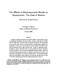
Figure 1 shows the consumption pro…les of both rational ( = 1) and hyperbolic ( = 0:7) agents. As expected, the consumption path of the rational agent is steeper than that of the hyperbolic agent’s. The reason is that faced with the same real interest rate, the more myopic hyperbolic agent opts to consume more and save less at every age than his rational counterpart. The hyperbolic agent’s consistent “undersaving” in relation to the rational agent’s results not only in a ‡atter consumption pro…le, but also in a consumption trajectory that starts turning downward immediately after retirement. In contrast, the rational agent’s post-retirement consumption path only starts declining near death. The empirical estimates for the reduction in consumption upon retirement range from 9% to 20%.14 For the retired rational agent, consumption drops abruptly by 8.51%, but for his hyperbolic counterpart, consumption falls by 10.88% right after retirement.
1 4 See, among others, Ameriks, et al. (2007), Hurd and Rohwedder (2005), Bernheim, et al. (2001) and Hamermesh (1984).
17
4.2
Raising the Retirement Age
In this section, we increase JR ; the age at which retired agents can start claiming full social security bene…ts, from 65 to 70 years old. In doing this, we implement two regimes: we either keep the social security tax rate, ss ; at the pre-reform level or hold the per capita amount of social security bene…ts, x; constant. In both cases, the new retirement policy reduces the share of social security claimants from around 18% to 12.42%. Table 2 below presents the e¤ects of these regimes on some macroeconomic aggregates. In both experiments, we observe a reduction in the post-reform real wage rate due to the increase in the supply of aggregate labor hours. Due to factor complementarity in production, the increase in the equilibrium demand for aggregate labor also increases the demand for aggregate capital, which increases the real interest rate. When ss is held constant, raising the retirement age increases the present values of expected lifetime incomes across all agent types in two ways: the extension of the working-age horizon increases the present value of lifetime labor income, and the reduction in the fraction of retired agents increases the amount of per capita bene…ts upon retirement by 42.25%. This substantial increase in expected lifetime incomes induces agents to reduce savings. Thus, aggregate savings decline, which further increases the real interest rate and reduces the amount of accidental bequests by 15.11%. In equilibrium, aggregate capital declines. The resultant decline in aggregate capital is su¢ cient to reduce aggregate output by 2.70%, which in turn, leads to a reduction of aggregate consumption by 2.02%. When the amount of per capita social security bene…ts, x; is held constant, aggregate capital still declines but by a smaller percentage than that under constant ss : The reason is that although expected lifetime labor incomes increase, there is no corresponding increase in x, which dissuades agents from reducing savings as much as in the case with constant ss so that aggregate capital also does not fall as much: This consequently prevents the equilibrium real interest rate from rising as much as in the constant- ss regime. Furthermore, as raising the retirement age reduces the number of retirees that share in the pool of pension bene…ts, keeping the amount of per capita social security bene…ts constant allows for a lower social security tax rate, ss ; which can be essentially interpreted as partial privatization of social security. Thus, raising the retirement age while keeping the level of social security bene…ts constant essentially constitutes a mixture of two policy reforms. The reduction in ss increases the after-tax real wage rate, which encourages agents to work more so that the equilibrium aggregate labor hours increase by more than that in the previous experiment. In this case, the per capita amount of unintended bequests increases with the increase in the real interest rate, in spite of the reduction in aggregate capital. Aggregate output increases by 3.39%, which in turn, raises aggregate consumption by 3.51%.
18
Table 2 Macroeconomic E¤ects of Raising the Retirement Age (in %) Experiment Constant
ss
Constant x
r
w
ss
15:61
7:84
0
7:47
3:97
x
b
42:25
33:30
0
K
L
15:11
15:84
5:58
2:21
3:80
7:67
Y
C
2:70
2:02
3:39
3:51
Tables 3 shows the welfare e¤ects of raising the retirement age from 65 to 70 years old for the two experiments. With the increase in the real interest rate, consumption pro…les across agent types become steeper after the reform as the after-tax real interest rate increases, which raises i i j+1 . Although, j+1 (i.e., the relationship between the steepness of the earnings pro…le and the growth factor of consumption in the absence of labor-leisure choice) declines, which tends to reduce future consumption, its negative impact is but miniscule.
Table 3 Welfare E¤ects of Raising the Retirement Age (in %) Constant age age age age age age
20-24 25-34 35-44 45-54 55-64 65-85
Constant x
ss
= :7 3:11 1:44 0:81 3:07 5:35 8:70
=1 3:13 1:24 1:30 3:86 6:45 10:22
2:63
age age age age age age
20-24 25-34 35-44 45-54 55-64 65-85
= :7 2:71 3:55 4:67 5:78 6:89 8:50
= :1 2:70 3:65 4:91 6:17 7:42 9:22
5:54
In both experiments, it is the groups of retired agents that gain the most advantage in raising the mandatory retirement age even when retirement bene…ts are held constant, as the extra years of work allows agents to accumulate more pre-retirement assets, which enables them to consume more during retirement. Moreover, raising the retirement age reduces the number of retirees who would split the pension bene…ts so that when ss is held constant, the amount of social security bene…ts per retiree, x; increases. We thus observe that greater gains accrue to the retired agents under a constant ss : However, the young and middle-aged workers (aged 20 to 54 years old) experience 19
higher welfare gains under a constant-x regime, as they are the ones that bene…t more in terms of lower present values of lifetime taxes owed from the reduction of the social security tax rate. Indeed, the younger cohorts (aged 20 to 34 years old) even lose from the policy reform under a constant ss mainly because they face the greatest increases in the present values of their lifetime taxes (due to the extension of their working-age horizon) and the highest declines in the present values of lifetime unintended bequests. Accordingly, the overall economy gains more under a policy reform that holds the amount of pension bene…ts, x; constant. Except for the youngest workers (aged 20-24 years old), the less myopic agents bene…t more or lose less from the reform, as they are the ones whose savings respond more to a higher equilibrium real interest rate and thus have steeper consumption pro…les. The youngest hyperbolic workers garner greater welfare gains (or incur less welfare losses) as myopia induces them into borrowing, so that the lower post-reform equilibrium real interest rate reduces their interest payments on debt.
4.3
Privatizing Social Security
Table 4 summarizes the macroeconomic e¤ects of social security privatization. We observe a considerable increase in aggregate savings of 54.05%, as privatization induces agents of all types to augment private savings in lieu of the reduction in the “forced savings” mandated by the social security system. This increase in aggregate savings, in turn, increases the amount of unintended bequests in the economy by 58.70%. In equilibrium, the increase in the supply of capital due to the increase in aggregate savings reduces the real interest rate by 21.13%. The consequent increase in the equilibrium demand for capital is matched by an increase in the demand of labor, since capital and labor are complements in production. Although the reduction in the after-tax real wage rate induces an increase in aggregate labor supply, the outward shift in the demand for labor dominates so that the equilibrium real wage rate increases by 14.29%. Together, the increases in the aggregate levels of capital and labor increase output (by 21:50%) and thus, aggregate consumption (by 19.08%).
Table 4 Macroeconomic E¤ects of Social Security Privatization (in %) r
w
b
K
L
Y
C
-21.13
14.29
58.70
54.05
6.31
21.50
19.08
Although the reduction in the post-reform real interest rate causes ‡atter consumption pro…les, all agents still gain from privatization. This happens due to the upward shifting of consumption 20
pro…les across agent types (indexed by ); as post-reform incomes rise due to the increase in labor incomes and the per capita amount of unintended bequests. As ‡atter consumption pro…les mean higher consumption levels when young and lower consumption levels when old, privatization in this case implies greater welfare gains for younger workers than that for older workers and retired agents. Indeed, Table 5 shows that the youngest workers favor the pension system the least, while the retired agents favor it the most. As in Fehr et al. (2008), the youngest workers gain the most from having the highest reduction of the present value of their lifetime taxes from the elimination of the social security tax rate and from experiencing the greatest increase in the present value of lifetime unintended bequests, which together allow them to increase their lifetime consumption the most. The retirees are disadvantaged by privatization the most, as this eliminates retirement bene…ts. This causes an abrupt reduction in post-retirement income, which severely constrains consumption. The surviving retirees lose further from privatization, as the social security system provides, what Imrohoroglu et al. (2003) refer to as an “actuarial reward for survival.”This ranking of welfare gains is consistent with Imrohoroglu et al. (2003) although in their setup even the retired rational agents gain from privatization mainly due to the presence of liquidity constraints that are relaxed upon the elimination of social security.15 On an aggregate level, welfare gains accrue to the entire economy. Except for the youngest workers, the more present-biased workers gain more from the privatization of social security. The youngest, more myopic workers gain less than their less myopic counterparts because greater myopia induces them to incur greater current debt, which leaves them less resources for next-period consumption. For the rest of the older, more myopic workers, the increase in disposable incomes due to the elimination of the social security tax, encourages them to increase consumption more than their less myopic counterparts so that they are able to experience higher welfare gains. Moreover, under a no social security regime, the rest of the more myopic agents know that the abrupt decline in their retirement consumption due to myopia would be aggravated by the absence of the commitment mechanism that the “forced savings”under social security a¤orded them. Since it is the hyperbolic agents that value post-retirement consumption more (or discount post-retirement consumption less than their rational counterparts), they are the ones that increase their asset holdings more all throughout their middle-age and latter working days. Consequently, consumption levels for the more myopic retirees do not fall as much. 1 5 Indeed for the same reason, Fehr et al. (2008) …nd that relaxing borrowing constraints reduces the long-run welfare gains from privatization.
21
Table 5 Welfare E¤ects of Social Security Privatization (in %)
age age age age age age
20 25 35 45 55 65
24 34 44 54 64 85
= :7
=1
18:28 15:66 12:26 8:99 5:85 1:50
18:32 15:36 11:54 7:90 4:41 0:35
9:89
We thus observe that younger cohorts bene…t considerably more while retirees bene…t considerably less under social security privatization than under either one of the aforementioned regimes that postpones retirement. The younger workers gain signi…cantly from the relaxation of their liquidity constraints upon the abolition of social security taxes, while retirees either lose or gain to a lesser extent due to the complete elimination of their pension bene…ts. It thus appears that if the institution of these reforms were put to a vote, the younger workers would vote for privatization while the older workers and retirees would vote for postponing retirement. The voting outcome would depend on the welfare weights used in aggregating welfare. In this instance, using a simple weighted average places privatization at a greater advantage.
4.4
Changing the Fraction of QHD Agents
In order to ascertain the externalities imposed by the existence of time-inconsistent discounters on the rest of the economy, we systematically change the fraction of hyperbolic agents while still allowing the policy reforms to take place. We denote the fraction of hyperbolic agents in the economy by 1 2 (0; 1): 4.4.1
Raising the Retirement Age
Figure 2 below shows that the in both experiments, increasing the fraction of hyperbolic agents, 1 ; increases the equilibrium real interest rate up to a critical value and decreases it above this value: This happens because as the economy becomes more populated with myopic hyperbolic agents, undersaving is aggravated, which causes the equilibrium real interest rate, r; to rise. However, further increasing 1 ; which raises r even further, allows agents to work less via the income e¤ect.
22
This leads to a reduction in the equilibrium level of aggregate labor hours. The reduction in the demand for labor reduces the demand for aggregate capital, which consequently, tends to reduce the equilibrium real interest rate for higher values of 1 . This is key to explaining the welfare patterns that are presented below.
In Table 6, we observe the welfare e¤ects of raising the retirement age as we increase 1 under a constant- ss regime: When 1 is low enough, the younger hyperbolic workers lose less than their rational cohorts after the reform. This is because increasing 1 (when it is low enough) which raises r; increases the interest debt of the younger hyperbolic workers so that they could not a¤ord to reduce their savings as much as their rational counterparts in response to the mandatory increase in the retirement age. This allows the former group to support a greater increase in equilibrium consumption, and thus, higher welfare gains. However, as 1 increases further, the real interest rate starts decreasing, which lowers the interest debt payments of the young hyperbolic workers so that greater myopia now induces them to reduce savings more than their rational counterparts. Accordingly, the former group’s post-reform welfare losses become higher than that of the latter. For the older sector of the workforce (who are now all savers), the less present-biased agents consistently gain more than their more myopic counterparts, as it is the former group that experience higher post-reform consumption levels from having steeper consumption pro…les. For the younger rational workers (aged 20 to 34 years old) and most of the hyperbolic workers (aged 20 to 54 years old), the welfare pattern that we observe is as follows: the welfare gains (losses) decrease (increase) up to an age-speci…c critical value, b1;j ; and increase (decrease) above 23
this critical value: The reason is that when r increases as 1 rises, agents are induced to save less as the income e¤ect dominates after the retirement age is extended. This then reduces equilibrium consumption, and thus welfare. However, when r starts falling the further 1 is increased, agents are now induced to save more (still via the income e¤ect), which allows a greater amount of consumption to be supported in equilibrium. Thus, welfare increases. For the older workers and retirees, welfare levels monotonically increase with 1 even when 1 < b1;j : This is because when r increases as 1 (< b1;j ) increases, these sectors of the workforce are the ones that are a¤ected the most from the consequent reduction in the present value of their lifetime bene…ts. Thus, the higher r prompts them to save more, which allows them to consume more and experience higher welfare gains as b1;j ) rises, the present 1 rises. In the same line of reasoning, when r starts falling as 1 (> value of their liftime bene…ts rise considerably so that they are able to gain increasingly more after the reform. The overall welfare gains follow a U-shaped pattern as the economy becomes more populated by hyperbolic agents. This merely re‡ects the pattern that we observe for a majority of the age groups.
Table 6 Welfare E¤ects of Raising the Retirement Age (in %; constant 1
age age age age age age
20 25 35 45 55 65
24 34 44 54 64 85
=0 =1
= 0:1 = :7 =1
= 0:5 = :7 =1
3:20 1:40 1:01 3:42 5:83 9:32
3:03 1:41 0:78 2:97 5:17 8:37
3:11 1:44 0:81 3:07 5:35 8:70
2:55
1
3:32 1:48 0:99 3:46 5:94 9:53
2:54
1
2:63
3:12 1:24 1:30 3:86 6:45 10:22
ss )
= 0:9 = :7 =1 1
2:21 0:68 1:40 3:52 5:69 8:94 2:92
1:94 0:20 2:16 4:57 7:04 10:70
=1 = :7
1
1:78 0:32 1:68 3:73 5:84 9:01 3:07
Table 7 presents the results under a constant x. We generally observe the same U-shaped pattern of welfare gains (as 1 increases) for rational agents aged 20 to 44 years old and for hyperbolic aged 20 to 54 years old. Also, just like in the previous experiment, the older rational workers experience monotonic increases in welfare as 1 is increased. However, for the older and retired hyperbolic workers, welfare starts decreasing as 1 is further increased above a certain threshhold. This happens because unlike in the previous experiment where the corresponding reduction in r is met by a substantial increase in the present value of lifetime bene…ts, which enables retirees to increase equilibrium consumption and thus welfare, the hyperbolic retiree’s welfare gains, in this case, start
24
decreasing as r goes down due to two reasons: 1) the increase in the present value of lifetime pension claims is not as high under a constant-x regime than under a constant- ss regime; and 2) myopia induces a reduction in savings in the face of an increase in the present value of lifetime bene…ts. Accordingly, the older and retired hyperbolic agents experience falling consumption levels and thus, welfare gains, as 1 approaches unity. In the aggregate, the welfare level from raising the retirement age increases as the economy becomes more populated with hyperbolic agents.
Table 7 Welfare E¤ects of Raising the Retirement Age (in %; constant x) 1
Age 20 25 35 45 55 65
24 34 44 54 64 85
=0 =1
= 0:10 = :7 =1
= 0:50 = :7 =1
2:93 3:72 4:77 5:81 6:83 8:29
3:18 3:94 4:95 5:95 6:94 8:37
2:71 3:55 4:67 5:78 6:89 8:50
5:42
1
1
2:73 3:58 4:72 5:84 6:95 8:54
5:44
5:54
2:70 3:65 4:91 6:17 7:42 9:22
= 0:90 = :7 =1 1
3:24 3:95 4:90 5:86 6:83 8:27 5:60
3:69 4:49 5:57 6:67 7:66 9:38
=1 = :7
1
3:52 4:16 5:03 5:91 6:81 8:14 5:62
In both cases, we observe that the highest aggregate welfare gains accrue to the economy with purely hyperbolic agents. This is because it is the more myopic, hyperbolic agents that bene…t more in terms of greater increases in lifetime labor incomes from having the retirement age raised mandatorily. For time-inconsistent agents, the external imposition of an extended working-period horizon functions like another pre-commitment device that constrains them to increase lifetime savings. 4.4.2
Privatizing Social Security
In Figure 3 below, we observe that as the fraction of hyperbolic agents is increased up to some critical value, e1 ; the real interest rate increases. However, further increasing 1 above e1 ; reduces the real interest rate. As in the preceding simulated reform, this can be explained as follows: as the economy becomes inhabited by more myopic hyperbolic agents, aggregate undersaving becomes more severe, which pushes up the real interest rate, r: When r increases, both substitution and income e¤ects come to play. While the substitution e¤ect occasions an increase in savings due to the reduction in the relative price of future consumption, the income e¤ect motivates a reduction in savings due to the increase in interest income. When r further rises as 1 continues to increase, 25
the substitution e¤ect starts dominating, as there are now more hyperbolic agents, who have to save more in response to privatization. This now tends to reduce r: Moreover, increasing r further induces agents to reduce their labor hours so that the equilibrium level of aggregate labor hours decreases. The consequent decline in the equilibrium aggregate demand for labor reduces the aggregate demand for capital due to labor-capital complementarity in the production function. This also tends to reduce the equilibrium real interest rate as more and more hyperbolic agents start dominating the population.
Table 8 below shows that as the hyperbolic agents start crowding the economy (i.e., when 1 > :5), rational agents start gaining more from privatization than the hyperbolic agents. This happens because the real interest rate falls su¢ ciently enough to dissuade the more myopic hyperbolic agent from increasing savings as much as that of his rational neighbor. This then allows the latter to experience a higher consumption level in equilibrium. For rational agents, increasing 1 increases their welfare gains up to a critical level, eij ; but reduces these gains above it: The reason is that when r increases as 1 initially rises, these agents save more and are able to support a greater level of consumption in equilibrium. However, further increasing 1 ; which starts reducing the real interest rate, induces these agents to reduce savings, which reduces equilibrium consumption and thus, welfare. In this light, we remark that a su¢ ciently small number of hyperbolic agents generates positive pecuniary externalities on their rational counterparts, while one too many of these agents in the population imposes negative pecuniary externalities on rational agents. For hyperbolic agents, welfare decreases successively as myopia becomes more endemic in the economy. The overall welfare gain, ; decreases with 1 below a critical value, while it increases with 1 26
above this critical level. This pattern re‡ects the rise and fall of the equilibrium real interest rate as 1 is increased (after its initial decline due to privatization). For our given set of parameters, a mixed population composed of half rational and half myopic agents generates the greatest overall welfare gains from privatization. It thus appears that social security privatization becomes even more attractive in an economy composed of both rational and hyperbolic agents.
Table 8 Welfare E¤ects of Privatizing Social Security while Increasing 1
age age age age age age
20 25 35 45 55 65
24 34 44 54 64 85
=0 =1
18:25 15:19 11:25 7:53 3:99 0:80 9:14
1 = 0:10 = :7 =1
19:32 16:59 13:07 9:72 6:51 2:11
18:31 15:26 11:35 7:64 4:11 0:66
9:43
= :7
= 0:5 =1
18:28 15:66 12:26 8:99 5:85 1:50
18:78 15:36 11:84 8:14 4:60 0:18
1
9:89
1
(in %)
1 = 0:90 = :7 =1
16:47 14:03 10:84 7:73 4:68 0:36 9:50
17:51 14:73 11:11 7:60 4:18 0:58
=1 = :7
1
15:74 13:39 10:29 7:25 4:24 0:04 8:40
We further note that in this particular parameterization, the retired hyperbolic agents in a mixed-population economy gain from privatization while retired hyperbolic agents loses in an economy purely populated by hyperbolic agents (i.e., when 1 = 1). This is in line with our earlier observation that the higher r due to the pecuniary externalities generated by hyperbolic agents in a mixed economy allows these agents to save more in response to privatization. The higher post-reform savings by hyperbolic agents then allows them to support higher post-reform levels of retirement consumption.
5
Concluding Comments
This paper mainly contributes to the existing literature on the long-run viability of the social security system by evaluating the macroeconomic and welfare consequences of raising the retirement age in the U.S and comparing these e¤ects to those from privatizing the public pension system. We do this using a 65-period, general equilibrium, overlapping generations economy inhabited by both rational and quasi-hyperbolic agents, who face mortality risks. The co-existence of both rational and quasi-hyperbolic discounters allows us to ascertain the aggregate and welfare externalities generated by the latter agent type. By abstracting from borrowing constraints and income uncertainty, we 27
derive an analytical solution to the system using the solution concept of …rst-order Markov perfect equilibria. In raising the retirement age from 65 to 70 years old, we consider two alternative regimes: we either hold constant the social security tax rate or keep the amount of per capita social security bene…ts constant. In both cases, aggregate capital decreases, as the increases in the expected lifetime labor incomes induce agents to reduce savings, while aggregate labor increases from the compulsory extension of the working-age horizon. Accordingly, the reform’s impacts on aggregate output and aggregate consumption are ambiguous, in contrast to the expectation that raising the retirement age would raise the standard of living. Our numerical results show that under a constant-bene…ts regime, aggregate output and consumption increase, while these decrease under a constant-tax rate regime. On an aggregate level, this policy reform is welfare-increasing. However, under a constant-social security tax rate regime, the youngest workers incur welfare losses from the reform primarily due to the increase in their expected discounted lifetime tax liabilities and a considerable reduction in the amount of unintended bequests. Under a constant-bene…ts regime, agents of all ages and discounting types gain, as the subsequent reduction in the social security tax rate signi…cantly relaxes their liquidity constraints. The quantitative results thus imply that postponing retirement under the latter regime is preferable to the former regime, unless some compensation scheme is instituted for the younger cohorts. The presence of hyperbolic agents in the economy indeed imposes a pecuniary externality on the rest of the economy. In particular, we observe that the real interest rate exhibits an inverted U-shaped pattern as the fraction of hyperbolic agents is increased. As the percentage of hyperbolic agents increases, aggregate undersaving worsens, which causes the real interest rate to rise. A rising real interest rate, however, depresses the real wage rate, which induces agents to work less so that equilibrium labor hours go down. Labor-capital complementarity in production reduces the demand for aggregate capital subsequent to the decrease in the demand for aggregate labor. This tends to reduce the equilibrium real interest rate as hyperbolic agents begin to crowd the economy. We revisit the issue of social security privatization in our model economy. Interestingly, we …nd that the aggregate welfare gain follows the trajectory of the real interest rate as the fraction of hyperbolic agents is increased. We thus observe that social security privatization is most desirable with a mixed population of rational and hyperbolic agents. Moreover, we …nd that retired hyperbolic agents gain after privatization in a mixed economy, while they lose in a economy purely composed of time-inconsistent individuals. These observations imply that ignoring the externalities generated by hyperbolic agents may lead to spurious welfare conclusions. In the context of raising the retirement age, the highest aggregate welfare gains accrue to the economy with a greater population of hyperbolic agents. This suggests that the mandatory postponement of retirement serves as another pre-commitment device for time-inconsistent agents
28
to increase their lifetime savings. Comparing the welfare e¤ects of social security privatization to those of raising the retirement age, we …nd that the younger workers would prefer the former, while older workers and retirees would opt for the latter reform. That the aggregate welfare gain under privatization is greater than that under delayed retirement might be primarily because we have not considered the costs of transitioning to a fully privatized pension system in order to reference the long-run analyses of Imrohoroglu et al. (2003). Moreover, we have abstracted from incorporating into the model the reported physiological and psychological bene…ts (see Butrica et al., 2006) that older agents gain from continuing to work during the “golden age years.”Taking account of these considerations may serve to strengthen the arguments in favor of raising the legal retirement age and can thus be a subject for future research.
References [1] Ainslie, G. (1992). Piconomics. Cambridge, NY: Cambridge University Press. [2] Ameriks, J., Caplin, A., & Leahy, J. (2007). Retirement consumption: Insights from a survey. The Review of Economics and Statistics 89(2), 265-274. [3] Angeletos, G., Laibson, D., Repetto, A., Tobacman, J., & Weinberg, S. (2001). The hyperbolic consumption model: calibration, simulation, and empirical evaluation. Journal of Economic Perspectives 15, 47-68. [4] Arias, E. (2010). United States life tables, 2006. National Vital Statistics Reports 58(21), 1-40. [5] Bernheim, D., Skinner, J. & Weinberg, S. (2001). What accounts for the variation in retirement wealth among U.S. households. American Economic Review 91, 1-26. [6] Bernstein, A. (2005, January 24). Social security: Are private accounts a good idea? BusinessWeek. Retrieved from http://www.businessweek.com. [7] Butrica, B., Schaner, S., & Zedlewski, S. (2006, May 23). Enjoying the golden work years. Urban Institute Research of Record. Retrieved from http://www.urban.org/UploadedPDF/311324_golden_work_years.pdf. [8] Calvo, E. (2006). Does working longer make people healthier and happier Work Opportunities for Older Americans Brief, Series 2. Chestnut Hill, MA: Center for Retirement Research, Boston College. [9] Cendrowicz, L. (2010, July 8). Will Europe raise the retirement age? TIME Business. Retrieved from http://www.time.com. 29
[10] Diamond, P. (1965). National debt in a neoclassical growth model. American Economic Review 55, 1126-1150. [11] Diamond, P. & Koszegi, B. (2003). Quasi-hyperbolic discounting and retirement. Journal of Public Economics 87, 1839-1872. [12] Diaz-Jimenez, J., & Diaz-Saavedra, J. (2009). Delaying retirement in Spain. Review of Economic Dynamics 12, 147-167. [13] Fehr, H., Habermann, C., & Kindermann, F. (2008). Social security with rational and hyperbolic consumers. Review of Economic Dynamics 11, 884-903. [14] Frederick, S., Loewenstein, G., & O’Donoghue, T. (2002). Time discounting and time preference: a critical review. Journal of Economic Literature 40, 351-401. [15] Friedman, B., & Warshawsky, M. (1990). The cost of annuities: Implications for saving behavior and bequests. Quarterly Journal of Economics 105, 135-154. [16] Hamermesh, D. (1984). Consumption during retirement: The missing link in the life cycle. Review of Economics and Statistics 66, 1-7. [17] Hurd, M. & Rohwedder, S. (2005). The retirement-consumption puzzle: Anticipated and actual declines in spending at retirement. RAND Labor and Population Working Paper Series, WR242. [18] Imrohoroglu, A., Imorohoroglu, S., & Joines, D.H. (1995). A life-cycle analysis of social security. Economic Theory 6, 83-144. [19] Imrohoroglu, A., Imorohoroglu, S., & Joines, D.H. (1999). Social security in an overlapping generations economy with land. Review of Economic Dynamics 2, 638-665. [20] Imrohoroglu, A., Imorohoroglu, S., & Joines, D.H. (2003). Time-inconsistent preferences and social security. Quarterly Journal of Economics 118, 745-784. [21] Kotliko¤, L. (1996). Privatization of social security: how it works and why it matters? In J. Poterba (Ed.), Tax Policy and the Economy (pp. 1-32). MIT Press: Cambridge. [22] Kotliko¤, L. (1998). Simulating the privatization of social security in general equilibrium. Quarterly Journal of Economics 118, 745-784. [23] Krusell, P., & Smith, A. Jr. (2003). Consumption-savings decisions with quasi-geometric discounting. Econometrica 71, 365-375.
30
[24] Kumru, C., & Thanapoulos, A. (2008). Social security and self-control preferences. Journal of Economic Dynamics and Control 32, 757–778. [25] Laibson, D. (1997). Golden eggs and hyperbolic discounting. Quarterly Journal of Economics 112, 443-447. [26] Laibson, D. (1998) Life-cycle consumption and hyperbolic discount functions. European Economic Review 42, 861-871. [27] Macurdy, T. (1981). An empircal model of labor supply in a life-cycle setting. Journal of Political Economy 89, 1059-1085. [28] McDaniel, C. (2007). Average tax rates on consumption, investment, labor and capital in the OECD 1950-2003. Mimeo, Arizona State University. [29] Mehra, R., & Prescott E.C. (1985). The equity premium: A puzzle. Journal of Monetary Economics 15(2), 145-161. [30] Mermin, G., & Steuerle, E. (2006). Would raising the social security retirement age harm low-income groups. Retirement Policy Project Series Brief 19. Retrieved from http://www.urban.org/UploadedPDF/311413_Raising_Retirement_Age.pdf. [31] Nishiyama, S. & Smetters, K. (2007). Does social security privatization produce e¢ ciency gains? Quarterly Journal of Economics 122, 1677-1719. [32] Okello, C., & Charlton, A. (2010, June 28). French teens protest against raising the retirement age. The Times Leader. http://www.timesleader.com. [33] Peleg, B., & Yaari, M. (1973). On the existence of a consistent course of action when tastes are changing. Review of Economic Studies 40, 391-401. [34] Phelps, E., & Pollack, R. (1968) On second-best national saving and game-equilibrium growth. Review of Economic Studies 35, 185-199. [35] Rainsford, S. (2011, January 28) Spain strikes deal over raising of retirement age. BBC Madrid. Retrieved from http://www.bbc.co.uk/news/business-12305246. [36] Soman, D., Ainslie, G., Frederick, S., Li, X., Lynch, J., Moreau, P., Mitchell, A., Read, D., Sawyer, A., Trope, Y., Wertenbroch K., & Zauberman G. (2005) The psychology of intertemporal discounting: why are distant events valued di¤erently from proximal ones? Marketing Letters 16, 347–360. [37] Strotz, R. (1956) Myopia and inconsistency in dynamic utility maximization. Review of Economic Studies 23, 165-180. 31
[38] Weller, C. (2001, October 1). Raising the retirement age: The wrong direction for social security. Economic Policy Institute Brie…ng Paper. Retrieved from http://www.epi.org/publication/brie…ngpapers_raisingretirement_raisingretirement/.
32
Appendix Proof of Proposition 1. This proposition is proven by backward induction. Consider the retirement period j = JR ; ..., J 2; J 1 and J: Since hij = 0 for all i; it follows that ij = 0 throughout the retirement period. Also, u(cij ; hij ) = u(cij ; 0) for all i and j: At the terminal age J, optimal consumption is given by cij = (1 + re)aij 1 + (qyJ + yJ 1 ) and labor hours is zero. Hence iJ = 1: Consider age J 1: The agent’s problem is now given by
ciJ ;ciJ
u(ciJ
maxi
i 1 ;hJ ;hJ
1 ; 0)
+
i J u(cJ ; 0)
i
1
subject to the consolidated budget constraint ciJ
1
(1 + re)aiJ
+ qciJ =
1 + (qyJ + yJ 1+ c
1)
:
(26)
From the Euler equation for consumption, we get ciJ = [
J (1
i
Hence, i J
where
Hence,
i J
i J
= 1 and
i J 1
=1+
Consider age J
e)] J (1 + r
[
i J
q
1
i J
and
=
1
1
i i J i J
1
i i J cJ 1
= 1: Substituting ciJ = ciJ
1
+ re)] ciJ
;
into (6) gives
(1 + re)aiJ 1 + (qyJ + yJ 1 ) : (1 + c ) 1 + iJ q iJ i J 1
= 0::
2. The agent’s problem is now given by u(ciJ
max
fcij ;hij gJ j=J
2 ; 0)
+
i
J 1
u(ciJ
1 ; 0)
+
i J u(cJ ; 0)
2
subject to (1 +
i c )cJ 2
+ aiJ
1
= (1 + re)aiJ 33
2
+ yJ
2;
(27)
ciJ and ciJ =
i i J cJ 1 :
=
1
Using ciJ = u(ciJ
i i J cJ 1 ;
2 ; 0)
1 c)
(1 +
+
=)
2 ; 0)
ciJ
=)
=
i
i
J 1
ciJ 1
h
1+
=
ciJ
2
=) ciJ Hence,
i J 2
At j = JR
=1+
=
i J 1
+ re) h
1+
=
+ re) h
1+ {z
1 ; 0):
i
i 1 J
i
i 1 J
J
ciJ
1 1
1
1
ciJ
2:
}
1
i i J 1 i J 1
1
dciJ daiJ
1 ; 0)
1
+ re)
(1 + re)aiJ i J 1
c) 1 +
i J 1
u0c (ciJ
J
2
1
q
i
i 1 J
u(ciJ
;
Combining (7) and (8) gives
i i J 1 cJ 2
(1 +
(28)
i J 2
and
q
i J 1
= 0:
+ yJ 2 + q(qyJ + yJ 1+ c (1 + re)aiJ
2
+
J 2
1)
:
1; the consumer’s objective function is
max J
fcik ;hik g
k=JR
subject to
2
is
J
J 1 (1
i J:
i J 1
+q
=
i 1 J
J
;
J 1
i
i 1 J
J
i J
i J 1
1+
1
1+
J 1 (1 i J 1
|
i J 1
h
J 1 (1 i J 1
i
i
Hence,
where
J 1
=
2
+
1
we can rewrite the objective function as
The …rst-order condition with respect to aiJ u0c (ciJ
(1 + re)aiJ
i J 1
1
8 < u(ci : JR
i 1 ; hJR 1 )
(1 +
+
i
2 4
J X
m j 1
m=j+1
i c )cJR 1
+ aiJR = (1 + re)aiJR 34
0 @
m Y
d
d=j+1
1
+ y JR
1;
1
A u cim ; him
39 = 5 : ;
ciJR
1
=
i JR
"
and cij+1 =
(1 + re)aiJR + 1+ c
i i j+1 cj
i JR
#
;
for j = JR ; :::; J:
From the …rst-order condition for labor hours, we have: uc ciJR
i 1 ; h JR 1
w" e JR
1
= uh ciJR
Given the speci…c form of the utility function, hiJR
ciJR
c)
=)
ciJR 1
1
=
=)
Hence,
i JR 1
=1+
i JR
+q
i i JR cJR 1
"
1 i JR
1+ ciJR 1
i JR
q
=
i JR
q 1
i JR 1
i JR :,
"
i JR
+
= (1 + re)aiJR
(1 + re)aiJR 1 + 1+ c
(1 + re)aiJR 1 + 1+ c
i JR 1
q
1 k j k=JR 1 q
Suppose the desired results hold for ages j + 1; j + 2; :::; J i i j+m+1 cj+m
cj+m+1 = for m = 1; :::; J
j
q
JR 1
for all i:
+ yJR
1
JR 1
PJR
:
1= 1 =A)
= (w" e JR
1
From the …rst-order condition for aiJR : (1 +
i 1 ; h JR 1
i JR
i JR 1
i k+1
1
+q
i JR
#
;
#
i k+1
.
1 and J: This means
i j+m+1 ;
+
JR
(29)
1; and cij+1 =
1 i j+1
(1 + re)aij+1 +
i j+1
j+1
We want to show that (16) holds for m = 0 and cij = (1 + re)aij + problem at age j is given by max J fcik ;hik gk=j
8 < u(ci ; hi ) + : j j
i
2 4
J X
m j 1
m=j+1
35
0 @
m Y
d=j+1
:
j
(30)
i j
=
i j:
The consumer’s
39 = A u(cim ; him )5 d ; 1
subject to (16), (17) and cij + aij+1 = (1 + re)aij + yj:
(31)
Using (16), we can rewrite the objective function as follows:
u(cij ; hij ) +
i
2 4
J X
m j 1
m=j+1
= u(cij ; hij ) +
= u(cij ; hij ) +
= u(cij ; hij ) +
i
i
i
2 4
0 @
j+1
j+1
d
d=j+1
i i j+1 u(cj+1 ; hj+1 )
2
m Y
+
1
3
A u(cim ; him )5 i i j+2 u(cj+2 ; hj+2 )
j+1
0
2
41 +
j+2
(
@
J Y
m
m=j+1
1 j+2 )
1
1
3
A u(ciJ ; hiJ )5
3 i i u(c ; h ) J j 1@ J J A 5 u(cij+1 ; hij+1 ) m i i u(c ; h ) j+1 j+1 m=j+2 13 J h i Y 1 A5 u(cij+1 ; hij+1 ): + ::: + @ m ( m)
u(cij+2 ; hij+2 ) + ::: + j+2 u(cij+1 ; hij+1 ) 0
41 +
J j 1
+ ::: +
0
J Y
m=j+2
The agent’s problem can now be rewritten as 8 < max u(cij ; hij ) + aj+1 :
i
j+1
2
41 +
j+2
(
0
1 j+2 )
+ ::: + @
J h Y
m
(
1 m)
m=j+2
subject to (17) and (18)
i
9 = A5 u(cij+1 ; hij+1 ) ; 13
The …rst-order condition with respect to aij+1 is
1+
cij
(hj ) A 1+
!
=
i
e) j+1 (1 + r i j+1
2
41 +
j+2
(hj+1 ) A 1+
1 j+2 )
+ ::: + @
J h Y
m=j+2
1+
cij+1
(
0
!
Hence,
36
:
m
(
1 m)
i
13 A5
cij+1
i
= |
8 J l < h X Y (1 + r e ) j+1 1 + i : j+1 l=j+2 m=j+2 {z
(
m
91 i=
1
m)
;
i j+1
cij
"
+ A
}
1+
i j+1
(hj+1 )
1+
This establishes equation (8). Combining (17) and (18) gives 8 > > < i (1 + c )cj + (1 + c ) q > > : | =)
Hence,
i j
=1+q
cij
i j+1
=
i j
i j+1
|
{z
{z
aij+1
i j+1
i j
+
cij+1
1
1+q
and
i j+1 cj
=q
j+1
i j
q
}
"
+q
(1 + re)aij + 1+ c
JR 1 k j k=j q
37
j+1
i k+1
j+1
j
i k+1 :
9 > > = > > ; } i j
= (1 + re)aij + yj #
:
Q.E.D.
1+
(hj )
#
: