On the geometry of a generalized cross-correlation random field F. Carbonell∗ and K. J. Worsley Department of Mathematics and Statistics, McGill University, Montreal, Canada
Abstract Studying the geometry of random fields (RF) has become a well established tool for dealing with the statistical problem of multiple comparisons. This has leaded to an increasing number of applications in medical imaging and astrophysics mainly. In particular, cross-correlation RF, defined as the sample correlation between pairs of independent Gaussian RF, have been used for analyzing functional connectivity in brain images. However, in some cases one needs to deal with correlated observations for which the "independece " assumption is not longer valid. In this paper we define a generalized cross-correlation RF that allows for correlated observations. We also study the geometry of such RF by giving results for the expected Euler Characteristic of its local maxima.
1
Introduction
During the last years Random Field Theory has became an important tool in different areas of applied probability. This is due to the many applications that have emerged principally in medical imaging and astrophysics Gott III et al. (1990), Beaky et al. (1992), Vogeley et al. (1994), Worsley (1995a), Worsley (1995b), Cao and Worsley (2001), Worsley (2003), Taylor and Worsley (2008). In particular, cross-correlation random fields have been defined for analyzing functional connectivity in brain images, where the main idea is to establish a connectivity between two different regions of the brain on the basis of a similar functional response. A general approach has been estimating connectivity within images or between pairs of images by the sample correlation between all pairs of voxels Worsley et al. (1998), Cao and Worsley (1999), Worsley et al. (2005). Thus, the challenging statistical problem is how to assess the P-value of local maxima of the resulting cross-correlation random field. Let X(s) =(X1 (s), ...., Xν (s)), s ∈ S ⊂ RM and Y(t) =(Y1 (t),...., Yν (t)), t ∈ T ⊂ RN be vectors of ν independent identically distributed smooth stationary Gaussian RF with mean 0. Then the M + N -dimensional cross-correlation RF C(s, t) is defined by the sample correlation Cao and Worsley (1999) X(s)0 Y(t) C(s, t) = q . X(s)0 X(s)Y(t)0 Y(t)
An alternative way of defining C(s, t) is via linear models. Indeed, by fitting the linear model Y(t) =X(s)β(s, t) + σ(s, t) , it can be shown that
where
∼ N (0, Iν )
b t) b (s, t) σ β(s, q C(s, t) = q , b t)) Y(t)0 Y(t) V ar(β(s, b t) = (X0 (s)X(s))−1 X0 (s)Y(t), β(s,
b (s, t) = Y(t)0 (Iν − X(s)(X0 (s)X(s))−1 X0 (s))Y(t) σ
are the maximum likelihood estimators of β(s, t) and σ(s, t), respectively. ∗ This
work was supported by a postdoctoral fellowship from the ISM-CRM, Montreal, Quebec, Canada.
1
(1)
The motivation for the present work comes from practical applications. In many brain imaging studies, the Gaussian RF Y(t) models functional Magnetic Resonance Imaging (fMRI) data, which consist on a series of ν temporal correlated observations Yi (t), i = 1, ..., ν. Hence, the classical results for the P-value of local maxima of C(s, t) given in Cao and Worsley (1999) are no longer valid in such cases. The aim of this work is to extend the results of Cao and Worsley (1999) to a more general situation with non independent observations, which corresponds to the case ∼ N (0, Σ), where Σ > 0 is a global (for all t) covariance matrix. As above, the generalized cross-correlation RF shall be defined via linear models and corresponding results for the P-value of its local maxima are obtained.
2
The geometry of random fields
The key idea consists on approximating the P-value that the local maximum exceeds a high threshold value via the geometry of the excursion set, the set of points where the RF exceeds the threshold value. For high thresholds the excursion set consists of isolated regions,each containing a local maximum, where the number of such regions is determined by the Euler characteristic (EC) of the set. Then for high thresholds near the maximum of the RF, the EC takes the value one if the maximum is above the threshold, and zero otherwise. As a consequence, for high thresholds, the expected EC approximates the P-value of the maximum of the RF. Let C = C (u) , u ∈ U ⊂ RD be a real valued isotropic RF and let S be a compact subset of RD with a . twice differentiable boundary ∂S...Let’s denote the first derivative of C by C and the D × D matrix of secondorder partial derivatives of C by C. Moreover, for any vector, we shall use subscripts j and |j to denote the jth component and the first j components, respectively. Similarly, for any matrix, the subscripts |j will denote the submatrix of the first j rows and columns. For any scalar b, let b+ = b if b > 0 and zero otherwise. Then, the d-dimensional Euler Characteristic (EC) density is defined as .+
..
.
ρd (c) = E(C d det(−C |d−1 ) | C |d−1 = 0, C = c)φ|d−1 (0, c)
(2) .
where E (·) denotes mathematical expectation and φ|d−1 (·, ·) is the joint probability density function of C |d−1 and C. Let ad = 2π d/2 /Γ(d/2) be the surface area of a unit (d − 1)−sphere in RD . Define μD (S) to be the Lebesgue measure of S and μd (S), d = 0, ..., D − 1 to be the d−dimensional intrinsic volume or Minkowski functional Z 1 detrD−1−d (M)ds, μd (S) = aD−d ∂S with M denoting the inside curvature matrix of ∂S at the point s. The expected EC χ of the excursion set Ac = {u ∈ U : C(u) ≥ c} of C above the threshold c inside S is given by E(χ(Ac )) =
D X
μd (S) ρd (c)
(3)
d=0
where ρ0 (c) = P(C ≥ c). Then, the P-value of the maximum of C inside S is well approximated by µ ¶ P max C ≥ c ≈ E(χ(Ac )). s∈S
(4)
For the particular case of the cross-correlation random field C(s, t) it was shown the following result. Lemma 1 (Lemma 3.1 in Cao and Worsley (1999))Suppose that a RF C(s, t) is stationary in (s, t) and isotropic in each of the two arguments for every fixed value of the other one, and satisfies the usual regularity conditions. Let Ac be the excursion set of C defined as Ac = {s ∈ S, t ∈T : C(s, t) ≥ c}. Then E(χ(Ac )) =
M X N X
μi (S) μj (T ) ρij (c),
i=0 j=0
where ρij (c) has the same expression as in (2) with the parameters of the RF restricted to the first i components of s, and the first j components of t. 2
3
Generalized cross-correlation random field
Let Σ > 0 be a (known) fixed symmetric matrix and consider the linear model Y(t) =X(s)β(s, t) + σ(s, t) ,
∼ N (0, Σ).
(5)
The generalized cross-correlation random field is defined by X(s)0 Σ−1 Y(t) R(s, t) = q , X(s)0 Σ−1 X(s)Y(t)0 Σ−1 Y(t)
which results from the generalized least square estimator of the coefficient β(s, t). As in Cao and Worsley (1999), it is very useful to represent the first and second order partial derivatives of R(s, t) in terms of independent random variables. Assume that Λx and Λy are the common variance matrices 1
s
t
1
of the components of (Σ− 2 X) and (Σ− 2 Y), respectively (see Section 4 for numerical approximations to Λx and 1 1 1 1 Λy ). Here, Σ 2 denotes the square root of the matrix Σ (i.e. (Σ 2 )2 = Σ) and Σ− 2 = (Σ 2 )−1 . Then, one has the following lemma. Lemma 2 The first two derivatives of R(s, t) can be rewritten as s
1
1
t
1
1
1
1
R = (1 − R2 ) 2 a− 2 Λx2 zx , R = (1 − R2 ) 2 b− 2 Λy2 zy , ss
R tt
R st
R
1
1
1
1
1
= Λx2 (−Ra−1 zx z0x − Ra−1 Qx − (1 − R2 ) 2 a−1 (zx wx0 + wx z0x ) + (1 − R2 ) 2 a− 2 Hx )Λy2 , 1
1
1
1
1
= Λy2 (−Rb−1 zy z0y − Rb−1 Qy − (1 − R2 ) 2 b−1 (zy wy0 + wy z0y ) + (1 − R2 ) 2 b− 2 Hy )Λy2 , 1
1
1
1
= Λx2 (−R(ab)− 2 zx z0y + (ab)− 2 Qxy )Λy2 ,
where b ∼ χ2ν , zx , wx ∼ N ormalM (0, IM ), zy , wy ∼ N ormalN (0, IN ), Hx ∼ N ormalM×M (0, V (IM )), Hy ∼ N ormalN ×N (0, V (IN )), ∙ ¸ Qx Qxy Q = ∼ W ishartM+N (IM+N , ν − 2), Qyx Qy a = X0 Σ−1 X distributes as a Gaussian quadratic form, all independently and independent of R. Proof. It easily follows from applying Lemma 4.2 in Cao and Worsley (1999) to the RF e e 0 Y(t) X(s) R(s, t) = q , e 0 X(s) e Y(t) e 0 Y(t) e X(s)
1
1
− − e e = Σ 2 Y(t). where X(s) = Σ 2 X(s) and Y(t)
3.1
EC Densities
The following theorem provides explicit expressions for the EC densities of R(s, t). Due to its similarity with Theorem 5.1 in Cao and Worsley (1999), just a sketch of the proof will be given. Theorem 3 For ν > M + N, N > 0, the EC densities ρM,N (r) are given by 1
ρM,N (r) =
M
1
N−1
2 ][ P 2 2ν−2−D det(Λx ) 2 det(Λy ) 2 M !(N − 1)! [P
π
×(1 − c2 )
D 2 +1
ν−D−1 +i+j+k 2
i=0 j=0
] N−1−2j
P
(−1)i+j+k rD−1−2(i+j+k)
(6)
k=0
M 1 1 Γ( ν−M + i)Γ( ν−N 2 2 + j)R(− 2 + i; 2 , ..., 2 ; λ1 , ..., λν ) , i!j!k!(ν − 1 − D + 2i + 2j + k)!(M − 2i − k)!(N − 1 − 2j − k)!
where D = M + N , λ1 ≤ ... ≤ λν are the eigenvalues of the matrix Σ−1 and R(.; b1 , ..., bn , λ1 , ..., λn ) denotes the Carlson function defined in (7). 3
Proof. For simplicity, it will be assumed that Λx = IM , Λy = IN . Results for general Λx and Λy are obtained by means of a change of coordinates in s and t.From Lemma 2 and following results in Cao and Worsley (1999) one has .+ 1 1 1 E(RD | R = r, a, b) = (2π)− 2 (1 − r2 ) 2 b− 2 , φ|D−1 (0, r | a, b) =
Γ( ν2 ) − D−1 − D D−ν+2 N −1 M 2 2 π 2 (1 − r2 )− 2 a 2 b 2 , Γ( ν−1 ) 2
and ..
.
E(det(R|D−1 ) | (R|D−1
= 0,R = r, a, b) =
N −1 M [P 2 ][ P 2 ] N −1−2j P
i=0 j=0
×a−M+i b−N+1+j
k=0
(−1)i+j+k 2−(i+j) rD−1−2(i+j+k) (1 − r2 )i+j+k
(ν − 2)!M !(N − 1)! , i!j!k!(ν − 1 − D + 2i + 2j + k)!(M − 2i − k)!(N − 1 − 2j − k)!
which combined together leads to M
N
−2j 2 ] [P 2 ] NP Γ( ν2 ) − D − D+1 [P 2 π 2 (−1)i+j+k 2−(i+j) 2 E(RD det(R|D−1 ) | R = r, a, b)φ|D−1 (0, c | a, b) = Γ( ν−1 ) i=0 j=0 k=0 2 .+
..
ν−D−1
M
N
×rD−1−2(i+j+k) (1 − r2 ) 2 +i+j+k a− 2 +i b− 2 +j (ν − 2)!M !(N − 1)! × . i!j!k!(ν − 1 − D + 2i + 2j + k)!(M − 2i − k)!(N − 1 − 2j − k)!
The final result is obtained by taking expectations over a and b, for which one has E(bl ) = 2l l
ν
Γ( ν2 +l) Γ( ν2 )
and, according
Γ( +l) 2l Γ(2 ν ) R(l; 12 , ..., 12 ; λ1 , ..., λν ), 2
to Lemma 4, E(a ) = where λ1 ≤ ... ≤ λν denote the eigenvalues of the matrix −1 Σ and Rl is the Carlson’s R function (see Appendix).
4
Simulations
One of the main computational task for implementing formula (6) is the approximation of the terms det(Λx ) and det(Λy ). In the neuroimaging literature a RF X(s), s ∈ RM is often modeled as white noise convolved with an isotropic Gaussian filter. The width of the filter is measured by its Full Width at Half Maximum (FWHM ). It is then straightforward to show that 4 log 2 Λx = IM FWHM 2x which motivates us to define FWHM x = (4 log 2)1/2 det(Λx )−1/(2M) for any stationary random field. Hence, it is usual to express formula (6) in terms of FWHM x and FWHM y instead. Anyway, there are well established methods for approximating FWHM from real data Kiebel et al. (1999). For the following simulation study we choose FWHM x = FWHM y = 20 . The analysis carried out in this section mimics the correlation analysis of Worsley et al. (2007). That is, we simulate a cross-correlation analysis between 3D brain images Yi (t) and 2D images Xi (s), i = 1, ..., ν, (M = 3, N = 2). In such a way, the images Yi (t) simulate fMRI data, where the intrinsic volumes are approximated by that of a sphere with the same volume, which gives a very good approximation for any non-spherical search region: μ0,1,2,3 (V) = 1, 282.5, 2.79 × 10⁴ , 106 . The data Xi (s) corresponds to 2D images of 120x190 pixels each, which gives μ0,1,2 (U) = 1, 320, 2.28 × 10⁴ . Let 0 ≤ η < 1 and Σ(η) be the matrix given by ⎛ ⎞ 1 η · · · η ν−2 ην−1 ⎜ η 1 · · · ην−3 ην−2 ⎟ ⎜ ⎟ ⎜ .. .. .. .. ⎟ , .. Σ(η) = ⎜ . . . . . ⎟ ⎜ ⎟ ⎝η ν−2 η ν−3 · · · 1 η ⎠ η ν−1 η ν−2 · · · η 1 4
which corresponds to a linear model (5) with correlation η between successive observations. This is a typical situation in time series analysis (the so-called first order autocorrelated model) and has been already used for modeling fMRI data Worsley et al. (2002).
ν = 40 0.1
0.09
0.09
0.08
0.08
0.07
0.07
0.06
0.06 P(max R > r)
P(max R > r)
ν = 20 0.1
0.05
0.05
0.04
0.04
0.03
0.03
0.02
0.02
0.01
0.01
0
0.7
0.8 0.9 Threshold r
0
1
0.7
0.8 0.9 Threshold r
1
Figure 1: P-value for the maximum of the generalized cross-correlation random field R, with corresponding global covariance matrix Σ(η) for η = 0(–), η = 0.3(— —), η = 0.6(· · ·), η = 0.9(—· —) and ν = 20, 40. Figure 1 shows the expected EC given by Theorem 3 for different values of η and ν, where η = 0 corresponds to the results given in Cao and Worsley (1999). Notice that the decision threshold becomes more higher as η increases, which indicates that the correlation structure of non independent observations may leads to inaccurate decision thresholds.
5
Conclusions
The results obtained in this letter has very useful implications. From the practical point of view, it provides explicit results for a common situation that appears in functional neuroimaging correlation analysis. Up to now, approximating to the case η = 0 (Σ = Iν ) had been the solution in those cases with non independent observations (fMRI data) Worsley et al. (2007), which, as we showed in the previous section, may introduce inaccurate thresholding. On the other hand, this work opens the possibility of dealing with a general kind of RF,
5
namely, those with voxel-varying correlation structure Σ(t) (non global), which shall be subject of a near future work.
6
Appendix
The function R of Carlson Exton (1976) is given by (n−1)
R(a; b1 , ..., bn , λ1 , ..., λn ) = λ−a n FD
(a; b1 , ..., bn−1 ; b1 + ... + bn ; 1 −
λ1 λn−1 , ..., 1 − ), λn λn
(7)
(n)
where FD is the Lauricella function of fourth kind Exton (1976) defined by the series expansion (n)
FD (a; b1 , ..., bn ; c; x1 , ..., xn ) =
P
m1 ,...,mn
mn 1 (a)m1 +...+mn (b1 )m1 ...(bn )mn xm 1 ...xn , (c)m1 +...+mn m1 !...mn !
with (a)m = a(a + 1)...(a + m − 1), m ≥ 0. According to van Laarhoven and Kalker (1988), the multiple series above can be rewritten as µ ¶kj m 1 ∞ (a) P P Q tj m (n) FD (a; b1 , ..., bn ; c; x1 , ..., xn ) = 1 + , j m=1 (c)m {(k1 ,...,km ) | k1 +2k2 +...+mkm =m} j=1 kj ! where tj =
n P
i=1
bi xji .
Lemma 4 (Theorem 7.1 in Exton (1976)) If A is a symmetric k × k matrix and X ∼N ormalk (0, Ik ) then 0
l
E((X AX) ) = 2l
Γ( k2 + l) 1 1 R(l; , ..., ; λ1 , ..., λk ), k 2 2 Γ( 2 )
where λ1 ≤ ... ≤ λk are the eigenvalues of the matrix A.
References Beaky, M., Scherrer, R., Villumsen, J., 1992. Topology of large-scale structure in seeded hot dark matter models. Astrophysical Journal 387, 443—448. Cao, J., Worsley, K., 1999. The geometry of correlation fields with an application to functional connectivity of the brain. The Annals of Applied Probability 9 (4), 1021—1057. Cao, J., Worsley, K., 2001. Applications of random fields in human brain mapping. Spatial Statistics: Methodological Aspects and Applications,Springer Lecture Notes in Statistics 159, 170—182. Exton, H., 1976. Multiple Hypergeometric Functions and Applications. Ellis Horwood Ltd. Gott III, J., Park, C., Juszkiewicz, R., Bies, W., Bennett, D., Bouchet, F., Stebbins, A., 1990. Topology of microwave background fluctuations-Theory. Astrophysical Journal 352, 1—14. Kiebel, S., Poline, J., Friston, K., Holmes, A., Worsley, K., 1999. Robust Smoothness Estimation in Statistical Parametric Maps Using Standardized Residuals from the General Linear Model. Neuroimage 10 (6), 756—766. Taylor, J., Worsley, K., 2008. Random fields of multivariate test statistics, with an application to shape analysis. Annals of Statistics 36, 1—27. van Laarhoven, P., Kalker, T., 1988. On the computational of Lauricella functions of the fourth kind. Journal of Computational and Applied Mathematics 21 (3), 369—375. Vogeley, M., Park, C., Geller, M., Huchra, J., Gott III, J., 1994. Topological analysis of the CfA redshift survey. The Astrophysical Journal 420 (2), 525—544. 6
Worsley, K., 2003. Detecting activation in fMRI data. Statistical Methods in Medical Research 12 (5), 401—418. Worsley, K., Cao, J., Paus, T., Petrides, M., Evans, A., 1998. Applications of random field theory to functional connectivity. Human Brain Mapping 6 (5-6), 364—367. Worsley, K., Charil, A., Smith, F., Schyns, P., 2007. Detecting connectivity between images: MS lesions, cortical thickness, and the ’bubbles’ task in fMRI. Neuroimage 36, 303 M—AM. Worsley, K., Chen, J., Lerch, J., Evans, A., 2005. Comparing functional connectivity via thresholding correlations and singular value decomposition. Philosophical Transactions of the Royal Society B: Biological Sciences 360 (1457), 913—920. Worsley, K., Liao, C., Aston, J., Petre, V., Duncan, G., Morales, F., Evans, A., 2002. A General Statistical Analysis for fMRI Data. Neuroimage 15 (1), 1—15. Worsley, K. J., 1995a. Boundary corrections for the expected Euler characteristic of excursion sets of random fields, with an application to astrophysics. Advances in Applied Probability 27 (4), 943—959. Worsley, K. J., 1995b. Estimating the number of peaks in a random field using the Hadwiger characteristic of excursion sets, with applications to medical images. The Annals of Statistics 23 (2), 640—669.
7