On the Complexity of Maintaining the Linux Kernel Configuration Rafael Lotufo April 6, 2009
Contents 1 Introduction
1
2 Linux kernel configuration 2.1 Kconfig scripts and Linux source directory structure . . . . . . . . . . . . . . . . . . . . . . . 2.2 Syntax and semantics of Kconfig scripts . . . . . . . . . . . . . . . . . . . . . . . . . . . . . . 2.3 Complexity of Kconfig scripts . . . . . . . . . . . . . . . . . . . . . . . . . . . . . . . . . . . .
2 2 3 5
3 Methodology 3.1 Subjects of investigation 3.2 Parsing Kconfig scripts . 3.3 Kconfig diffs . . . . . . . 3.4 Metrics . . . . . . . . . 3.4.1 Size . . . . . . . 3.4.2 Cohesion . . . . 3.4.3 Depth . . . . . .
. . . . . . .
. . . . . . .
. . . . . . .
. . . . . . .
. . . . . . .
. . . . . . .
. . . . . . .
. . . . . . .
. . . . . . .
. . . . . . .
. . . . . . .
. . . . . . .
. . . . . . .
. . . . . . .
. . . . . . .
. . . . . . .
. . . . . . .
. . . . . . .
. . . . . . .
. . . . . . .
. . . . . . .
. . . . . . .
. . . . . . .
. . . . . . .
. . . . . . .
. . . . . . .
. . . . . . .
. . . . . . .
. . . . . . .
. . . . . . .
. . . . . . .
. . . . . . .
. . . . . . .
. . . . . . .
. . . . . . .
. . . . . . .
. . . . . . .
. . . . . . .
. . . . . . .
7 7 7 8 9 9 9 10
4 Results 10 4.1 Size . . . . . . . . . . . . . . . . . . . . . . . . . . . . . . . . . . . . . . . . . . . . . . . . . . 10 4.2 Cohesion . . . . . . . . . . . . . . . . . . . . . . . . . . . . . . . . . . . . . . . . . . . . . . . . 12 4.3 Depth . . . . . . . . . . . . . . . . . . . . . . . . . . . . . . . . . . . . . . . . . . . . . . . . . 13 5 Conclusion
1
14
Introduction
A software product line (SPL) is a software modeling technique which enables the automatic assembly of different versions (products) of a software system with different features. This is achieved by modeling the system as a set of software components, relating them to the features they provide, and using this knowledge to assemble the product using different combinations of the software modules. By using an SPL approach for software development and assembly, software reuse, together with time-to-market, product quality and mass-customization are enhanced. For these reasons, SPLs have been substantially adopted by the software industry, decreasing the cost of software development and maintenance. As found by Sincero in [9], the Linux kernel can be seen as an SPL, as it is used to configure the Linux kernel to run on more than 60 different architectures, automatically generating customized kernel images (products). However, while it does share some commonalities with SPLs, the Linux kernel development process does not follow the SPL guidelines and steps to create and maintain an SPL, like product line scoping, domain engineering, feature modeling and finding commonalities and variation points during design phases. Instead of following this bottom-up approach, the Linux kernel development follows a top-down approach and commonalities and variation points are found implicitly during implementation. One of the approaches to model an SPL and capture its variability, dependencies between modules and all possible configurations is using feature models[4]. A feature model is an hierarchy of features, with constraints between parent and child features. Figure 1 shows a feature model of possible configurations of a car. Edges with black circles indicate mandatory sub-features of a feature and edges with white circles indicate optional sub-features. The example feature model specifies that in order to have a car, one also needs a body, an engine, and gears, but power locks and keyless entry are optional features. Likewise, features can also be grouped into feature groups such as inclusive-or and exclusive-or groups. The former is specifies that at least one feature is mandatory, as are the electric and gas sub-features of engine. The latter specifies that one and only one feature can be selected, as the manual and automatic sub-features of gears. Feature models also accept extra-constraints, that can not be modeled using the feature hierarchy structure. The example shows the extra constraint where if keyless entry is selected then power locks is mandatory. Feature models are excellent models to capture common features and variability between products in a product line. Each different configuration in a feature model can be considered a different product. The Linux
1
Figure 1: Sample feature model of a possible configurations of a car kernel uses a set of Kconfig scripts that define configuration options (features) and relationships between them and thus can be seen as a feature model[8]. Another approach to see the Linux kernel configuration as a feature model is to abstract the conditions between configuration options as propositional formulas, and using Czarnecki’s [5] work showing that a feature model can be reversed engineered from propositional logic. The process of configuring a kernel is to select the desired configuration options defined in the Kconfig scripts using one of the several user interfaces provided together with the Linux kernel source. From then on, with the selected configuration options saved, the customized kernel is built automatically by the build process. The Kconfig scripts are an essential part of the Linux kernel build mechanism. The granularity, meaningfulness and complexity of the configuration options and their dependencies is fundamental for the end user to successfully configure the kernel. This means that for every significant change in features and the dependencies between them, the configuration options in the Kconfig scripts need to be maintained. As the Linux kernel development as an SPL follows a top-down approach, first a new feature is implemented, then its configuration options in the Kconfig scripts are maintained, as a consequence. The configuration options and their structure as a feature model is just a by-product of the kernel development, not a model used to facilitate or guide development. This project investigates 29 stable versions of the Linux kernel configuration options in the Kconfig scripts in order to study its evolution in terms of complexity. The hypothesis is that, as the Linux kernel development follows a top-down approach and the development of the Kconfig scripts is a second step after the implementation of features, and because the granularity of features is driven by the granularity of source files, the complexity of this feature model grows over time. After each version, the complexity of adding, removing and changing configuration options is higher.
2 2.1
Linux kernel configuration Kconfig scripts and Linux source directory structure
The most essential part of the Linux kernel configuration are the configuration options stored in the Kconfig scripts. These scripts are scattered across the Linux kernel source directories, each Kconfig script responsible for the configuration options related to that directory. For example, the configuration options in Kconfig script in drivers/usb/ are related to USB drivers. The Linux kernel source directory structure is organized as follows (only most relevant directories listed): arch: Contains all of the architecture specific kernel code. Each supported architecture has its own subdirectory, for example arch/x86 and arch/powerpc. init: Contains initialization code for the kernel. mm: Contains all of the memory management code for the kernel. Architecture specific memory management code is stored in arch/*/mm/. drivers: Contains all of the systems drivers. They are further subdivided into classes of device drivers, for example usb and scsi.
2
Figure 2: Sample Kconfig menu hierarchy fs: Contains all of the file system code. It is further subdivided into directories, one per supported file system, e.g., vfat and ext2. kernel: Contains the main kernel code. Architecture specific kernel code is in arch/*/kernel/. net: The kernel’s networking code. lib: Contains the kernel’s library code. Architecture specific code is in arch/*/lib/. scripts: Contains the scripts that are used when the kernel is configured. The kernel build mechanism works with a set of Makefiles, one in each folder where a Kconfig script already exists. The Makefile then references the configured value of each configuration option in order to determine which source files will be built into the kernel, which will be built as modules and which won’t be used at all. Each architecture the Linux kernel supports has a main Kconfig script in its arch folder, e.g., arch/x86/Kconfig for the x86 architecture. The Linux kernel configuration mechanism starts by reading this main Kconfig script for the architecture in question. This main Kconfig script then includes the necessary Kconfig scripts in the other directories, and these too can include other Kconfig scripts. As a way to reuse code, the different architectures share Kconfig scripts, thus share configuration options between them. This means that when editing a Kconfig script, one has to be aware of all the different architectures (products) that depend on the script and its configuration options, otherwise, if editing a Kconfig script with only one architecture in mind, it will possibly break the build logic for other architectures.
2.2
Syntax and semantics of Kconfig scripts
The Kconfig scripts are files with a specific syntax for creating configuration options in an hierarchical menu structure, very similar to the hierarchical structure of feature models. This syntax has evolved during the last ten years and is now considered by the Linux community very powerful and capable of abstracting all the inherent complexities of the kernel configuration[8]. Following is an overview of the syntax for the Kconfig scripts. For more details see Documentation/kbuild/kconfig-language.txt in the Linux kernel source distribution. The hierarchical menu of the configuration options is composed of configuration options (configs) and menus (menu and menuconfig). The order in which these elements appear determines their order in this hierarchical menu, therefore is very important. Other menus and configuration options can be nested inside a menu. Program 1 shows a sample of the arch/arm/Kconfig in version 2.6.28 and Figure 2 shows its resulting hierarchical menu structure. Each configuration option has a type (boolean, tristate, integer, string or hexadecimal), and can also define a default value. More importantly, for this project, is the depends clause, which defines a configuration option to be dependent on the values of other configuration options. In Program 1 we see that the configuration option XIP PHYS ADDR depends on XIP KERNEL being selected. The depends clause can also use boolean expressions, with operators AND (&&), OR (||), NOT (!), NOT EQUALS (! =) and EQUALS (=). As an example, configuration option ZBOOT ROM in Program 1 depends on the value of ZBOOT ROM TEXT being different from ZBOOT ROM BBS. This means that the former can only be selected if the other two have been configured with different values between them. 3
menu "Boot options" config ZBOOT_ROM_TEXT hex "Compressed ROM boot loader base address" default "0" config ZBOOT_ROM_BSS hex "Compressed ROM boot loader BSS address" default "0" config ZBOOT_ROM prompt "Compressed boot loader in ROM/flash" bool depends on ZBOOT_ROM_TEXT != ZBOOT_ROM_BSS config CMDLINE string "Default kernel command string" default "" config XIP_KERNEL bool "kernel Execute-In-Place from ROM" depends on !ZBOOT_ROM config XIP_PHYS_ADDR hex "XIP kernel Physical Location" depends on XIP_KERNEL default "0x00080000" if !ZBOOT_ROM config KEXEC bool "Kexec system call (EXPERIMENTAL)" depends on EXPERIMENTAL config ATAGS_PROC bool "Export atags in procfs" depends on KEXEC default y endmenu Program 1: Kconfig sample
4
These conditional expressions can also be used in other clauses other than depends. Every clause in a config definition, i.e., default, prompt, variable type definition, can be conditioned to an expression, using the if keyword, as shown in the default clause of the XIP PHYS ADDR configuration option in Program 1. There is another very important conditional construction that enables the developers to write more concise code, which can be thought of as the ‘external if statement’. If, for example, 10 consecutive configuration options depend on the same condition, then instead of cloning this condition for every configuration option, it is possible to surround all 10 configuration options with the condition. This construct is shown in Program 2. These ‘external if statements’ can nest other configuration options, menus and ‘external if statements’. The use of these conditional expressions in almost every element of the Kconfig script gives the script a very high level of power and flexibility for defining configuration options as needed by the Linux kernel community. if X86_GENERICARCH config X86_NUMAQ bool "NUMAQ (IBM/Sequent)" depends on SMP && X86_32 && PCI && X86_MPPARSE select NUMA config X86_SUMMIT bool "Summit/EXA (IBM x440)" depends on X86_32 && SMP config X86_ES7000 bool "Support for Unisys ES7000 IA32 series" depends on X86_32 && SMP config X86_BIGSMP bool "Support for big SMP systems with more than 8 CPUs" depends on X86_32 && SMP endif Program 2: Kconfig sample with ‘external if statement’ There is also a way of establishing an exclusive-or relationship between configuration options. This is achieved by surrounding the configuration options by a choice definition, as shown in Program 3. This has the following semantics: configuration option “Memory split” can only be selected if EXPERIMENTAL and X86 32 are selected. Further more, its value will be the value of the selected nested configuration option, only one of (exclusive-or) VMSPLIT 3G, VMSPLIT 3G OPT, VMSPLIT 2G, VMSPLIT 2G OPT or VMSPLIT 1G. There is one last important, but dangerous, dependency that can be established between configuration options. The select clause inside a config definition forces the value of the config to the value of the “selected” config without visiting its dependencies. The select clause can therefore be thought of as a reverse dependency. The documentation for Kconfig scripts advises that this should be used with care, and recommends it to be used only with configuration options that have no other dependencies. An example of the use of the select clause can be seen in Program 4, and the semantics is: if ACPI NUMA is selected, then X86 64 ACPI NUMA is also selected, disregarding its constraints on other dependencies.
2.3
Complexity of Kconfig scripts
As former studies of software complexity show that complexity can be measured by software metrics [7], this project proposes to measure the complexity of the Linux kernel Kconfig scripts and its evolution by using software metrics. First of all, it is important for us to define complexity for Kconfig scripts, as they are not
5
choice depends on EXPERIMENTAL prompt "Memory split" if EMBEDDED default VMSPLIT_3G depends on X86_32 config VMSPLIT_3G bool "3G/1G user/kernel split" config VMSPLIT_3G_OPT depends on !X86_PAE bool "3G/1G user/kernel split (for full 1G low memory)" config VMSPLIT_2G bool "2G/2G user/kernel split" config VMSPLIT_2G_OPT depends on !X86_PAE bool "2G/2G user/kernel split (for full 2G low memory)" config VMSPLIT_1G bool "1G/3G user/kernel split" endchoice Program 3: Kconfig sample with choice definition
config X86_64_ACPI_NUMA def_bool y prompt "ACPI NUMA detection" depends on X86_64 && NUMA && ACPI && PCI select ACPI_NUMA Program 4: Kconfig sample with select clause
6
C, Python, Java or any procedural or object oriented code. As seen in section 2.2, Kconfig scripts declare configuration options and dependencies between them. The set of all configuration options can be therefore abstracted as a directed acyclic graph with configuration options as nodes and directed edges indicating dependencies between two configuration options as shown in Figure 3. It is also important to recall that the Kconfig scripts are scattered across the Linux kernel source directories and that one Kconfig script can include another. With these observations in mind, we can therefore rationalize that complexity for the Kconfig scripts can be measured by: • Size: the larger the number of Kconfig scripts and size of the scripts, the more configuration options and dependencies between them. Size is a very good metric for software complexity, as shown in [6]. • Cohesion: we can think of cohesion for a Kconfig script as the ratio of the number of dependencies in a Kconfig script that refer to configuration options in other Kconfig scripts, by the total number of dependencies in the script. The less references to configuration options in other scripts, the more cohesive, and less complex should a Kconfig script be. • Depth: the larger the depth of the dependencies of a configuration option, the more complex it is to understand and maintain its dependencies. For example, if configuration option A depends on configuration option B, and B depends on C and D, then this is more complex than a scenario where B does not have any dependencies. By measuring these complexity metrics for each of the 29 Linux kernel releases, we will have a better understanding of the complexity of the Linux kernel feature model, as well as how this complexity has been managed over the years. The next section explains the methodology for this project in greater detail, as well as the complexity metrics. Section 4 presents the results of the project, and section 5 discusses and finalizes the findings.
3 3.1
Methodology Subjects of investigation
This project analyzes 29 stable versions of the Linux kernel, from release 2.6.0 released December 17th 2003 to 2.6.28 released December 24th 2008. As the latest version of the Kconfig script syntax has only been used since version 2.5.45 which is not a stable release, the first stable release with this version of Kconfig script language is 2.6.0. The project will process all Kconfig scripts in each release, which is approximately 250 scripts in release 2.6.0 and more than 500 scripts in release 2.6.28.
3.2
Parsing Kconfig scripts
In order to extract the complexity metrics, it was necessary to parse all of the Kconfig scripts in every subject release. More than that, as each architecture has a starting main Kconfig script and includes other Kconfig scripts, and that the architectures share Kconfig scripts, it happens that a configuration option in a Kconfig script could have different dependencies depending on the architecture. This is possible due to the nesting that is created with the “external if statements” and menu. If different Kconfig scripts A and B include another Kconfig script C, and C is nested with different conditions in A and B, then the configuration options in C will have different dependencies depending on its parent, A or B. For this reason, for a given release, it is necessary to parsing every Kconfig script in the context of every architecture. The approach was, for every architecture, to start parsing the main Kconfig script for the architecture, and parsing every Kconfig script that was included, following the same logic that is used when configuring a given architecture. The output for every architecture would be a directed graph as introduced in 2.3. A Kconfig script, and therefore, a configuration option, can be shared between architectures, and for each architecture the same configuration could have different dependencies, thus, when maintaining a Kconfig script one has to be aware of all dependencies for all architectures (as explained in 2.1). For this reason, in
7
order to capture and measure the complexity of the release, the project considered that the dependencies for a configuration option would be the union of the dependencies of the configuration option for every architecture. In order to measure cohesion, as explained in 2.3 it was necessary to extract and keep the information of the source file of every configuration option. As a same configuration option A can be defined in different scripts, when a configuration option B depends on A, it depends on properties of A defined in both scripts. To capture this complexity, we considered that the unique identifier of a configuration option is the Kconfig script’s path concatenated with the configuration option’s name. In case of A and B above, if A was defined in arch/x86/Kconfig and arch/powerpc/Kconfig, then there would be two configuration options arch/x86/Kconfig/A and arch/powerpc/Kconfig/A and B would depend on both configuration options. A more complicated scenario happens when B inherits a dependency C from menus and “external if statements” in other files. For the purpose of cohesion, it is not fair to say that B has a cross cutting dependency C if C was used as a dependency in the same script that it was defined. Thus, for the purpose of cohesion, we only considered a dependency once, in the script where it the dependency occurs. The resulting data structure to capture information for cohesion is a dictionary, with every Kconfig script as a key, and every dependency that happens in a Kconfig script as values. With these very important considerations in mind, the first step to parse the Kconfig scripts was to preprocess the scripts, removing all comments, blank lines and help information, as this significantly increased the complexity of parsing the scripts, due to the complexity of eliminating help text using an LL grammar. This preprocessing also facilitated counting SLOCs. After preprocessing, we created a grammar using Antlr 3 and generated code to parse the scripts. The grammar would start with the main Kconfig script for an architecture, and descend its way down to the included Kconfig scripts, keeping the nesting of the scripts within menus and “external if statements”. The end result of parsing every Kconfig script for every architecture would be a directed graph, with each configuration option given by its source file concatenated with its name as a node, e.g., arch/x86/Kconfig/CONFIG A, and edges between every node and its dependencies, and a dictionary with every Kconfig script as a key, and every dependency that happens in a Kconfig script as values. The graph will be used to extract size and depth metrics, and the dictionary used to extract cohesion metrics. We considered a dependency for a configuration option A as every reference to other configuration options in the definition of A. This includes all dependencies in the depends on clause, if expressions for prompt and default, and expressions used in the ‘external if statement’. As for the select statement, we considered it a reverse dependency, thus adding the dependency to the selected configuration option.
3.3
Kconfig diffs
To measure the complexity of a change from one release to another, we will measure both changes in configuration options and changes to SLOC in Kconfig scripts. While the former can be measured using the data structures described in 3.2, the latter needs a dedicated approach. We created diffs using the UNIX diff utility between Kconfig scripts and thus measured the number of new lines, removed lines and changed lines. A changed line of code is a line that wasn’t deleted, but simply changed. In the case of the Kconfig script, this would be a change in a configuration option’s name, changes in dependencies, in default values, or any other clauses in a configuration option or menu. Unfortunately, diff does not indicate changed lines of code in its output, only removed or added lines. We thus used a heuristic to determine if a line was changed: if a block of added text follows a block of removed text, then we compare the first word of the removed and added lines. If the first word is the same, then we consider that that line of code was changed, and not removed and then added. This heuristic isn’t perfect, but captures the majority of cases. Program 5 shows a case where the heuristic is valid. config AIC7XXX_PROBE_EISA_VL bool "Probe for EISA and VL AIC7XXX Adapters" depends on SCSI_AIC7XXX + depends on SCSI_AIC7XXX && EISA Program 5: Kconfig diff that complies to change heuristic
8
3.4 3.4.1
Metrics Size
This section will define and explain in detail the complexity metrics used in this project. The first metrics we will measure is size, which is already a good indicator of complexity for procedural code. We will measure the number of SLOC, number of configuration options and number of dependencies in each release. It is important to remember from section 3.2 that two configuration options with the same name but defined in different scripts are considered different configuration options. And when a configuration option depends on another that was defined in two different scripts, then this counts as two different dependencies. To measure the size of the change from one release to another, we will measure the number of added, removed and changed SLOC as explained in section 3.3. We will also measure the number of added, removed and changed configuration options in a released. A new configuration option is when a configuration option with an identifier is found only in the latest release, while a removed configuration option is when an identifier is found only in the old release. As for a changed configuration option, that is identified when its set of dependencies is changed. Other attributes of the configuration option is not taken into account, as we are interested in measuring changes in dependencies between configuration options. 3.4.2
Cohesion
When we measure cohesion for modules, with the Kconfig scripts as our modules, we want to measure how much dependencies to other Kconfig scripts a given script has. If all of the dependencies in a script are configuration options defined in that same script, then its cohesion is 1, if all dependencies in a script are configuration options defined in other scripts scattered across the Linux kernel source directories, then its cohesion in 0. Cohesion of a module k can be calculated as: Cohesion(k) =
# of dependencies def ined in k total number of dependencies in k
(1)
For example, if we take Program 1, as the complete contents of a Kconfig script, there are 7 dependencies, and 6 of them are configuration options defined in the same script. Only EXPERIMENTAL is defined somewhere else. Thus, the cohesion for this case is 0.857. Equation 1 does not differentiate between a dependency from script dir/Kconfig.a and dir/Kconfig.b (i), from dir/subdir/Kconfig.a and dir/Kconfig.b (ii), from dir/Kconfig.a and dir/subdir/Kconfig.b (iii) and from dir1/Kconfig.a and dir2/Kconfig.b (iv). But we consider that a dependency like (i) is more cohesive than (ii), (ii) is more cohesive than (iii), and (iii) is more cohesive than (iv). The reasoning behind this is that dependencies between two modules in the same folder (i) are more cohesive than dependencies from a module to its parent (ii), which is more cohesive than a module to its children (iii), which is more cohesive than a cross cutting dependency (iv). Therefore, we can generalize Equation 1 as: Cohesion(k, F ) =
# of dependencies in k that are def ined in F total number of dependencies in k
(2)
where k is the module (a Kconfig script) and F a set of folders. Using Equation 2 and varying the set F of folders, we can calculate cohesion for cases (i), (ii), (iii) and (iv). We can also calculate a degree of scatter for a module, defined in Equation 3, which measures the inverse of cohesion. This is the ratio of the number of cross cutting dependencies in a Kconfig script by the total number dependencies in the script, and is 1 if all dependencies are cross cutting dependencies and 0 if none of the dependencies are cross cutting. Scatter(k) =
# of cross cutting dependencies in k total number of dependencies in k
(3)
If the Linux kernel configuration script code is properly modularized, then we should expect high values of cohesion and low values of scatter. The inverse should indicate that the scripts are not properly modularized and that dependencies between Kconfig scripts are tangled. 9
Figure 3: Sample graph of configuration options and dependencies 3.4.3
Depth
The last complexity measure is one that tries to capture the amount of knowledge it is needed to know about a configuration option and its dependencies in order to make changes to this chain of dependencies. Let G = (V, E) be the directed acyclic graph of vertices V (configuration options) and edges E (dependencies). To calculate depth for a configuration option vi , we start with a depth-first search going through all dependencies of all dependencies of vi . During the depth-first search, we count the number of times, n, we reach a node vj that has no children (configuration option with no dependencies), and the number of vertices, dj from vi to vj . depth(v) for a configuration option v is calculated as: Pn j=1 dj depth(v) = (4) n This can also be understood as the average of the depths of the dependencies of a configuration option, or the average length of every different path from a configuration option node to its leaves (configuration options without depenencies). The higher the depth for a given configuration option, the larger the chain of dependencies and the more complex it is to understand all of its dependencies, and therefore the more complex it is to make changes to them. Figure 3 shows a sample graph with configuration options A, B, C, D, E and F . There are three different paths from A to its descendent configuration options with no dependencies: AE, ABF and AD, thus its depth according to Equation 4 is 4/3. Analogously, depth of G is 13/5. depth therefore measure the complexity of the resulting feature model, differently from size and cohesion, which measure the complexity of the Kconfig script code.
4 4.1
Results Size
After parsing all 29 releases of the Kconfig scripts for all architectures and calculating the metrics defined in section 3.4, we promissing results. Figure 4 shows the evolution of size in number of SLOC, configuration options and dependencies from release 2.6.0 to 2.6.28 or the Linux Kernel. It also shows the size of changes from one release to the next in number of added, removed and changed SLOC and number of added, removed and changed configuration options. The first thing we can notice is the steady increase in size, such as in number of SLOC, number of configuration options or number of dependencies. As the evolution of SLOC and configuration options seem very similar, we plotted one against the other and calculated their correlation. The correlation was 0.9987936, which is very high, as can be seen in Figure 5. 10
Evolution of SLOC, Configs and Deps 45000
10000
40000
9000
35000
8000 7000
30000
6000
25000
5000
20000
4000
15000
3000
10000
2000
5000
1000
0
0 0
1
2
3
4
5
6
7
8
9 10 11 12 13 14 15 16 17 18 19 20 21 22 23 24 25 26 27 28 # of Configs
# of Deps
Total Lines
Evolution of Changes in Config 4500 4000 3500 3000 2500 2000 1500 1000 500 0 0
1
2
3
4
5
6
7
8
9 10 11 12 13 14 15 16 17 18 19 20 21 22 23 24 25 26 27 28
# Changed configs
# Added Configs
# Removed Configs
Evolution of Changes in SLOC 6000 5000 4000 3000 2000 1000 0 0
1
2
3
4
5
6
7
8
9 10 11 12 13 14 15 16 17 18 19 20 21 22 23 24 25 26 27 28 Lines added
Lines removed
Lines changed
Figure 4: Evolution of size of Linux kernel configuration scripts from release 2.6.0 to 2.6.28
11
9000 7000 5000
Number of config. options
15000
20000
25000
30000
Number of lines Figure 5: Plot of number of SLOC vs. number of configuration options with 0.9987936 correlation Another noticeable fact is that spikes in changes in configuration options accompany spikes in changes in SLOC, which is expected. This means that in every occasion where there was an increase in changes in SLOC, there was also an increase in changes in configuration options. However, the amplitude in spikes in changes in SLOC do not determine the amplitude of spikes in changes in configuration options, as can be seen in releases 13 and 15. While the amplitude of changes in SLOC for release 15 is much larger than the amplitude for release 13, the amplitudes of changes in configuration options for releases 13 and 15 are practically the same. On the other hand, the amplitude of changes in SLOC for release 4 is slightly larger than for release 2, while for changes in configuration option the amplitude for release 4 is twice the amplitude of release 2. This is probably due to the fact that any changes in SLOC are counted, while only changes in dependencies are counted as a change in configuration options, and that changes to several lines of code can result in a change in only one configuration option. Figure 4 also indicates that from release 22 to 28 the level of changes in SLOC and configuration options is at a much higher level, nearly double, than the average level from release 0 to 21. This coincides to release 2.6.22 introducing a new Blackfin architecture, several new drivers and significant changes to several architectures [1]. Release 2.6.24 has also very significant changes in Kconfig scripts, as this release reunifies the x86-32 and x86-64 archtectures, removing the i386 architecture[2].
4.2
Cohesion
By counting references to configuration options in a Kconfig script that were defined in folders different from the folder of that Kconfig script as described in 3.4.2 we calculated the cohesion(k,F) metric for every Kconfig script in each release. We found that cohesion was lower that 50% for approximately 70% of all Kconfig scripts, even considering F as the set of the Kconfig’s folder, its parent folders and child folders (case (iii) in section 3.4.2) as shown in Figures 6a and 6b. Apart from cohesion being low, Figures 6a and 6b also show that the values of the metric decreased from release 2.6.0 to 2.6.28. By analyzing the histogram of cohesion of every release, the number of scripts with low cohesion increases, and the number of scripts with high cohesion decreases consistently, release after release as the number of Kconfig scripts and configuration options increases. As cohesion for case (iii) is low, the we can expect that scatter should be high. This is indeed the
12
50
50
50.291
40 30
25.049
20
% of Kconfig scripts
30
22.059 20
% of Kconfig scripts
40
44.118
14.706 13.01 10
10
12.745
6.796
6.373
0
0
4.854
0.0
0.2
0.4
0.6
0.8
1.0
cohesion
0.0
0.2
0.4
0.6
0.8
1.0
cohesion
(a) Cohesion for release 2.6.0
(b) Cohesion for release 2.6.28
Figure 6: Histograms show that cohesion has decreased from release 2.6.0 to 2.6.28 case, as shown it the histogram of scatter for release 2.6.28 in Figure 7. The scatter metric tells us that in release 2.6.28 more than 80% of dependencies of 48% of the Kconfig scripts refer to configuration options defined in folders that are not parent or child folders, indicating a sort of cross cutting dependency. An example would be if a configuration option in the drivers/usb folder depended on a configuration option in the drivers/net/ipv6 folder. We also calculated the average scatter for each release to observe its evolution as shows Figure 8. Except for a decrease from release 2.6.6 to 2.6.9, the average scatter increases over time, corroborating the previous finding that cohesion decreases over time. Cohesion and scatter tell us that the majority of files have many references to cross cutting folders. However, if the majority of cross cutting dependences reference a small number of Kconfig scripts, then we consider these few scripts as “global” scripts defining “global” configuration options that could be referenced from any module. In order to find if this hypothesis holds, we counted, for every Kconfig script, how many of the total number of cross cutting dependencies, referenced a configuration option in that script. Figure 9 shows the histogram of these values. The histogram shows that 245 scripts are referenced by cross cutting dependencies less than 0.5% of the total number of cross cutting depenencies. On the other hand, it also shows that one script is referenced in 6% of the cross cutting dependencies. Figure 10 shows for the histogram in Figure 9 the cumulation of % of cross cutting dependencies. This tells us that the 245 scripts together are referenced in less than 30% of the cross cutting dependencies. A more interesting observation is that 50% of the cross cutting dependencies are references to 268 Kconfig scripts, while the other 50% are references to only 15 scripts. These 15 scripts are the “global” Kconfig scripts defining “global” configuration options. We checked which scripts these are and they are the main Kconfig scripts for the most significant architectures, scripts that seem good candidates for defining “global” configuration options for an architecture.
4.3
Depth
Our findings for size and cohesion indicate that the complexity of code for the configuration options have increased from release 2.6.0 to 2.6.28. Our metric for depth should give an indication if the complexity of the resulting feature model has also been increasing or not. We found that in release 2.6.0 the majority of 13
50
0.68
0.70
Average scatter
30
25.825
20
% of Kconfig scripts
40
0.72
47.961
10
14.175
0
0.66
6.214
5.825
0.0
0.2
0.4
0.6
0.8
1.0
0
scatter
Figure 7: Histogram of scatter for release 2.6.28
5
10
15
20
25
Release
Figure 8: Evolution of scatter through release 2.6.0 to 2.6.28
configuration options had an average depth of 1, and as depth increases, the number of configuration options with that depth decreases, as shown in Figure 11a. Over time, there are more configuration options with higher depth, as can be seen in Figure 11b. In release 2.6.0 the configuration options with highest depth has a depth of 8, but in release 2.6.28 there are configuration options with depths 9 all the way to 22. An interesting observation that an be made from Figure 11b is that the pattern of diminishing number of configuration options with higher depths is repeated twice: one time starting at 0 and another starting at 12. This could indicate two great types of configuration options: one that is relatively simple, for the first occurrence of the pattern, and another that is more complex, for the second occurrence. If this hypothesis is true, then in release 2.6.0 there were only the first type of configuration options, and during the kernel’s evolution, more complexed configuration options were introduced.
5
Conclusion
The results for all metrics extracted from the Linux kernel configuration scripts from release 2.6.0 to 2.6.28 indicate that the complexity of the code for the configuration options has increased consistently, as well as the complexity of the resulting feature model, therefore validating our hypothesis. This indicates that the Linux kernel development team should have difficulties in maintaining these configuration options, especially when dealing with configuration options with several dependencies, or with a long chain of dependencies. With these findings, we may consider that there may be severe inconsistencies with the configuration options that just haven’t been found yet, because not many developers or users have fine-tuned every 5000 configuration options in the Linux kernel. To check this, one might extract the semantics from the configuration options as a set of rules with propositional logic and using a BDD or SAT solver to find if there are any configuration options that can never be selected or other inconsistencies. The Linux kernel configuration as a feature model has reached a size and complexity that it is no longer feasible to handle and maintain without proper tools. The research and development of such tools might help the Linux kernel development team, but also anyone in the industry handing a moderately-sized feature model. The Linux kernel development team need not change their development practices, like using feature modeling in order to guide feature development, but tools in order to assist the maintenance of the resulting 14
300 250 200 150 100 50
Number of Kconfig scripts
245
0
11 6 6 3 6 1 1 0 2 1 0 1
0.00
0.01
0.02
0.03
0.04
0.05
0.06
0.07
% of cross cutting deps.
80 100 60 40 20 0
Cummulative % of cross cutting deps.
Figure 9: Histogram of % of cross cutting dependencies that referenced a given Kconfig script
0.00
0.01
0.02
0.03
0.04
0.05
0.06
0.07
% of cross cutting deps
Figure 10: Cumulative % of cross cutting dependencies
15
2500 1500 0
500
1000
Number of config. options
2000
2500 2000 1500 1000 0
500
Number of config. options
0
5
10
15
20
25
0
5
depth
10
15
20
25
depth
(a) Depth for release 2.6.0
(b) Depth for release 2.6.28
Figure 11: Histograms show that depth has increased from release 2.6.0 to 2.6.28 feature model might be useful to the community.
References [1] Linux kernel 2.6.22 changelog. http://kernelnewbies.org/Linux 2 6 22. [2] Linux kernel 2.6.24 changelog. http://kernelnewbies.org/Linux 2 6 24. [3] J. Bosch. Maturity and Evolution in Software Product Lines: Approaches, Artefacts and Organization, pages 247–262. 2002. [4] K. Czarnecki, S. Helsen, and U. Eisenecker. Staged Configuration Using Feature Models, pages 266–283. 2004. [5] K. Czarnecki and A. Wasowski. Feature diagrams and logics: There and back again. In Software Product Line Conference, 2007. SPLC 2007. 11th International, pages 34, 23, 2007. [6] I. Herraiz, J. M. Gonzalez-Barahona, and G. Robles. Towards a theoretical model for software growth. In Proceedings of the Fourth International Workshop on Mining Software Repositories, page 21. IEEE Computer Society, 2007. [7] D. Kafura and G. Reddy. The use of software complexity metrics in software maintenance. Software Engineering, IEEE Transactions on, SE-13(3):335–343, 1987. [8] J. Sincero. The linux kernel configurator as a feature modelling tool. [9] J. Sincero. Is the linux kernel a software product line?, 2007.
16