On Constrained Sparse Matrix Factorization Wei-Shi Zheng1 Stan Z. Li2 J. H. Lai3 1 2 Department of Mathematics CBSR & NLPR Sun Yat-sen University Institute of Automation, CAS Guangzhou, P. R. China Beijing, P. R. China [email protected]

{szli,scliao}@nlpr.ia.ac.cn

Abstract Various linear subspace methods can be formulated in the notion of matrix factorization in which a cost function is minimized subject to some constraints. Among them, constraints on sparseness have received much attention recently. Some popular constraints such as non-negativity, lasso penalty, and (plain) orthogonality etc have been so far applied to extract sparse features. However, little work has been done to give theoretical and experimental analyses on the differences of the impacts of different constraints within a framework. In this paper, we analyze the problem in a more general framework called Constrained Sparse Matrix Factorization (CSMF). In CSMF, a particular case called CSMF with non-negative components (CSMFnc) is further discussed. Unlike NMF, CSMFnc allows not only additive but also subtractive combinations of non-negative sparse components. It is useful to produce much sparser features than those produced by NMF and meanwhile have better reconstruction ability, achieving a trade-off between sparseness and low MSE value. Moreover, for optimization, an alternating algorithm is developed and a gentle update strategy is further proposed for handling the alternating process. Experimental analyses are performed on the Swimmer data set and CBCL face database. In particular, CSMF can successfully extract all the proper components without any ghost on Swimmer, gaining a significant improvement over the compared well-known algorithms.

1. Introduction Learning object representation is an important topic in computer vision and pattern recognition. So far, linear subspace analysis is popular for object representation. It can be formulated in the notion of matrix factorization (MF) that training data matrix X is approximately factorized into a component matrix W and a coefficient matrix H. As a well-known MF technique, principal component analysis (PCA) [15] gets the minimum reconstruction error conditioned that the extracted components are orthogonal. However, PCA can only extract holistic features. In view of this, inspired by psychological and physiological studies, many methods have been proposed to make W sparse. In computer vision, this would help extract local features.

Shengcai Liao2 3 Department of Electronics Engineering, Sun Yat-sen University, P. R. China [email protected]

Local feature analysis (LFA) [4] is an early developed algorithm for extraction of sparse features, but it produces many redundant features. Independent component analysis (ICA) [10] finds statistically independent blind sources. Though it is argued that independent components have connection to localized edge filter, it is not guaranteed that they would be sparse. Recently, sparse principal component analysis (SPCA) [14] was proposed by incorporating lasso constraint in PCA, but the degree of the overlapping between components is not measured. Unlike PCA, in non-negative matrix factorization (NMF) [1][3] components and coefficients are constrained to be non-negative, in accordance with biological evidences. However, it is experimentally found that non-negativity does not always yield sparsity and additional constraints may have to be used for pursuing sparseness. Local NMF (LNMF) [11], NMF with sparseness constraint (NMFsc) [8], and nonsmooth NMF (nsNMF) [13] etc are then developed. Though it is argued that non-negativity is supported by biological evidences, mathematical interpretations are still not enough for why non-negativity could make sparseness and when it would fail. Even though some interpretation is given in [12], it is based on the generative model under which any positive sample is assumed to be constructed by a set of positive bases and this model may not be true. For example, any face image is hard to be constructed by a few bases. Moreover, we are curious about why imposition of non-negativity on both components and coefficients is preferred by NMF. Recently, some one-sided non-negativity [6][7] based methods are reported, but they fail to extract sparse components. Then, why do they fail? Is there any advantage of using one-sided non-negativity as constraint? Though NMF may extract sparse components in some applications, however, not all real data are non-negative. It would be useful to seek a more general algorithm for potential applications in other domains. Moreover, as lasso penalty is popular for sparseness analysis in statistics, what if it is imposed on components or coefficients in vision problems? How does it make differences? If non-negativity is further imposed on components or on both components and coefficients, what will the results be? Recently, a technique called non-negative sparse PCA [2] is proposed, but no discussion on sparseness of coefficients is reported. In this paper, we analyze the problem about extraction of sparse components in a more general framework called

Constrained Sparse Matrix Factorization (CSMF). CSMF can provide a platform for discussion of the impacts of different constraints, such as absolute orthogonality, (plain) orthogonality, lasso penalty and non-negativity. We give analysis on why they can be applicable, how they perform and what their differences are. We will further consider a special case of CSMF, namely CSMF with non-negative components (CSMFnc). Unlike NMF, CSMFnc allows both subtraction and addition in linear combination of components. Unlike some one-sided non-negativity based methods [6][7], CSMFnc can extract sparse features. Analysis will show the advantage of subtractive combination of non-negative components. For optimization, we propose an alternating procedure as well as an update strategy called gentle update strategy in order to handle the alternating process, alleviating the problem of plunging into local optimum. Experimental analysis as well as theoretical analysis on Swimmer and CBCL data sets is given. It is encouraged to show that CSMF can well extract all the proper components without any ghost on Swimmer, while ghost has been a known problem in existing algorithms. In the reminder of the paper, we introduce CSMF and CSMFnc in Section 2. In Section 3, computational algorithms are developed for the optimization of CSMF. In Section 4, further theoretical and experimental analyses are given. Finally conclusion is provided in Section 5.

2. Constrained sparse matrix factorization

Suppose given the data matrix X=(x1, … ,xN) ∈ ℜn×N , where xi is the ith sample. Constrained Sparse Matrix Factorization (CSMF) is formulated to factorize X into the product of W=(w1, … , wl) ∈ ℜn×l and H=(h1, … , hN) ∈ ℜl×N , where wi=(wi (1), … , wi (n))T and hi =(hi (1), … , hi(l))T, so that the reconstruction error ||X-WH||2F is minimized with penalty functions and some constraints as follows: 2 F

+ g 1 (W ) + g 2 ( H )

(1)

where g1 and g2 are penalized functions of W and H respectively, and D1 and D2 are domains of W and H respectively. D1 and D2 should be specified for different problems. In this study, for constructing functions g1 and g2, we would like to consider the following possible penalties: „ Lasso penalty on components, denoted by entrywise l n l1-norm of W, i.e., ||W||1=Σj=1Σc=1|wj(c)|. „ Lasso penalty on coefficients, denoted by entrywise N l l1-norm of H, i.e., ||H||1=Σk=1Σj=1|hk(j)|. „ Penalty of absolute orthogonality between any two components wj and wj , in the form of (2) I j1 , j2 = ∑ nc=1 | w j1 (c ) || w j2 ( c) | . The above penalties can be used for extraction of sparse and less overlapped components with sparse encodings. The lasso penalties are famous in statistics and they would 1

2

1 2

1

1

2

2

1

1

2

1

2

2

(4) g 2 (H ) = λ ∑ kN=1 ∑ lj =1 | h k ( j ) | where α, β and λ are non-negative importance weights. Many existing subspace algorithms could be involved in CSMF. For instance, CSMF is NMF when D1={W≥0}, D2={H≥0} and α=β=λ=0; CSMF is PCA when D1={W ∈ ℜn×l | wTj wj =0 for ∀ j1≠j2}, D2={H ∈ ℜl×N } and α=β=λ=0; CSMF is ICA when D1={W ∈ ℜn×l }, D2={H ∈ ℜl×N | hi (1), … ,hi (l) are independent, ∀ i} and α=β=λ=0. It can also be seen that many variants of NMF, PCA and ICA are also involved in this framework. The contribution of CSMF is to provide a platform for discussion of the impacts of different constraints on extraction of sparse and localized components. Moreover, the optimization algorithm proposed in Section 3 is general and can be used to generate some interesting special cases of CSMF, such as the CSMFnc discussed in next section. 1

2

2.2. Constrained sparse matrix factorization with non-negative components (CSMFnc)

2.1. A general framework

min W ,H G ( W, H) = X − WH s.t. W ∈ D1 , H ∈ D2

yield the sparseness in components and coefficients. The absolute orthogonality penalty would yield low overlapping n between components. When Ij ,j =0, i.e., Σc=1|wj (c)||wj (c)|=0 for any j1≠j2, we then called w j and w j are absolutely orthogonal, indicating no overlapping between them. The n absolute operator is useful because even wTj wj =Σc=1wj (c)wj n (c)=0 but it may still exist that Σ c=1 |w j (c)||w j (c)|>0. In Section 4, detailed analysis between absolute orthogonality and lasso penalties are given. Using these penalties, g1 and g2 are then specified for discussion in this paper as follows: g 1 ( W) = α ∑ lj1 =1 ∑ lj 2 =1, j2 ≠ j1 ∑ nc=1 | w j1 (c) | | w j2 (c) | (3) + β ∑ lj =1 ∑ cn=1 | w j (c) |

In particular, we study the case when only the components are constrained to be non-negative, obtaining the following criterion, termed Constrained Sparse Matrix Factorization with non-negative components (CSMFnc): 2

min W , H G ( W , H ) = X − WH F + α ∑ lj1 =1 ∑ lj2 =1, j2 ≠ j1 ∑ nc=1 w j1 (c ) w j 2 (c ) + β ∑ lj =1 ∑ nc=1 w j (c ) + λ ∑ kN=1 ∑ lj =1 h k ( j )

(5)

s.t. W≥0 & H ∈ ℜl×N Unlike the NMF based methods in which only additive combination of non-negative components is allowed, CSMFnc allows both subtractive and additive combination of non-negative components. It is intuitively understood that representation of a complex object such as face using CSMFnc can be done by adding some sparse non-negative components and meanwhile removing some ones. If sometimes sparse encodings rather than sparse components are highly desirable, CSMFnc rather than NMF may be preferred. For example, there are six images illustrated in Fig. 1 (a), where black pixel indicates the zero gray value. Then, CSMFnc could ideally yield at least two smallest groups of components as shown in (d) and (e) respectively, but NMF only yields Fig. 1 (e) as its basis components. Imagining the pessimistic case that the first image where an

entire white rectangle exists in the left in Fig. 1 (a) appears frequently in an image series, NMF then will not yield sparse encodings of the image series. In contrast, sparse encodings could be gained by CSMFnc when Fig. 1 (d) is selected as the basis components. Some one-sided non-negativity based algorithms such as NICA [6] which in contrast imposes non-negativity on the coefficients in ICA, so far could not exact sparse and non-negative components. Some reasons may be because no absolute orthogonality or sparseness constraint is used. Moreover the maximum number of the components learned by NICA would depend on PCA due to the whitening step and NICA may fail to extract proper components required.

Figure 1. Illustration of the decomposition using CSMFnc. (a) Six image samples; (b) and (c) are two examples of construction; (d) and (e) are two alternative bases found by CSMFnc from (a).

3. Optimization algorithms In Section 3.1, an alternating algorithm is first developed for optimization of the criterion of CSMF given by Eq. (1). In Section 3.2, a gentle update strategy is further provided to handle the alternating process. Convergence of the algorithm is finally discussed. Analysis could be generalized to CSMFnc with tiny modifications.

3.1. An alternating algorithm for optimization As Eq. (1) is not convex, it may be hard to find a globally optimal solution. Thus, we herein develop an alternating algorithm to find a locally optimal solution. The algorithm first addresses the general case when D1={W ∈ ℜn×l } and D2={H ∈ ℜl×N } and can be easily generalized to other cases. „ Optimize wi (r) for fixed {wj(c),(c,j)≠(r,i)} and {hk(j)} We first rewrite the criterion so that it is useful for ~ derivation of the optimal solution. Denote WT by W and ~ ~ , ,w ~ ) , where w ~ = (w ~ (1),..., w ~ (l))T and let W = (w 1 n c c c ~ ~ ~ ~ T w c ( j ) = w j (c ) . Denote X = X = (x1, , xn ) , then the criterion could be rewritten as follows:

~ ~ ~ (j )|| w ~ (j )| G(W, H) =|| X − HT W||2F +α∑cn=1 ∑jl1=1 ∑jl2 =1, j2 ≠ j1 | w c 1 c 2 n l N l ~ + β ∑ ∑ | w ( j) | +λ ∑ ∑ | h ( j) | c=1

j =1

j=1

c

c

k =1

j =1

k

(6) ~ ||2 +α∑ l ∑ l ~ ~ = ∑cn=1 || ~ xc − HT w c F j1=1 j2 =1, j2 ≠ j1 | wc ( j1) | | wc ( j2) | ~ ( j) | + λ ∑ N ∑ l | h ( j) | + β∑ l | w

[

]

k =1

j =1

k

~ (i) . Thus Note that optimizing wi(r) is equal to optimizing w r ~ for fixed {wj(c),(c,j)≠(r,i)} and {hk(j)}, wr (i) can be equivalently optimized by minimizing the formula below:

~~ l l l ~ ~ ~ ~ T~ 2 G(w r (i))=|| x r − H w r ||F +α∑j1 =1 ∑j2 =1, | wr ( j1) || wr ( j2) | +β ∑j =1 | wr ( j) | (7) j2 ≠ j1

With some efforts, we can have:

~ ||2 = ~ ~T T ~ ~T T~ T~ || ~xr − HT w r F xr xr − 2x r H w r + w r HH w r ~ ~ ~ ~ ( j) T N l l 2 = xr xr + ∑ k =1 (∑ j =1 w r ( j )h k ( j )) − 2 ∑ j=1 (∑kN=1 ~ xr (k )hk ( j))w r ~ 2 (i) + [2 ∑ N h (i) ∑l ~ ( j)h ( j) = [∑ N h 2 (i)]w w k =1

k

r

k =1

k

j =1, j ≠i

r

k

~ (i) + C r ,i − 2 ∑kN=1 ~ xr (k )h k (i)]w r 1 ~ ~ ~ ( j) l l α ∑ j1 =1 ∑ j2 =1, j2 ≠ j1 w r ( j1 ) w r ( j 2 ) + β ∑ lj =1 w r ~ ( j ) + β )w ~ (i ) + C r ,i , ~ (2α ∑ lj =1, j ≠i w w r (i ) ≥ 0 r r 2 = ~ ( j) + β )w ~ (i ) + C r , i , w ~ (i ) < 0 l − ∑ ( 2 α w  r r r 2 j =1, j ≠ i

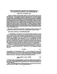
~ (i)) exist in 3 possible Figure 2. (a)~(c) are examples of G~ r ,i (w r ways, while the case (d) would not exist. Blue solid curve ~ r, i ~ ~ (i)) and red dot curve indicates G indicates G~−r,i (w r + (wr (i)).

where C r,i1 and C r,i2 are constant values independent of ~ (i ) . It thus can be verified that for fixed w r {w~c ( j),(c, j) ≠ (r,i)} and {hk(j)}, minimizing G(W,H) with ~ (i ) is equal to minimizing the following respect to w r ~ (i ) : formula with respect to w r ~ r, i ~ r, i ~ ~2(i) + br, iw ~ r, i w  G ( w ( i )) a = r r + + r (i) + C , wr (i) ≥ 0 ~ ~  G r, i (w ( i )) = (8) r  ~ r, i ~ r, i ~ r, i ~2 r, i ~ G− (wr (i)) = a wr (i) + b− wr (i) + C , wr (i) < 0 where a r , i = [∑ sN=1 h 2s (i)] ~ ( j) + β b +r , i = b 0r , i + 2 α ∑ lj =1, j ≠ i w r r, i ~ ( j) − β r i l , b − = b 0 − 2 α ∑ j = 1, j ≠ i w r ~ ( j)h ( j) − 2 ∑ N ~ b0r, i = 2 ∑kN=1 hk (i) ∑lj =1, j ≠i w r k k =1 x r (k )h k (i)

C r , i = C1r , i + C 2r, i

It is interesting to show the possible existing styles of ~ ~ (i )) in Fig. 2, where Fig. 2 (d) would not function G r , i (w r ~ ( j ) + β ≥ 0 for ever. exist because 2α ∑ lj =1, j ≠ i w r Finally, the optimal solution is given by the following lemma and theorem, and the proofs are omitted. ~ r ,i ~ b r ,i ~ + (i) = arg min ~ Lemma 1. w − 2 a+r ,i ,0) r ~wrr ,(ii )≥~0 G+ (w r (i)) = max( b−r ,i ~ − and w r (i) = arg minw~ r (i )<0 G− (w r (i)) = min(− r ,i ,0) . 2a ~ opt (i ) is the minimum Theorem 1. Suppose w solution of r ~ ~ ~ r, i ~ , r i ~+ (i)) < G r, i (w ~−(i)), and ~opt(i) = w ~ + (i) if G (w G (wr (i)) . Then w r r + r − r opt ~ ~ − otherwise. w r (i ) = w r (i ) „ Optimize h s (i ) for fixed {wj(c)} and {hk(j), (k,j)≠(s,i)} N We know ||X-WH|| 2F =Σ k=1 ||xk-Whk|| 2F . Hence for fixed {wj(c)} and {hk(j), (k,j)≠(s,i)}, minimizing G( W, H) with respect to h s (i) is equal to minimizing the formula below: ~ G s , i (h s (i )) =|| x s − Wh s ||2F + λ ∑ lj =1 h s ( j )

= h Ts W T Wh s − 2h Ts W T x s + x Ts x s + λ ∑ lj =1 h s ( j ) = ∑ nc =1 (∑ lj =1 h s ( j ) w j (c )) 2 − 2 ∑ lj =1 h s ( j )( w Tj x s ) + λ ∑ lj =1 h s ( j ) + x Ts x s = ∑ lj1 =1 ∑ lj2 =1 ∑ cn=1 h s ( j1 )h s ( j2 )w j1 (c ) w j2 (c ) − 2 ∑ lj =1 h s ( j ) w Tj x s + λ ∑ lj =1 h s ( j ) + xTs x s

(9)

~ s, i ~ s, i ~ s, i ~ s, i 2 G , h s (i ) ≥ 0 + (h s (i)) = a h s (i ) + b+ h s (i ) + C = ~ ~ ~ , s i ~ s, i 2 s, i s, i G− (h s (i)) = a h s (i ) + b− h s (i ) + C , h s (i ) < 0

where a~ s , i = [∑ nc=1 w i2 (c)]

~ b+s, i = −2wTi x s + 2 ∑lj=1, j ≠i ∑nc=1 h s ( j)w j (c)wi (c) + λ ~ b−s,i = −2wTi x s + 2 ∑lj =1, j ≠i ∑nc=1 h s ( j)w j (c)wi (c) − λ ~ C s, i is a constant independent of h s (i ) .

Without proofs, we similarly get the following conclusions. ~s , i ~ Lemma 2. h+s (i) = arg~minhs (i )≥0 G+s, i (h s (i))~= max(− 2ba~+s , i ,0) s,i , s i b and h−s (i) = argminhs (i )<0 G− (h s (i)) = min(− 2a~−s, i ,0) . Theorem 2. Suppose h opt s (i ) is the minimum solution of ~ ~ ~ opt G s , i ( h s (i )) . Then hs (i) = h+s (i) if G+s, i (h s+ (i)) < G−s, i (h −s (i)) , opt and h s (i ) = h −s (i ) otherwise. Based on the above optimization scheme of CSMF, optimization scheme of CSMFnc for minimizing Eq. (5) could be easily derived by only changing the update rule of ~ (i ) ≥ 0 , the components. First, we find that when w r ~ r, i ~ G ( w r (i)) in Eq. (8) could be reduced to: ~ ~ (i )) = a r , i w ~ 2 (i ) + b r , i w ~ (i ) + C G r , i (w r r r +

r,i

~ (i ) ≥ 0 ,w r

(10) Then the components in CSMFnc are updated as follows. ~ opt (i) is the minimum solution of Theorem 3. Suppose w r ~ r, i ~ ~ when w ( i G (w r (i)) r ) ≥ 0 . Then r, i ~ ~ ~ opt (i) = arg min ~ (11) w G r , i (w (i)) = max(− b+ ,0) r

w r (i )≥0

+

r

2 ar , i

3.2. Gentle update strategy In the last section, a locally optimal solution is obtained. However, it would highly depend on the implementation of the alternating procedure and an unsatisfied locally optimal solution may be learned. In view of this, we propose an adaptive strategy to handle the alternating process for learning a better local optimum. The proposed strategy is to select a subset of parameters either from the component part or from the coefficient part for update at each step, rather than updating all of them. We call this strategy the gentle update strategy. Algorithm 1 is an overview of the strategy and details are given as follows. „ Gentle update of components. As W can be updated by ~ ~ }Ntw constituted the update of W , at the tth step a subset {w i' j j =1 by two parts is then selected for update. For the first part, Nwt,1 indexes {~i '1 , , ~i ' N w } are cyclicly selected from {1, … ,n} t ,1 in an orderly manner from the start of the alternating process. For the second part, Nwt,2 indexes {iˆ '1 , , iˆ ' N tw, 2 } ~ ~ are selected such that the subset {G(w ), r ∈{iˆ'1 , , iˆ' Ntw, 2 }} ~ ~r w consists of the largest Nt,2 values in {G(w r ), r = 1, , n} , where ~~ ~ l l ~ ~ ~ ( j)| T~ 2 G(wr ) =|| xr −H wr ||F +α∑j1=1 ∑j2 =1, j2 ≠ j1 | wr ( j1)|| wr ( j2)| +β∑jl=1 | w r (12) ~ ~ By Eq. (6)~(7), we find that G(w r ) can fully reflect the ~ in minimization of the criterion. (Eq. contribution of w r (12) can also be used for CSMFnc). Denote the selected indexes by {i'1 , , i' Ntw } = {~i '1 , , ~i ' Ntw,1 } ∪ {iˆ'1 , , iˆ' Ntw, 2 } . Then, the first part of this subset gives the opportunity to update all parameters and the second part is to appropriately accelerate the convergence of the algorithm.

Algorithm 1. Gentle CSMF input : Data matrix : X = ( x1 , , x N ) Parameters of gentle update strategy : N 0w,1 , N 0w, 2 , N 0h,1 , N 0h, 2 Parameters of iteration : loop , ε > 0 01 . Initilaize W and H 02 . t ← 1 03 . While (t ≤ loop ) 04 Let W0 = W and H 0 = H // save old values // update W using gentle update strategy ~ 05 . W = W T ~ } N tw for update 06 . Set N tw,1 = N 0w,1 , N tw, 2 = N 0w, 2 and select the subset {w i ' j j =1 ~ w 07 . For j = 1 : N t End update w i ' j by theorem 1; ~ 08 . W = W T // update H using gentle update strategy h

09 .

Set N th,1 = N 0h,1 , N th, 2 = N 0h, 2 and select the subset {h i ′j′ } Nj=t 1 for update

10 .

For j = 1 : N th

update h i ′′j by theorem 2;

End

// see whether the iteration can be terminated 11 . If | G ( W , H ) − G ( W0 , H 0 ) |≥ ε , t ← t + 1 . Otherwise exist . 12 . End output : W , H

„ Gentle update of coefficients. Similarly, at the tth step, h there are two parts constituting a subset {h i ′j′ }Nj=t 1 for update. ~ ~ h First, N t,1 indexes {i1′′, , iN′′th,1 } are cyclicly selected from {1, , N } in an orderly manner from the start of the alternating process. Second, the rest Nht,2 indexes {iˆ1′′, , iˆN′′th, 2 } ~ are selected such that the subset {G (h s ), s ∈ {iˆ1′′, , iˆN′′th, 2 }} h consists of the largest Nt,2 values in {G~(hs ), s = 1, , N} , where ~ (13) G (h s ) =|| x s − Wh s || 2F + λ ∑ lj =1 | h s ( j ) | It is based on Eq. (9). So, for update of the coefficients, the selected index set is {i1′′, , i′N′ th } = {~i1 ′,′ , ~iN′′th,1 } ∪ {iˆ1′′, , iˆN′′ th, 2 } . For implementation of gentle update strategy, in the experiment we let Nwt,1, Nwt,2, Nht,1 and Nht,2 be constants Nw0,1, Nw0,2 , Nh0,1 and Nh0,2 respectively, being independent of t as shown in Algorithm 1. Also, we will control the algorithm by the maximum iteration number while setting ε very small. Convergence. The alternating algorithm would be converged, because G(W,H)≥0 for any W and H, and the function G will decrease after each update. So there must be a step at which | G(W, H) − G(W0 , H0 ) |< ε in Algorithm 1. Discussion. Though alternating technique is welcome for optimization of non-convex problem, however, little work is proposed for handling the alternating process. Alternating technique implemented in traditional way, for instance in our learning, will at each step first update all components and then update all coefficients. That is to set Nw0,1=n, Nw0,2=0, Nh0,1=N and Nh0,2=0 in gentle update strategy. However, our study shows handling the process is important. Due to the limited room of the paper, we can only show an example in Fig. 4 (c) that the update using the traditional way would yield an unsatisfied result. Hence, handling the alternating process is useful.

4. Theory & experiment analyses We first further interpret the sparseness in CSMF. Then experimental analysis and theoretical analysis are given on synthetic and real-world data sets in Section 4.2.

4.1. Sparseness in CSMF As we state absolute orthogonality and lasso constraints can make components or coefficients sparse, the followings theorems tell how they work and the proofs are omitted. ~+(i) →0 Theorem 3. If α→+∞ or β→+∞, then by lemma 1, w r ~ − (i) → 0 , and consequently w ~ opt (i ) → 0 in theorem 1. and w r r Theorem 4. If λ→+∞, then by lemma 2, h +s (i ) → 0 and h −s (i ) → 0 , and consequently hopt s (i)→0 in theorem 2. In applications, the sparseness could be gained without assigning large values to α, β and λ. Interestingly, both α and β could control the degree of component sparseness by theorem 3. Their differences would be analyzed later. Next, we know that CSMF is NMF when D1={W≥0}, D2={H≥0}and α=β=λ=0. However, though non-negativity is popularly used for extracting sparse features, it still lacks of mathematical interpretations when it works, when it will fail and why imposing non-negativity on components and coefficients simultaneously are preferred. We now try to give some interpretations based on the optimization scheme in Section 3. First, we develop an alternative algorithm for solving NMF within the framework of CSMF. By modifying theorem 1 and theorem 2, the update rule is as follows. Theorem 5. For D1={W≥0}, D2={H≥0} and α=β=λ=0, ~ opt (i) = w ~ + (i) = max(− b+r,i ,0) ; (2) CSMF is updated by (1) w r r ~s, i 2ar ,i b+ + hopt s (i) = hs (i) = max(− ~s, i ,0) . 2a ~ ~ opt (i ) or h opt (i) It shows when br,i+ or b+s , i is positive, w r s will be zero, yielding sparseness in components or coefficients. This interprets why non-negativity constraint ~ may yield sparseness. However, if br,i+ or b+s , i is negative, opt opt ~ w r (i ) or h s (i) will then be positive. Thus just imposing non-negativity may not be enough always. So additional constraints are used since larger positive values α, β and λ ~ would bring br,i+ and b+s , i towards positive values, where in [9] sparseness is imposed on coefficients. With similar reason, when only one-sided non-negativity is imposed, the ~ positivity of br,i+ or b+s, i seems more undetermined according to their formulas. Next section will give some more insight. As a more general model of NMF, the CSMF with non-negative components and coefficients (CSMFncc) will be used for comparison in next section. Theorem 5 is still applicable for the optimization of CSMFncc and the condition “α=β=λ=0” can be removed from the theorem.

4.2. Evaluation & analysis We discuss the impacts of different constraints in CSMF in two cases: ground truth decomposition and approximate decomposition. In the experiment, the components of all iterative algorithms are initialized with the same positive values. The coefficients of CSMF and CSMFnc are initialized as the least square solutions of the reconstruction term since non-negativity is not needed, and for NMF based methods they are randomly initialized with the same positive values. The parameters of the compared methods are tuned by trying our best or suggested by the authors.

4.2.1 Case of ground truth decomposition In ground truth decomposition, it is assumed that a group of images could be completely represented using local features without any overlapping. So experiment as well as theoretical analysis is performed on Swimmer data set [12]. It is constituted by 256 images of size 32 × 32. Each image is represented by five parts, a centered invariant part called “torso” of 12 pixels and four “limbs” of 6 pixels appear in one of 4 positions. Some images are shown in Fig. 3. So far many algorithms have been tested on this data set. However, to the best of our knowledge, ghost is still a problem and the exact 17 factors are still not factorized out.

Figure 3. Some Images in Swimmer Data Set.

„ Absolute orthogonality. In ground truth decomposition, a group of images could be completely represented by a set of sparse components w1, … ,wl with no overlapping between them. So the components should be absolutely orthogonal. Then, it is optimistic to only use absolute orthogonality for extraction of sparse features and get the same reconstruction performance as PCA. It is because when β=λ=0 for any α>0, if absolute orthogonality is satisfied, we have: 2 2 G ( W, H ) = X − WH F + g1 ( W ) + g 2 ( H) = X − WH F . (14) In the experiment, when α=0.05, β=λ=0, Nw0,1=600, Nw0,2=200, N h0,1 =200 and N h0,2 =100, CSMF extracts all the proper components as shown in Fig. 4(a) and the difference of MSE (mean square error) results between CSMF and PCA is 1.4×10−29. Moreover, in Fig. 4(e), we see absolute orthogonality is also useful for CSMFnc, where parameter setting for update is: Nw0,1=200, Nw0,2=100, Nh0,1=100 and Nh0,2=50. „ Lasso ||W||1 Constraint. As analyzed in theorem 3, ||W||1 can also be used to control the sparseness of a component, and as shown in Fig. 4 (b) all the proper components are also extracted. In ground truth experiment, the differences between ||W||1 and the absolute orthogonality in theory are: (1). Absolute orthogonality measures the redundancy (overlapping) between components while ||W||1 only measures the average cardinality of each component. (2). In the optimistic case when global optimum is achieved, the learned components with absolute orthogonality penalty are also the best for reconstruction. The ones using constraint ||W||1 is not sure, since G(W,H)>||X-WH||2F for β>0. „ Lasso ||H||1 Constraint. To our surprise, in the ground truth decomposition as analyzed above, ||H||1 is not required to find all the proper components. However ||H||1 in CSMFnc is useful sometimes for learning sparse codings as exemplified in Section 2.2, and as seen later ||H||1 is helpful for extraction of sparse components on real-world data set. „ Non-negativity. The experiment of NMF on Swimmer was reported [13] and it is known NMF can not remove the ghost between components. Here we implement its three well-known variants, nsNMF, LNMF and NMFsc, where the parameters of nsNMF and NMFsc have been tuned by our best. The tuned parameter of nsNMF is not the same as

(a) CSMF (λ=0,α=0.05,β=0)

(b) CSMF (λ=0,α=0,β=1)

(c) Over-learned CSMF (λ=0,α=0.05,β=0)

(d) CSMF (λ=0.1,α=0.01,β=0.01)

(e) CSMFnc, (λ=0,α=0.01,β=0)

(f) CSMFnc, (λ=0.01,α=0.01,β=0.01)

(g) LNMF

(h) NMFsc (0.9,0.4)

(i) nsNMF (θ=0.1)

Figure 4. Experiment on Swimmer. (1) For CSMF, its absolute images are shown so that the more the darker pixels are the sparser the component is; (2) Dark pixels are for (almost) zero entries and white pixels are for positive ones; (3) The maximum iteration number in all methods is 2000; (4) For NMFsc, the parameters of controlling the component and coefficient sparseness are 0.9 and 0.4 respectively; for nsNMF, θ is defined in [13]; (5) See text for the parameter settings of CSMF and CSMFnc; (6) (c) is discussed at the end of Section 3.

the one reported in [13] since the initialization is different. The results in Fig. 4 show a ghost depicting the “torso” exists in each component learned by the variants of NMF. Finally, Fig. 4(d) additionally shows the result of CSMF with λ=0.1, α=0.01, β=0.01 and Nw0,1=600, Nw0,2=200, Nh0,1=150 and Nh0,2=50, and Fig. 4(f) shows the results of CSMFnc with λ=0.01, α=0.01, β=0.01 and Nw0,1=600, Nw0,2=200, Nh0,1=150 and N h0,2 =50. So, success of CSMF is not restricted to one specific parameter setting. Summary. (1) While lasso penalty has been widely used for constraint on generic data, in CSMF we introduce the absolute orthogonality penalty and justify its usefulness in ground truth experiment; (2) While non-negativity is popularly used as constraint for extraction of sparse components, CSMF and CSMFncc show constraints using absolute orthogonality and lasso penalties are also useful for matrix factorization to achieve this goal. Moreover, they help further remove the ghost and extract all proper components, while non-negative constraint may not do that. 4.2.2 Case of approximate decomposition Unlike the ground truth experiment, there is no strong evidence that a group of face images could be completely represented using (a few) limited sparse components. However approximate decomposition with sparse components is still welcome. For evaluation, we first define the average overlapping degree (AOD) between components by the following formula: AOD ( W ) = [0.5 ⋅ l ⋅ (l − 1)] −1 ∑ lr−=11 ∑ lr '=r +1 w Tr w r ' (15)

[

]−1

where wr (i) = ∑ni=1 | wr (i) | ⋅ | wr (i) | . We see that AOD(W) is a normalized absolute orthogonality measurement. If there is no overlapping between components, AOD(W) is zero. Otherwise it shall be large, with maximum value being 1.

Experiment are performed on the training set of CBCL1 [5] constituted by 2429 face images of size 19 × 19 . The pixel values of images are ranging from 0 to 1. In the experiment, 49 components are found. For convenience of analysis, the parameters of gentle update strategy are fixed and indicated in Fig. 5. First we investigate the effects of absolute orthogonality and lasso constraints on extraction of sparse components without the non-negativity constraint, i.e., D1={W∈ ℜn×l } and D2={H ∈ ℜl×N } in CSMF. Table 1 and 2 show the impact of lasso penalty on coefficients in extraction of sparse components, where either absolute orthogonality or lasso penalty on components is used; table 3 and 4 show the impacts of absolute orthogonality and lasso penalty on components respectively when no penalty is imposed on coefficients. As shown, using lasso ||H||1 as constraint is good for extracting sparse features on real-world data, though in ground truth experiment, it may not be needed. From table 1 to 3 we see that using absolute orthogonality penalty could accelerate the process of producing sparse features, while in table 4 using lasso constraint on components seems less effective. This can be further shown by table 2 as compared to table 1. However, we find that larger α would be easier to get AOD(W)=NaN. It indicates there are some over-learned components, which are (almost) −1 empty, because [∑ni=1 | wr (i) |] →+∞. In this case, one can set α properly large and then go on producing sparser components by further increasing β and λ as shown in table 5. Next, we investigate the effect of non-negativity constraint and its differences from other constraints. First, 1 No preprocessing is done on CBCL here, while some preprocessing, such as removing mean, clipping etc, are first applied by Lee [1] and Hoyer [8] in their codes (it is not clear in [13]). The preprocessing may perform some nonlinear transform on the data.

α=0.1

λ=0 0.35187

λ=0.01 0.27679

λ=0.05 0.17524

λ=0.08 0.13023

λ=0.1 0.11722

λ=0.3 0.05768

λ=0.5 NaN

Table 1.Impact of Lasso (||H||1) Constraint, β=0, AOD(W) β=0.01 β=0.1

α=0 0.63806 0.52735

α=0.01 0.44284 0.42875

α=0.05 0.37664 0.37435

α=0.08 0.37208 0.36906

α=0.1 0.35124 0.3478

α=0.2 0.32024 0.31461

α=0.3 NaN NaN

Table 3.Impact of Absolute Orthogonality, λ=0, AOD(W) β=0.1

λ=0.05 0.16034

λ=0.1 0.11655

λ=0.2 0.07082

λ=0.05 0.14251

β=0.5

λ=0.1 0.1077

λ=0.2 0.06892

β=0.1

λ=0 λ=0.01 0.52735 0.51248

λ=0.05 0.46932

λ=0.08 0.4466

λ=0.1 0.43335

λ=0.3 0.35167

λ=0.5 0.31272

Table 2. Impact of Lasso (||H||1) Constraint, α=0, AOD(W) α=0.01 α=0.1

β=0 β=0.01 β=0.05 β=0.08 β=0.1 β=0.2 0.44486 0.44284 0.43606 0.43101 0.42875 0.42081 0.35187 0.35124 0.35053 0.34928 0.3478 0.34159

β=0.3 0.41248 0.34049

Table 4. Impact of Lasso (||W||1) Constraint, λ=0, AOD(W) β=1

λ=0.05 0.13026

λ=0.1 0.08478

λ=0.2 0.06538

β=1.5

λ=0.05 0.1028

λ=0.1 0.07391

λ=0.2 NaN

Table 5. Impact of Lasso Constraints, α=0.1, AOD(W)

we give some visual results in Fig. 5. In the first four columns, non-negativity is gradually imposed in CSMF. It is imposed on components in the second row and on both components and coefficients in the third row. Note that in Fig. 5(k), CSMFncc is actually the NMF implemented by theorem 5. We see that non-negativity helps produce sparse components as supported by theorem 5. However, when non-negativity is imposed on components and coefficients simultaneously, it shows that the ghosts in some components are hard to be removed and also further incorporating other constraints is not effective to alleviate the overlapping between components, since there is no apparent difference among Fig. 5(k), Fig. 5(l) and Fig. 5(m). With further results shown in table 6 when non-negativity is imposed on both components and coefficients, AOD(W) only changes a little when other constraints are used. In contrast, AOD(W) changes obviously in table 3 and 4. Moreover, in the third row and fourth column CSMFncc is over-learned. This may be due to the improperly large weights of the constraints. As some more results of CSMFncc are shown in Fig. 6 with different parameter settings, it can still show that no significant change exhibits. On the other hand, when non-negativity is not simultaneously imposed on components and coefficients, the components become sparser when absolute orthogonality and lasso constraints are further imposed as shown from Fig. 5(a) to Fig. 5(d) and from Fig. 5(f) to Fig. 5(i). Very interestingly, using lasso constraint ||H||1 could further remove the ghost in the components. Finally, besides the example shown in Section 2, to see the further advantage of allowing subtraction of nonnegative sparse components, we tabulate the MSE results corresponding to the visual results in Fig. 5 and Fig. 6 on CBCL in table 7. Compared to NMF [1], CSMFnc can produce much sparser (more localized) features while lower MSE values can be gained. Note that the MSE of λ=0, α=0.1 λ=0, β=0.1

β=0.01 0.18287 α=0.01 0.18433

β=0.05 0.18283 α=0.05 0.18355

β=0.1 0.18144 α=0.1 0.18144

β=0.2 0.18015 α=0.2 0.17384

β=0.3 0.17445 α=0.3 0.17012

Table 6. Impact of Constraints, with Non-negativity, AOD(W) Method

MSE

CSMF (λ=0,α=0,β=0) 0.61576 CSMFncc(λ=0.001,α=0.05,β=0.05) 0.75877 CSMFncc(λ=0.001,α=0.01,β=1) 0.76322 CSMFncc (λ=0.001,α=0.1,β=0.001) 0.7575 CSMFncc (λ=0,α=0,β=0) 0.76566 NMFsc (0.8, 0) [8] 1.3577 nsNMF (θ=0.6) [14] 1.5578

Method

MSE

CSMFnc (λ=0,α=0,β=0) CSMFnc (λ=0.05,α=0.1,β=1) CSMFnc (λ=0.1,α=0.05,β=1) CSMFnc (λ=0.2,α=0.1,β=1) NMF [3] (Euclidean distance) LNMF [11] PCA

0.6157 0.70183 0.74385 0.85249 0.8631 5.051 0.60871

Table 7. Reconstruction Errors on CBCL

CSMFnc with λ=0.05, α=0.1 and β=1 is 0.70183, while NMF is 0.8631 and CSMFncc is 0.76566. Though nsNMF is motivated for pursuing sparseness in both components and coefficients, however Fig. 5(i) is sparser than Fig. 5(o) with smaller MSE. Though LNMF and NMFsc can extract sparser features, their MSEs are high, being 5.051 and 1.3577 respectively. In fact there should be some trade-off between sparseness and reconstruction ability. Moreover, in Fig. 4 LNMF and NMFsc can not remove the ghost. So, allowing both additive and subtractive combinations of a set of non-negative sparse components may be more useful for representation of complex object in a more accurate way. Summary. (1) Absolute orthogonality can accelerate the process of producing sparse components; (2) Lasso constraint ||H||1 helps remove ghost in the components; (3) Non-negativity is useful, but it seems hard to deal with the ghost problem; (4) Subtractive combination of non-negative sparse components may be good for a trade-off between sparseness and lower MSE value.

5. Conclusions In this paper, the impacts of different constraints for pursuing sparse components and the relationship among them are theoretically and experimentally analyzed in the framework called Constrained Sparse Matrix Factorization (CSMF). The conditions when non-negativity constraint is useful for extraction of sparse components are investigated. It is also found that subtractive combination of non-negative sparse components is effective. Moreover, a gentle update strategy, as a useful technique for pursuing a better local optimum, is suggested for the optimization in CSMF. The proposed model has been finally justified to be effective for elimination of the ghost between components. In future, we will further consider the impacts of different constraints for pursuing sparse components in the aspect of classification.

6. Acknowledgements This work was supported by NSFC (60675016, 60633030), 973 Program (2006CB303104) and NSF of GuangDong (06023194).

References [1]. D. D. Lee and H. S. Seung. Learning the parts of objects by non-negative matrix factorization. Nature, 401: 788–791, 1999.

(a) CSMF, λ=0,α=0,β=0

(b) CSMF, λ=0,α=0.1,β=0

(c) CSMF, λ=0,α=0.1,β=1

(d) CSMF, λ=0.2,α=0.1,β=1

(e) LNMF

(f) CSMFnc, λ=0,α=0,β=0

(g) CSMFnc, λ=0,α=0.1,β=0

(h) CSMFnc, λ=0,α=0.1,β=1

(i) CSMFnc, λ=0.2,α=0.1,β=1

(j) NMFsc (0.8,0)

(k) CSMFncc, λ=0,α=0,β=0

(l) CSMFncc, λ=0,α=0.1,β=0

(m) CSMFncc, λ=0,α=0.1,β=1

(n) CSMFncc, λ=0.2,α=0.1,β=1

(o) nsNMF (θ=0.6)

Figure 5. Experiment on CBCL. See text for detailed analysis. Setting: (1) For CSMFnc and CSMFncc, white pixels denote (almost) zero gray value and darker ones denote positive gray values; (2) The maximum iteration in all algorithms is 1000; (3) Figures of CSMF are shown as their absolute images, so the less the dark pixels are the sparser the component is. (The roles of the white and dark pixels here are different from those in Fig. 4 because of the traditional use for visualization); (4) Parameters of NMFsc are suggested in [8]; (5) The parameter setting of the gentle update strategy for CSMF, CSMFnc and CSMFncc is: Nw0,1=100, Nw0,2=50, Nh0,1=300 and Nh0,2=100. [2]. R. Zass and A. Shashua. Nonnegative Sparse PCA. NIPS 2006. [3]. D. D. Lee and H. S. Seung. Algorithms for non-negative matrix factorization. NIPS, 2000. [4]. P. S. Penev and J. J. Atick. Local feature analysis: a general statistical theory for object representation. Network: Computation in Neural Systems, 7(3): 477-500, 1996. [5]. MIT Center for Biological and Computation Learning, CBCL Face Database #1, http://www.ai.mit.edu/projects/cbcl. [6]. M. D. Plumbley. Algorithms for non-negative independent component analysis. IEEE TNN, 14(3): 534-543, 2003. [7]. H. Park and H. Kim. One-sided non-negative matrix factorization and non-negative centroid dimension reduction for text Classification. Proc. of the 4th Workshop on Text Mining, SDM 2006. [8]. P.O. Hoyer. Non-negative matrix factorization with sparseness constraints. JMLR, 5: 1457-1469, 2004. [9]. P.O. Hoyer. Nonnegative Sparse Coding. Proc. IEEE

Workshop Neural Networks for Signal Processing, 2002. [10]. Hyvärinen, J. Karhunen, and E. Oja. Independent Component Analysis. John Wiley and Sons, 2001. [11]. S. Z. Li, X. Hou, H. Zhang, and Q. Cheng. Learning spatially localized parts-based representations. CVPR, 2001. [12]. D. Donoho and V. Stodden. When does non-negative matrix factorization give a correct decomposition into parts? NIPS, 2003. [13]. A. Pascual-Montano, J. M. Carazo, K. Kochi, D. Lehmann, and R. D. Pascual-Marqui. Nonsmooth non-negative matrix factorization (nsNMF). IEEE TPAMI, 28(3): 403-415, 2006. [14]. H. Zou, T. Hastie, and R. Tibshirani, “Sparse principal component analysis,” Technical Report, Statistics Department, Stanford University, 2004. [15]. M. Kirby and L. Sirovich. Application of the karhunenloeve procedure for the characterization of human faces. IEEE TPAMI, 12(1): 103-108, 1990.

(a) CSMFnc, λ=0.05,α=0.1,β=1 (b) CSMFnc, λ=0.1,α=0.05,β=1 (c) CSMFncc, λ=0.001,α=0.05,β=0.05 (d) CSMFncc, λ=0.001,α=0.01,β=1 (e) CSMFncc, λ=0.001,α=0.1,β=0.001

Figure 6. More results of CSMFnc and CSMFncc on CBCL (other parameter settings are the same as Fig. 5).