The 7th International Conference on Ubiquitous Robots and Ambient Intelligence (URAI 2010)
Numerical Solutions to Relative Pose Problem under Planar Motion Sunglok Choi, JaeYeong Lee, Ji Hoon Joung, M. S. Ryoo, and Wonpil Yu Robot Research Department, ETRI, Daejeon, Republic of Korea {sunglok, jylee, jihoonj, mryoo, ywp}@etri.re.kr
Abstract— In this paper, we propose a novel solution to relative pose problem under planar motion. Planar motion is common in indoor and on-road situation, and it can be approximated as circular in small movement. We use two levels of motion, planar and planar circular motion, as prior to derive the solution. Moreover, two levels of motion are applied to two different geometric models: an essential matrix and planar homography. Therefore, this paper deals with four combinations of solution to relative pose problem. We can estimate relative pose using less number of point correspondence with the motion prior. For example, five pairs of points are necessary to estimate an essential matrix, but only two points are enough to deduce an essential matrix under planar motion. In addition, our solution is much faster than ordinary methods with more correspondence.
Fig. 1. Three levels of motions from 1st camera to 2nd camera: red denotes parameters which describe each motion.
Keywords— Relative Pose Problem, Planar Motion, Essential Matrix, Planar Homography, 1-Point RANSAC
1. Introduction Relative pose problem is to estimate relative movement between a pair of images. It is one of the classical problems in computer vision, and their solutions are also well-known [1]. Two geometric models, essential matrix and planar homography, are representative forms to describe such relative pose. They are usually estimated by point correspondence, a pair of matched points. Four pairs of points decide a planar homography, which is decomposed to two physically possible solutions. Similarly, five correspondences entail an essential matrix, which is decomposed to one physically possible solution. Estimating an essential matrix has been studied until recently [2], [3], [4]. The core of 1-point RANSAC [5] is to estimate an essential matrix from single correspondence. It was proposed in robotics field to reject incorrect correspondence in real-time structure from motion [5], [6]. It is much faster than plain RANSAC with five-point algorithm because it uses only one point. RANSAC requires exponentially more iterations according to the necessary number of points in generating a hypothesis (e.g. an essential matrix). Two kinematic constraints enable single point to estimate an essential matrix. The first constraint is planar motion. If a camera mounted on a vehicle moves on a corridor or road, it undergoes planar motion. It is a quite common situation in indoor and on-road as shown in Figure 2. The second constraint This work was supported partly by the R&D program of the Korea Ministry of Knowledge and Economy (MKE) and the Korea Evaluation Institute of Industrial Technology (KEIT). (The Development of Low-cost Autonomous Navigation Systems for a Robot Vehicle in Urban Environment, 10035354)
Fig. 2.
Two examples of planar motion: indoor (left) and on-road (right)
is circular motion. If a piecewise movement is small, the motion can be approximated as circular. However, previous works [5], [6] only concentrated on an essential matrix, not planar homography. They proposed an algebraic solution to 1-point problem (under planar circular motion), but they used iterative optimization to 2-point problem (under planar motion). In this paper, we derives two geometric models (essential matrix and planar homography) under two levels of motion (planar and planar circular motion). We also propose numerical solutions to estimate them. Our works consider relative pose problem using planar homography. Moreover, our numerical solution are much faster and simpler than the previous work [7]. 2. Reduced Geometric Models We follows the conventional coordinate utilized in computer vision as shown in Figure 3. 2.1 Planar and Circular Motion An object under planar motion moves parallel to a plane. For example, a vehicle on a road undergoes planar motion. The vehicle keeps the constant interval from the road when
The 7th International Conference on Ubiquitous Robots and Ambient Intelligence (URAI 2010)
A reduced essential matrix under planar motion is 0 cos(θ − φ ) 0 0 sin φ , E = ρ − cos φ 0 sin(θ − φ ) 0
(7)
which comes from (1) and (5). It is represented by only two parameters, θ and φ . The essential matrix under planar motion cannot describe the magnitude of translation, ρ. Fig. 3. A point is observed at two image frames. The image coordinate is located at its top-left. The metric coordinate is at the center of camera.
it moves. The planar motion has 3 degree of freedom (DoF) as like [x, y, θ ]T or [ρ, φ , θ ]T . One is rotation on the plane, and the other two is translation on the plane. If the principal axis of a camera is parallel to the plane, the rotation and translation of the camera are described as follows: cos θ 0 sin θ sin φ 1 0 and T1 = ρ 0 , (1) R21 = 0 − sin θ 0 cos θ cos φ where R21 is rotation of the 2nd image frame with respect to the 1st image frame, and T1 is translation of the 2nd image frame with respect to the 1st frame as shown in Figure 1(b). An object under circular motion moves around a point with constant radius. If we split general motion into small piece, each piecewise motion can be approximated as circular motion. As an extreme example, straight motion is regarded as piecewise circular with infinitely long radius. In circular motion on a plane, its rotation and translation have relation as follows: θ = 2φ , (2) which is simply verified from Figure 1(c). This relation makes planar circular motion have 2 DoF. In general, a point in 3D space can be observed as xˆ 1 and xˆ 2 in the 1st and 2nd images, respectively. A pinhole camera model restores each point from pixel unit to metric unit as follows: x1 = K1−1 xˆ 1 and x2 = K2−1 xˆ 2 , (3) where Ki is ith camera matrix. In general, two calibrated points are correlated with relative pose as follows: x2 = R12 x1 + T2 ,
(4)
where R12 is rotation of the 1 image frame with respect to T T the 2nd image frame, R21 , and T2 is translation as −R21 T1 . The relation deduces definition of an essential matrix (5) and planar homography (8), which is described in [1], [8]. 2.2 Reduced Essential Matrix An essential matrix is a 3-by-3 matrix defined as follows: E = [T2 ]× R12 ,
(5)
where [T2 ]× is matrix representation of cross product with T2 . An essential matrix satisfies the following condition with a pair of matched points: xT2 Ex1 = 0 .
(6)
2.3 Reduced Planar Homography of Ground Plane A planar homography is a 3-by-3 matrix defined as follows: � 1 H = λ R12 + T2 N T , (8) d where λ is a scaling parameter, N is a normal vector of a plane where correspondence exists, and d is distance from a camera to the plane. A planar homography satisfies the following condition with a pair of matched points: x2 = Hx1 ,
(9)
where two points, x1 and x2 , should be on the same plane by definition. A reduced planar homography under planar motion is ρ − sin θ cos θ d sin(θ − φ ) 1 0 , (10) H =λ 0 ρ sin θ − d cos(θ − φ ) cos θ which comes from (1) and (8). It is represented by five parameters: λ , d, ρ, θ , and φ . Our reduced planar homography (10) assumes that the given plane is the ground surface, N = [0, 1, 0]T . Actually, the reduced homography is not necessary to limit its plane to the ground. If we permit an arbitrary plane, the reduced planar homography (10) becomes complex similarly with an ordinary planar homography. Such complex reduced homography does not take advantage of reduced models which are able to be estimated by less number of correspondence. Moreover, if we assume the given plane as the ground surface, distance parameter d is constant during planar motion. The known parameter d solves the scale ambiguity of relative pose, which can be one more advantage of planar homography of the ground plane. 3. Relative Pose Estimation using Reduced Geometric Models We present numerical solutions to estimate an essential matrix and planar homography. Each model is tacked as twopoint method (under planar motion) and one-point method (under planar circular motion), respectively. Figure 4 describes their number of solutions. 3.1 Reduced Essential Matrix A reduced essential matrix has a constraint with a pair of points, [x1 , y1 , z1 ]T and [x2 , y2 , z2 ]T , as follows: z1 x1 z2 x2 sin φ − cos φ + sin(θ − φ ) + cos(θ − φ ) = 0 , y1 y1 y2 y2 (11)
The 7th International Conference on Ubiquitous Robots and Ambient Intelligence (URAI 2010)
where (2i − 1)th and (2i)th row of A is and b are � � � � x1 y2 −z1 y2 0 y1 y2 x2 y1 Ai = and bi = , (19) z1 y2 x1 y2 −y1 y2 0 z2 y1 Fig. 4. This table presents three levels of motions, their DoF, and their number of solutions. Especially, N means the necessary numbers of correspondence. M means the number of algebraic solutions, and P means the number of physically possible solutions.
which comes from (6) and (7). Two-Point Algorithm The constraint (11) contains two unknowns, θ and φ , so more than two correspondences can solve it. It is formulated as follows: � � � � sin φ sin(θ − φ ) Aa = Bb such that a = , b= , (12) cos φ cos(θ − φ ) where ith row of A and B are � � � � Ai = z1 y2 , −x1 y2 and Bi = − z2 y1 , −x2 y1 ,
(13)
which comes from ith correspondence. The linear equation is also represented as a = A−1 Bb = Cb .
(14)
It is apparent that ||a|| = 1, ||b|| = 1, and ||Cb|| = 1. Finally, we can get b from the system of quadratic equations as follows: bT CT Cb = 1 and bT b = 1 . (15) We can also retrieve the other unknown a from (14) with known b. One-Point Algorithm One correspondence is enough with the planar circular constraint, θ = 2φ . From (11), φ is simply solved as follow: φ = tan−1
±(x2 y1 − x1 y2 ) . ∓(z2 y1 + z1 y2 )
(16)
The solution is same with Scaramuzza et. al. [5], [7]. 3.2 Reduced Plannar Homography of Ground Plane A reduced ground plane homography has a constraint with a pair of points, [x1 , y1 , z1 ]T and [x2 , y2 , z2 ]T , as follows: x2 x1 z1 ρ = cos θ − sin θ + sin(θ − φ ) y2 y1 y1 d z2 x1 z1 ρ = sin θ + cos θ − cos(θ − φ ) , y2 y1 y1 d
(17)
which comes from (9) and (10). Two-Point Algorithm The constraint (17) contains three unknowns, ρ, θ , and φ , so more than two correspondences can solve it. They are formulated as follows: cos θ sin θ Aa = b such that a = (18) ρ cos(θ − φ ) , d ρ d sin(θ − φ )
which comes ith correspondence. The linear equation is simply solved as a = A−1 b. One-Point Algorithm One correspondence is enough with the planar circular constraint, θ = 2φ . Interestingly, φ is derived as the same from with (16).
4. Experiments Configuration We performed Monte Carlo experiment to measure accuracy of each algorithm. Two image frames were observed, and the second image frame was apart from the first image frame as much as [ρ, φ , θ ]T = [1.5, 0.39, 0.78]T ,
(20)
whose units are meter and radian. Two-point algorithms used two pairs of matched points, and one-point algorithms used single pair of points. A point in 3D space was randomly generated on the ground plane which is d = 1.5 meters below the camera. The point was observed on 2D image plane through the ideal perspective camera model whose camera matrix is known as follows: 100 0 320 K = 0 100 240 . (21) 0 0 1 Each point on the image plane had varying magnitude of Gaussian noise from σ = 0 to σ = 2. Each algorithm was performed 103 times for statistically meaningful results. Results and Discussion One-point algorithms were more accurate than their two-point version as shown in Figure 5. Moreover, one-point algorithms utilized single correspondence, that is, less number of correspondence than two-point algorithms. It may result from less DoF by circular motion prior. In other words, one-point algorithms deal with much smaller solution space than their two-point version. It makes one-point algorithm more stable in varying magnitude of noise. Similarly, we expect that two-point algorithms will have higher accuracy than their five-point and four-point version which deal with 6 DoF problem. Two geometric models had quite similar accuracy as shown in Figure 5. A reduced planar homography involves more prior such that all correspondences are on the same plane. The reduced planar homography also accompanies with more parameters such as ρ, d, and λ . These enable twopoint algorithm of the reduced homography to be simpler and faster than two-point algorithm of the reduced essential matrix. Moreover, these can solve the scale ambiguity with known d. We believe that the reduced planar homography has merits even though it requires correspondence on the same plane.
The 7th International Conference on Ubiquitous Robots and Ambient Intelligence (URAI 2010)
References
(a) A reduced essential matrix
(b) A reduced planar homography of the ground plane Fig. 5.
A histogram of estimated φ by two reduced geometric models
5. Conclusion In this paper, we introduce two reduced version of geometric models: an essential matrix and planar homography. We also derive their numerical solution under planar and planar circular motion. In our experiments, two reduced geometric models had similar accuracy, but they have strength and weakness. The reduced planar homography has simpler and faster two-point algorithm without scale ambiguity. However, it needs correspondence on the same plane, not arbitrary points on 3D space. As further works, we will investigate two reduced models more as follows: • • • • • •
Derive two reduced models in general camera pose, not a camera aligned horizontally Derive the reduced planar homography which does not assume the ground plane. Derive a numerical solution of the above novel reduced homography. Follow one-point algorithms in least-square sense [7]. Compare their accuracy and computing time with their 6 DoF algorithms (five-point and four-point algorithms). Analysis each algorithm in various configuration, not only Gaussian noise on observation.
Moreover, we will apply our proposed algorithms to on-road visual odometry.
[1] R. Hartley and A. Zisserman, Multiple View Geometry in Computer Vision, 2nd ed. Combridge, 2003. [2] D. Nister, “An efficient solution to the five-point relative pose problem,” IEEE Transactions on Pattern Analysis and Machine Intelligence (TPAMI), vol. 26, no. 6, pp. 756–770, 2004. [3] H. Stewenius, C. Engels, and D. Nister, “Recent developments on direct relative orientation,” ISPRS Journal of Photogrammetry and Remote Sensing, vol. 60, no. 4, pp. 284–294, June 2006. [4] H. Li and R. Hartley, “Five-point motion estimation made easy,” in Proceedings of International Conference on Pattern Recognition (ICPR), 2006. [5] D. Scaramuzza, F. Fraundorfer, and R. Siegwart, “Real-time monocular visual odometry for on-road vehicles with 1-point RANSAC,” in Proceedings of IEEE International Conference on Robotics and Automation (ICRA), 2009. [6] J. Civera, O. G. Grasa, A. J. Davison, and J. M. M. Montiel, “1-point RANSAC for EKF-based structure from motion,” in Proceedings of IEEE/RSJ International Conference on Intelligent Robots and Systems (IROS), 2009. [7] D. Scaramuzza, F. Fraundorfer, M. Pollefeys, and R. Siegwart, “Absolute scale in structure from motion from a single vehicle mounted camera by exploiting nonholonomic constraints,” in Proceedings of IEEE International Conference on Computer Vision (ICCV), 2009. [8] Y. Ma, S. Soatto, J. Kosecka, and S. S. Sastry, An Invitation to 3-D Vision: From Images to Geometric Models. Springer, 2004.