PHYSICAL REVIEW A 76, 022510 共2007兲
Nuclear spin effects in optical lattice clocks Martin M. Boyd, Tanya Zelevinsky, Andrew D. Ludlow, Sebastian Blatt, Thomas Zanon-Willette, Seth M. Foreman, and Jun Ye JILA, National Institute of Standards and Technology and University of Colorado, Department of Physics, University of Colorado, Boulder, Colorado 80309-0440, USA 共Received 6 April 2007; published 29 August 2007兲 We present a detailed experimental and theoretical study of the effect of nuclear spin on the performance of optical lattice clocks. With a state-mixing theory including spin-orbit and hyperfine interactions, we describe the origin of the 1S0- 3 P0 clock transition and the differential g factor between the two clock states for alkaline-earth-metal共-like兲 atoms, using 87Sr as an example. Clock frequency shifts due to magnetic and optical fields are discussed with an emphasis on those relating to nuclear structure. An experimental determination of the differential g factor in 87Sr is performed and is in good agreement with theory. The magnitude of the tensor light shift on the clock states is also explored experimentally. State specific measurements with controlled nuclear spin polarization are discussed as a method to reduce the nuclear spin-related systematic effects to below 10−17 in lattice clocks. DOI: 10.1103/PhysRevA.76.022510
PACS number共s兲: 32.10.Fn, 42.62.Eh, 32.60.⫹i, 42.62.Fi
Optical clocks 关1兴 based on alkaline-earth-metal 共atoms兲 confined in an optical lattice 关2兴 are being intensively explored as a route to improve state of the art clock accuracy and precision. Pursuit of such clocks is motivated mainly by the benefits of Lamb-Dicke confinement which allows high spectral resolution 关3,4兴 and high accuracy 关5–8兴 with the suppression of motional effects, while the impact of the lattice potential can be eliminated using the Stark cancellation technique 关9–12兴. Lattice clocks have the potential to reach the impressive accuracy level of trapped ion systems, such as the Hg+ optical clock 关13兴, while having an improved stability due to the large number of atoms involved in the measurement. Most of the work performed thus far for lattice clocks has been focused on the nuclear-spin induced 1S0- 3 P0 transition in 87Sr. Recent experimental results are promising for development of lattice clocks as high performance optical frequency standards. These include the confirmation that hyperpolarizability effects will not limit the clock accuracy at the 10−17 level 关12兴, observation of transition resonances as narrow as 1.8 Hz 关3兴, and the excellent agreement between high accuracy frequency measurements performed by three independent laboratories 关5–8兴 with clock systematics associated with the lattice technique now controlled below 10−15 关6兴. A main effort of the recent accuracy evaluations has been to minimize the effect that nuclear spin 共I = 9 / 2 for 87Sr兲 has on the performance of the clock. Specifically, a linear Zeeman shift is present due to the same hyperfine interaction which provides the clock transition, and magnetic subleveldependent light shifts exist, which can complicate the stark cancellation techniques. To reach accuracy levels below 10−17, these effects need to be characterized and controlled. The long coherence time of the clock states in alkalineearth-metal共atoms兲 also makes the lattice clock an intriguing system for quantum information processing. The closed electronic shell should allow independent control of electronic and nuclear angular momenta, as well as protection of the nuclear spin from environmental perturbation, providing a robust system for coherent manipulation 关14兴. Recently, protocols have been presented for entangling nuclear spins in 1050-2947/2007/76共2兲/022510共14兲
these systems using cold collisions 关15兴 and performing coherent nuclear spin operations while cooling the system via the electronic transition 关16兴. Precise characterization of the effects of electronic and nuclear angular-momentum-interactions and the resultant state mixing is essential to lattice clocks and potential quantum information experiments, and therefore is the central focus of this work. The organization of this paper is as follows. First, state mixing is discussed in terms of the origin of the clock transition as well as a basis for evaluating external field sensitivities on the clock transition. In the next two sections, nuclear-spin related shifts of the clock states due to both magnetic fields and the lattice trapping potential are discussed. The theoretical development is presented for a general alkaline-earth-metal-type structure, using 87Sr only as an example 共Fig. 1兲, so that the results can be applied to other species with similar level structure, such as Mg, Ca, Yb, Hg, Zn, Cd, Al+, and In+. Following the theoretical discussion is a detailed experimental investigation of these nuclear spin related effects in 87Sr, and a comparison to the theory sections. Finally, the results are discussed in the context of the performance of optical lattice clocks, including a comparison with recent proposals to induce the clock transition using external fields in order to eliminate nuclear spin effects 关17–22兴. The Appendix contains additional details on the state mixing and magnetic sensitivity calculations. I. STATE MIXING IN THE ns np CONFIGURATION
To describe the two-electron system in intermediate coupling, we follow the method of Breit and Wills 关23兴 and Lurio 关24兴 and write the four real states of the ns np configuration as expansions of pure spin-orbit 共LS兲 coupling states,
022510-1
兩 3 P0典 = 兩 3 P00典, 兩 3 P1典 = ␣兩 3 P01典 + 兩 1 P01典, 兩 3 P2典 = 兩 3 P02典, ©2007 The American Physical Society
PHYSICAL REVIEW A 76, 022510 共2007兲
BOYD et al.
(5 s 5 p )1P1
state can also be written as a combination of pure states using Eq. 共1兲,
7 2 11 2 9 2
5
�, �
�0
13
�0
State Mixing LS HFI
7
461
�0 689
9
698
(5 s 2 )1S 0
9
2
2
11
State 3P 1 3P 2 1P 1
2
2
2
兩 3 P0典 = 兩 3 P00典 + 共␣0␣ − 0兲兩 3 P01典 + 共␣0 + 0␣兲兩 1 P01典
(5 s 5 p ) 3P2
+ ␥0兩 3 P02典.
2
The HFI mixing enables a nonzero electric-dipole transition via the pure 1 P01 state, with a lifetime which can be calculated given the spin-orbit and HFI mixing coefficients, the 3 P1 lifetime, and the wavelengths 共兲 of the 3 P0 and 3 P1 transitions from the ground state 关39兴,
(5 s 5 p ) 3P1
(5 s 5 p ) 3P0 A(MHz) -260 -212 -3.4
Q(MHz) -35 67 39
FIG. 1. 共Color online兲 Simplified 87Sr energy level diagram 共not to scale兲. Relevant optical transitions discussed in the text are shown as solid arrows, with corresponding wavelengths given in nanometers. Hyperfine structure sublevels are labeled by total angular momentum F, and the magnetic dipole 共A兲 and electric quadrupole 共Q, equivalent to the hyperfine B coefficient兲 coupling constants are listed in the inset. State mixing of the 1 P1 and 3 P1 states due to the spin-orbit interaction is shown as a dashed arrow. Dotted arrows represent the hyperfine induced state mixing of the 3 P0 state with the other F = 9 / 2 states in the 5s5p manifold.
兩 1 P1典 = − 兩 3 P01典 + ␣兩 1 P01典.
共1兲
Here the intermediate coupling coefficients ␣ and  共0.9996 and −0.0286, respectively, for Sr兲 represent the strength of the spin-orbit induced state mixing between singlet and triplet levels, and can be determined from experimentally measured lifetimes of 1 P1 and 3 P1 关see Eq. 共A1兲 in the Appendix兴. This mixing process results in a weakly allowed 1 S0- 3 P1 transition 共which would otherwise be spin forbidden兲, and has been used for a variety of experiments spanning different fields of atomic physics. In recent years, these intercombination transitions have provided a unique testing ground for studies of narrowline cooling in Sr 关25–29兴 and Ca 关30,31兴, as well as the previously unexplored regime of photoassociation using long-lived states 关32–34兴. These transitions have also received considerable attention as potential optical frequency standards 关35–37兴, owing mainly to the high line quality factors and insensitivity to external fields. Fundamental symmetry measurements, relevant to searches of physics beyond the standard model, have also made use of this transition in Hg 关38兴. Furthermore, the lack of hyperfine structure in the bosonic isotopes 共I = 0兲 can simplify comparison between experiment and theory. The hyperfine interaction 共HFI兲 in fermionic isotopes provides an additional state mixing mechanism between states having the same total spin F, mixing the pure 3 P0 state with the 3 P1, 3 P2, and 1 P1 states, 兩 3 P0典 = 兩 3 P00典 + ␣0兩 3 P1典 + 0兩 1 P1典 + ␥0兩 3 P02典.
共3兲
共2兲
The HFI mixing coefficients ␣0, 0, and ␥0 共2 ⫻ 10−4, −4 ⫻ 10−6, and −1 ⫻ 10−6, respectively, for 87Sr兲 are defined in Eq. 共A2兲 of the Appendix and can be related to the hyperfine splitting in the P states, the fine-structure splitting in the 3 P states, and the coupling coefficients ␣ and  关23,24兴. The 3 P0
3
P0
=
冉 冊
3
3
P0− 1S0 1
P1− S0
3
3 2 P1 . 共 ␣ 0 +  0␣ 兲 2
共4兲
In the case of Sr, the result is a natural lifetime on the order of 100 seconds 关9,40,41兴, compared to that of a bosonic isotope where the lifetime approaches 1000 years 关41兴. Although the 100 second coherence time of the excited state exceeds other practical limitations in current experiments, such as laser stability or lattice lifetime, coherence times approaching one second have been achieved 关3兴. The high spectral resolution has allowed a study of nuclear-spin related effects in the lattice clock system discussed below. The level structure and state mixing discussed here are summarized in a simplified energy diagram, shown in Fig. 1, which gives the relevant atomic structure and optical transitions for the 5s5p configuration in 87Sr.
II. THE EFFECT OF EXTERNAL MAGNETIC FIELDS
With the obvious advantages in spectroscopic precision of the 1S0- 3 P0 transition in an optical lattice, the sensitivity of the clock transition to external field shifts is a central issue in developing the lattice clock as an atomic frequency standard. To evaluate the magnetic sensitivity of the clock states, we follow the treatment of Ref. 关24兴 for the intermediate coupling regime described by Eqs. 共1兲–共3兲 in the presence of a weak magnetic field. A more general treatment for the case of intermediate fields is provided in the Appendix. The Hamiltonian for the Zeeman interaction in the presence of a weak magnetic field B along the z axis is given as HZ = 共gsSz + glLz − gIIz兲0B.
共5兲
Here gs ⯝ 2 and gl = 1 are the spin and orbital angular momentum g factors, and Sz, Lz, and Iz are the z components of the electron spin, orbital, and nuclear spin angular momentum, respectively. The nuclear g factor, gI, is given by gI I共1−d兲
= 0兩I兩 , where I is the nuclear magnetic moment, d is the diamagnetic correction, and 0 = hB . Here, B is the Bohr magneton, and h is Planck’s constant. For 87Sr, the nuclear magnetic moment and diamagnetic correction are I = −1.0924共7兲N 关42兴 and d = 0.00345 关43兴, respectively, where N is the nuclear magneton. In the absence of state mixing, the 3 P0 g factor would be identical to the 1S0 g factor 共assuming the diamagnetic effect differs by a negligible amount for different electronic states兲, both equal to gI. However since the HFI modifies the 3 P0 wave function, a differ-
022510-2
PHYSICAL REVIEW A 76, 022510 共2007兲
具 P0兩HZ兩 P0典 − m F 0B 3
␦g = −
具 3 P00兩HZ兩 3 P00典
3
= − 2共␣0␣ − 0兲
= I,mF典
m F 0B
-1
-3
+ O共␣20, 20, ␥20, . . . 兲.
共6兲
Using the matrix element given in the Appendix for 87Sr 共I 2 mF0B, = 9 / 2兲, we find 具 3 P00 , mF 兩 HZ 兩 3 P01 , F = 29 , mF典 = 32 冑 33 3 corresponding to a modification of the P0 g factor by ⬃60%. Note that the sign in Eq. 共6兲 differs from that reported in 关44,39兴 due to our choice of sign for the nuclear term in the Zeeman Hamiltonian 共opposite of that found in Ref. 关24兴兲. The resulting linear Zeeman shift ⌬B共1兲 = −␦gmF0B of the 1S0- 3 P0 transition is on the order of ⬃110⫻ mF Hz/ G 共1 G = 10−4 Tesla兲. This is an important effect for the development of lattice clocks, as stray magnetic fields can broaden the clock transition 共deteriorate the stability兲 if multiple sublevels are used. Furthermore, imbalanced population among the sublevels or mixed probe polarizations can cause frequency errors due to line shape asymmetries or shifts. It has been demonstrated that if a narrow resonance is achieved 共10 Hz in the case of Ref. 关6兴兲, these systematics can be controlled at 5 ⫻ 10−16 for stray fields of less than 5 mG. To reduce this effect, one could employ narrower resonances or magnetic shielding. An alternative measurement scheme is to measure the average transition frequency between mF and −mF states to cancel the frequency shifts. This requires application of a bias field to resolve the sublevels, and therefore the second order Zeeman shift ⌬B共2兲 must be considered. The two clock states are both J = 0 so the shift ⌬B共2兲 arises from levels separated in energy by the fine-structure splitting, as opposed to the more traditional case of alkali-metal 共-like兲 atoms where the second order shift arises from nearby hyperfine levels. The shift of the clock transition is dominated by the interaction of the 3 P0 and 3 P1 states since the ground state is separated from all other energy levels by optical frequencies. Therefore, the total Zeeman shift of the clock transition ⌬B is given by
F⬘
mF=+9/2
-2
具 3 P00,mF兩HZ兩 3 P01,F
⌬B = ⌬B共1兲 + ⌬B共2兲 = ⌬B共1兲 − 兺
0
Clock Shift (kHz)
ential g factor, ␦g, exists between the two states. This can be interpreted as a paramagnetic shift arising due to the distortion of the electronic orbitals in the triplet state, and hence the magnetic moment 关44兴. ␦g is given by
Clock Shift (MHz)
NUCLEAR SPIN EFFECTS IN OPTICAL LATTICE CLOCKS
兩具 3 P0,F,mF兩HZ兩 3 P1,F⬘,mF典兩2 . 3P ,F⬘ − 3P 1
0
1 0
-1 0
-4
0
1
2
Magnetic Field (G)
500
mF=-9/2
3
1000 1500 2000 2500 3000
Magnetic Field (G) FIG. 2. 共Color online兲 A Breit-Rabi diagram for the 1S0- 3 P0 clock transition using Eq. 共A8兲 with ␦g0 = −109 Hz/ G. Inset shows the linear nature of the clock shifts at the fields relevant for the measurement described in the text.
兺 兩具 3P00,F,mF兩HZ兩 3P01,F⬘,mF典兩2 ⌬B共2兲 ⯝ − ␣2
F⬘
3P − 3P 1
=−
0
2␣ 共gl − gs兲 B2 , 3共 3P − 3P 兲 2
2
1
20
共8兲
0
where we have used the matrix elements given in the Appendix for the case F = 9 / 2. From Eq. 共8兲 the second order Zeeman shift 共given in Hz for a magnetic field given in Gauss兲 for 87Sr is ⌬B共2兲⫽−0.233B2. This is consistent with the results obtained in Refs. 关20,45兴 for the bosonic isotope. Inclusion of the hyperfine splitting into the frequency difference in the denominator of Eq. 共7兲 yields an additional term in the second order shift proportional to mF2 which is more that 10−6 times smaller than the main effect, and therefore negligible. Notably, the fractional frequency shift due to the second order Zeeman effect of 5 ⫻ 10−16 G−2 is nearly 108 times smaller than that of the Cs 关46,47兴 clock transition, and more than an order of magnitude smaller than that present in Hg+ 关13兴, Sr+ 关48,49兴, and Yb+ 关50,51兴 ion optical clocks. A Breit-Rabi-like diagram is shown in Fig. 2, giving the shift of the 1S0- 3 P0 transition frequency for different mF sublevels 共assuming ⌬m = 0 for transitions兲, as a function of magnetic field. The calculation is performed using an analytical Breit-Rabi formula 关Eq. 共A8兲兴 provided in the Appendix. The result is indistinguishable from the perturbative derivation in this section, even for fields as large as 104 G.
共7兲 Here 3P 共 3P ,F⬘兲 represents the energy of 3 P0 共3 P1 , F⬘兲 0 1 state in frequency. The frequency difference in the denominator is mainly due to the fine-structure splitting and is nearly independent of F⬘, and can therefore be pulled out of the summation. In terms of the pure states, and ignoring terms of order ␣0, 0, 2, and smaller, we have
III. THE EFFECT OF THE OPTICAL LATTICE POTENTIAL
In this section we consider the effect of the confining potential on the energy shifts of the nuclear sublevels. In the presence of a lattice potential of depth UT, formed by a laser linearly polarized along the axis of quantization defined by
022510-3
PHYSICAL REVIEW A 76, 022510 共2007兲
BOYD et al.
an external magnetic field B, the level shift of a clock state 共h⌬g/e兲 from its bare energy is given by ⌬e = − mF共gI + ␦g兲0B − Se − Te 关3mF2 − F共F + 1兲兴
⌬g = − mFgI0B − Sg
UT UT − Ve mF ER ER
UT , ER
UT UT − Vg mF ER ER
− Tg 关3mF2 − F共F + 1兲兴
UT . ER
共9兲
Here, S, V, and T are shift coefficients proportional to the scalar, vector 共or axial兲, and tensor polarizabilities, and subscripts e and g refer to the excited 共 3 P0兲 and ground 共 1S0兲 states, respectively. ER is the energy of a lattice photon recoil and UT / ER characterizes the lattice intensity. The vector 共⬀mF兲 and tensor 共⬀mF2 兲 light shift terms arise solely from the nuclear structure and depend on the orientation of the light polarization and the bias magnetic field. The tensor shift coefficient includes a geometric scaling factor which varies with the relative angle of the laser polarization axis and the axis of quantization, as 3 cos2 − 1. The vector shift, which can be described as a pseudomagnetic field along the propagation axis of the trapping laser, depends on the trapping geometry in two ways. First, the size of the effect is scaled by the degree of elliptical polarization , where = 0 共 = ± 1兲 represents perfect linear 共circular兲 polarization. Second, for the situation described here, the effect of the vector light shift is expected to be orders of magnitude smaller than the Zeeman effect, justifying the use of the bias magnetic field direction as the quantization axis for all of the mF terms in Eq. 共9兲. Hence the shift coefficient depends on the relative angle between the pseudomagnetic and the bias magnetic fields, vanishing in the case of orthogonal orientation 关52兴. A more general description of the tensor and vector effects in alkaline-earth-metal systems for the case of arbitrary elliptical polarization can be found in Ref. 关10兴. Calculations of the scalar, vector, and tensor shift coefficients have been performed elsewhere for Sr, Yb, and Hg 关9–11,52兴 and will not be discussed here. Hyperpolarizability effects 共⬀UT2 兲 关9–12兴 are ignored in Eq. 共9兲 as they are negligible in 87Sr at the level of 10−17 for the range of lattice intensities used in current experiments 关12兴. The second order Zeeman term has been omitted as the effect is also at the 10−17 level for fields used in this work. Using Eq. 共9兲 we can write the frequency of a transition 共⌬mF = 0兲 from a ground state mF as
m = c − 关⌬S − ⌬TF共F + 1兲兴 F
− 共⌬VmF + ⌬T3mF2 兲
UT ER
UT − ␦gmF0B, ER
共10兲
where the shift coefficients due to the differential polarizabilities are represented as ⌬, and c is the bare clock fre-
quency. The basic principle of the lattice clock technique is to tune the lattice wavelength 共and hence the polarizabilities兲 such that the intensity-dependent frequency shift terms are reduced to zero. Due to the mF dependence of the third term of Eq. 共10兲, the Stark shifts cannot be completely compensated for all of the sublevels simultaneously. Or equivalently, the magic wavelength will be different depending on the sublevel used. The significance of this effect depends on the magnitude of the tensor and vector terms. Fortunately, in the case of the 1S0- 3 P0 transition the clock states are electronically scalar, and hence these effects are expected to be quite small. While theoretical estimates for the polarizabilities have been made, experimental measurements are so far unavailable for the vector and tensor terms. The frequencies of ± 共⌬mF = ± 1兲 transitions from a ground mF state are similar to the transitions, given by
± = c − 关⌬S − ⌬TF共F + 1兲兴 mF
− Vg mF兴其
UT − 兵关Ve 共mF ± 1兲 ER
UT UT − 关Te 3共mF ± 1兲2 − Tg 3mF2 兴 ER ER
− 关±gI + ␦g共mF ± 1兲兴0B.
共11兲
IV. EXPERIMENTAL DETERMINATION OF FIELD SENSITIVITIES
To explore the magnitude of the various mF-dependent shifts in Eq. 共10兲, a differential measurement scheme has been used to eliminate the large shifts common to all levels. Using resolved sublevels one can extract mF sensitivities by measuring the splitting of neighboring states. This is the approach taken here. A diagram of our spectroscopic setup is shown in Fig. 3共a兲. 87Sr atoms are captured from a thermal beam into a magneto-optical trap 共MOT兲, based on the 1S01 P1 cycling transition. The atoms are then transferred to a second stage MOT for narrow line cooling using a dual frequency technique 关26兴. Full details of the cooling and trapping system used in this work are discussed elsewhere 关5,28兴. During the cooling process, a vertical onedimensional lattice is overlapped with the atom cloud. We typically load ⬃104 atoms into the lattice at a temperature of ⬃1.5 K. The lattice is operated at the Stark cancellation wavelength 关6,12兴 of 813.4280共5兲 nm with a trap depth of U0 = 35ER. A Helmholtz coil pair provides a field along the lattice polarization axis for resolved sublevel spectroscopy. Two other coil pairs are used along the other axes to zero the orthogonal fields. The spectroscopy sequence for the 1S0- 3 P0 clock transition begins with an 80 ms Rabi pulse from a highly stabilized diode laser 关53兴 that is copropagated with the lattice laser. The polarization of the probe laser is linear at an angle relative to that of the lattice. A shelved detection scheme is used, where the ground state population is measured using the 1S0- 1 P1 transition. The 3 P0 population is then measured by pumping the atoms through intermediate states using 3 P0- 3S1 , 3 P2- 3S1, and the natural decay of 3 P1, before applying a second 1S0- 1 P1 pulse. The 461 nm pulse is destructive, so for each frequency step of the probe laser the
022510-4
PHYSICAL REVIEW A 76, 022510 共2007兲
NUCLEAR SPIN EFFECTS IN OPTICAL LATTICE CLOCKS
3
1.0
P0
�
EL
1
B
Signal (arb.)
1.0 0.8
�+ � � S0
(c)
3
EP
(b)
P0 Pop. (arb. units)
(a)
0.8 +7/2
-7/2
0.6 0.4
-5/2
0.2
+5/2 -3/2
+3/2 -1/2 +1/2
0.0 -300 -200 -100
0.6
0
100 200 300
Laser Detuning (Hz)
0.4 0.2 0.0
+9/2
-9/2
-30 -20 -10
0
10 20 30
Laser Detuning (Hz)
FIG. 3. 共Color online兲 共a兲 Schematic of the experimental apparatus used here. Atoms are confined in a nearly vertical optical lattice formed by a retroreflected 813 nm laser. A 698 nm probe laser is coaligned with the lattice. The probe polarization E P can be varied by an angle relative to that of the linear lattice polarization EL. A pair of Helmholtz coils 共blue兲 is used to apply a magnetic field along the lattice polarization axis. 共b兲 Nuclear structure of the 1 S0 and 3 P0 clock states. The large nuclear spin 共I = 9 / 2兲 results in 28 total transitions, and the labels , +, and − represent transitions where mF changes by 0, +1, and −1, respectively. 共c兲 Observation of the clock transition without a bias magnetic field. The 3 P0 population 共in arbitrary units兲 is plotted 共blue dots兲 versus the probe laser frequency for = 0, and a fit to a sinc-squared lineshape yields a Fourier-limited linewidth of 10.7共3兲 Hz. Linewidths of 5 Hz have been observed under similar conditions and when the probe time is extended beyond 200 ms.
⬃800 ms loading and cooling cycle is repeated. When polarization is used for spectroscopy 共 = 0兲, the large nuclear spin provides ten possible transitions, as shown schematically in Fig. 3共b兲. Figure 3共c兲 shows a spectroscopic measurement of these states in the absence of a bias magnetic field. The suppression of motional effects provided by the lattice confinement allows observation of extremely narrow lines 关3,4,19兴, in this case having Fourier-limited full width at half maximum 共FWHM兲 of ⬃10 Hz 共quality factor of 4 ⫻ 1013兲. In our current apparatus the linewidth limitation is 5 Hz with degenerate sublevels and 1.8 Hz when the degeneracy is removed 关3兴. The high spectral resolution allows for the study of nuclear spin effects at small bias fields, as the ten sublevels can easily be resolved with a few hundred mG. An example of this is shown in Fig. 4, where the ten transitions are observed in the presence of a 0.58 G bias field. This is important for achieving a high accuracy measurement of ␦g as the contribution from magnetic-fieldinduced state mixing is negligible. To extract the desired shift coefficients we note that for the transitions we have a frequency gap between neighboring lines of
FIG. 4. 共Color online兲 Observation of the 1S0- 3 P0 transitions 共 = 0兲 in the presence of a 0.58 G magnetic field. Data is shown in gray and a fit to the eight observable line shapes is shown as a blue curve. The peaks are labeled by the ground state mF sublevel of the transition. The relative transition amplitudes for the different sublevels are strongly influenced by the Clebsch-Gordan coefficients. Here, transition linewidths of 10 Hz are used. Spectra as narrow as 1.8 Hz have been achieved under similar conditions if the probe time is extended to 500 ms.
f ,mF = m − m F
F−1
= − ␦ g 0B − ⌬ V
UT UT − ⌬T3共2mF − 1兲 . 共12兲 ER ER
From Eq. 共12兲, we see that by measuring the differences in frequency of two spectroscopic features, the three terms of interest 共␦g, ⌬V, and ⌬T兲 can be determined independently. The differential g factor can be determined by varying the magnetic field. The contribution of the last two terms can be extracted by varying the intensity of the standing wave trap, and can be independently determined since only the tensor shift depends on mF. While the transitions allow a simple determination of ␦g, the measurement requires a careful calibration of the magnetic field and a precise control of the probe laser frequency over the ⬃500 seconds required to produce a scan such as in Fig. 4. Any linear laser drift will appear in the form of a smaller or larger ␦g, depending on the laser scan direction. Furthermore, the measurement cannot be used to determine the sign of ␦g as an opposite sign would yield an identical spectral pattern. In an alternative measurement scheme, we instead polarize the probe laser perpendicular to the lattice polarization 共 = 2 兲 to excite both + and − transitions. In this configuration, 18 spectral features are observed and easily identified 共Fig. 5兲. Ignoring small shifts due to the lattice potential, ␦g is given by extracting the frequency splitting between adjacent transitions of a given polarization 共all + or all − transitions兲 as f ±,mF = ± − ±
022510-5
mF−1
mF
= −␦g0B. If we also measure the frequency differ-
PHYSICAL REVIEW A 76, 022510 共2007兲
BOYD et al.
+9/2 (��)
P0 Pop. (arb. units)
-9/2 (�+)
0.8 0.6
-7/2 (���
+7/2 (�+)
0.4
3
0.2
Signal (arb. units)
1.0
1.0
0.0 -500
-250
0
250
Laser Detuning (Hz)
FIG. 5. 共Color online兲 Observation of the 18 transitions when the probe laser polarization is orthogonal to that of the lattice 共 = 2 兲. Here, a field of 0.69 G is used. The spectroscopic data is shown in gray and a fit to the data is shown as a blue curve. Peak labels give the ground state sublevel of the transition, as well as the excitation polarization.
ence between + and − transitions from the same sublevel, f d,mF = + − − = −2共gI + ␦g兲0B, we find that the differenmF
mF
tial g factor can be determined from the ratio of these frequencies as
␦g =
gI f d,mF 2f ±,mF
.
共13兲
−1
In this case, prior knowledge of the magnetic field is not required for the evaluation, nor is a series of measurement at different fields, as ␦g is instead directly determined from the line splitting and the known 1S0 g factor, gI. The field calibration and the ␦g measurement are in fact done simultaneously, making the method immune to some systematics which could mimic a false field, such as linear laser drift during a spectroscopic scan or slow magnetic field variations. Using the transitions also eliminates the sign ambiguity which persists when using the transitions for measuring ␦g. While we cannot extract the absolute sign, the recovered spectrum is sensitive to the relative sign between gI and ␦g. This is shown explicitly in Fig. 6 where the positions of the transitions have been calculated in the presence of a ⬃1 G magnetic field. Figure 6共a兲 shows the spectrum when the signs of gI and ␦g are the same while in Fig. 6共b兲 the signs are opposite. The two plots show a qualitative difference between the two possible cases. Comparing Fig. 5 and Fig. 6 it is obvious that the hyperfine interaction increases the magnitude of the 3 P0 g factor 共␦g has the same sign as gI兲. We state this point explicitly because of recent inconsistencies in theoretical estimates of the relative sign of ␦g and gI in the 87Sr literature 关7,8兴.
0.5 0.0 1.0
(b)
0.5 0.0
500
(a)
-600
-300
0
300
600
Laser Detuning (Hz)
FIG. 6. 共Color online兲 Calculation of the 18 transition frequencies in the presence of a 1 G bias field, including the influence of Clebsch-Gordan coefficients. The green 共red兲 curves show the + 共−兲 transitions. 共a兲 Spectral pattern for g factors gI0 = −185 Hz/ G and ␦g0 = −109 Hz/ G. 共b兲 Same pattern as in 共a兲 but with ␦g0 = + 109 Hz/ G. The qualitative difference in the relative positions of the transitions allows determination of the sign of ␦g compared to that of gI.
To extract the magnitude of ␦g, data such as in Fig. 5 are fit with eighteen Lorentzian lines, and the relevant splitting frequencies f d,mF and f ± are extracted. Due to the large number of spectral features, each experimental spectrum yields 16 measurements of ␦g. A total of 31 full spectra was taken, resulting in an average value of ␦g0 = −108.4共4兲 Hz/ G where the uncertainty is the standard deviation of the measured value. To check for sources of systematic error, the magnetic field was varied to confirm the field independence of the measurement. We also varied the clock laser intensity by an order of magnitude to check for Stark and line pulling effects. It is also necessary to consider potential measurement errors due to the optical lattice since in general the splitting frequencies f d,mF and f ± will depend on the vector and tensor light shifts. For fixed fields, the vector shift is indistinguishable from the linear Zeeman shift 关see Eqs. 共10兲–共12兲兴 and can lead to errors in calibrating the field for a ␦g measurement. In this work, a high quality linear polarizer 共10−4兲 is used which would in principle eliminate the vector shift. The nearly orthogonal orientation should further reduce the shift. However, any birefringence of the vacuum windows or misalignment between the lattice polarization axis and the magnetic field axis can lead to a nonzero value of the vector shift. To measure this effect in our system, we varied the trapping depth over a range of ⬃共0.6– 1.7兲U0 and extrapolated ␦g to zero intensity, as shown in Fig. 7. Note that this measurement also checks for possible errors due to scalar and tensor polarizabilities as their effects also scale linearly with the trap intensity. We found that the ␦g measurement was affected by the lattice potential by less than 0.1%, well below the uncertainty quoted above. Unlike the vector shift, the tensor contribution to the sublevel splitting is distinguishable from the magnetic contribu-
022510-6
PHYSICAL REVIEW A 76, 022510 共2007兲
NUCLEAR SPIN EFFECTS IN OPTICAL LATTICE CLOCKS
0.2
0.1
0.0
0.0
-0.2
-0.1
�
-108
T
�g �0 (Hz/G)
-109
-0.4
UT=1.7U0 UT=0.85U0 UT=1.3U0
0
-107 0.0
0.5
1.0
1.5
Lattice Depth (U/U0)
2.0
FIG. 7. 共Color online兲 Summary of ␦g measurements for different lattice intensities. Each data point 共and uncertainty兲 represents the ␦g value extracted from a full ± spectrum such as in Fig. 5. Linear extrapolation 共red line兲 to zero lattice intensity yields a value −108.4共1兲 Hz/ G.
tion even for fixed fields. Adjacent transitions can be used to measure ⌬T and Te due to the mF2 dependence of the tensor shift. An appropriate choice of transition comparisons results in a measurement of the tensor shift without any contributions from magnetic or vector terms. To enhance the sensitivity of our measurement we focus mainly on the transitions originating from states with large mF; for example, we find that ⌬T = −
f +,mF=7/2 − f +,mF=−7/2 42
Te = −
UT ER
f d,mF=7/2 − f d,mF=−7/2 UT 84 ER
,
,
共14兲
while similar combinations can be used to isolate the differential tensor shift from the − data as well as the tensor shift coefficient of the 1S0 state. From the splitting data we find ⌬T = 0.03共8兲 Hz/ U0 and 兩Te 兩 = 0.02共4兲 Hz/ U0. The data for these measurements is shown in Fig. 8. Similarly, we extracted the tensor shift coefficient from spectra, exploiting the mF-dependent term in Eq. 共12兲, yielding ⌬T = 0.02共7兲 Hz/ U0. The measurements here are consistent with zero and were not found to depend on the trapping depth used for a range of 0.85–1.7 U0, and hence are interpreted as conservative upper limits to the shift coefficients. The error bars represent the standard deviation of many measurements, with the scatter in the data due mainly to laser frequency noise and slight under sampling of the peaks. It is worth noting that the tensor shift of the clock transition is expected to be dominated by the 3 P0 shift, and therefore, the limit on Te can be used as an additional estimate for the upper limit
�e (Hz)
0.2
�� (Hz)
-110
0.4
5
10
15
20
Measurement
-0.2 25
FIG. 8. 共Color online兲 Measurement of the tensor shift coefficients ⌬T 共blue triangles兲, and Te 共green circles兲, using spectra and Eq. 共14兲. The measured coefficients show no statistically significant trap depth dependence while varying the depth from 0.85– 1.7 U0.
on ⌬T. Improvements on these limits can be made by going to larger trap intensities to enhance sensitivity, as well as by directly stabilizing the clock laser to components of interest for improved averaging. Based on our polarizability calculations, which include the effect of both the nuclear-spin induced state mixing in the clock states and the hyperfine energy splitting in the intermediate states, we estimate that the tensor shift coefficients are more than two orders of magnitude smaller than the experimental upper limits reported here. Table I summarizes the measured sensitivities to magnetic fields and the lattice potential. The Stark shift coefficients for linear polarization at 813.4280共5兲 nm are given in units of Hz/ 共UT / ER兲. For completeness, a recent measurement of the second order Zeeman shift using 88Sr has been included 关45兴, as well as the measured shift coefficient ⌬␥ for the hyperpolarizability 关12兴 and the upper limit for the overall linear lattice shift coefficient from our recent clock measurement 关6兴. While we were able to confirm that the vector shift effect is small and consistent with zero in our system, we do not report a limit for the vector shift coefficient ⌬V as our system was designed with the lattice polarization and orientaTABLE I. Measured field sensitivities for Sensitivity 共1兲
Value
87
Sr.
Units
Ref.
⌬ B / m FB
−108.4共4兲
Hz/G
This work
⌬B / B2 ⌬T ⌬T Te ⌬␥
−0.233共5兲
Hz/ G2
关45兴a
6共20兲 ⫻ 10−4 9共23兲 ⫻ 10−4 5共10兲 ⫻ 10−4 −3共7兲 ⫻ 10−3 7共6兲 ⫻ 10−6
Hz/ 共UT / ER兲 Hz/ 共UT / ER兲 Hz/ 共UT / ER兲 Hz/ 共UT / ER兲 Hz/ 共UT / ER兲2
This workb This workc This workc 关6兴d 关12兴d
共2兲
a
Measured for 88Sr. Measured with spectra. c Measured with ± spectra. d Measured with degenerate sublevels. b
022510-7
PHYSICAL REVIEW A 76, 022510 共2007兲
BOYD et al.
tion relative to the quantization axis set to minimize our sensitivity. In future measurements, use of circular trap polarization can enhance the measurement precision of ⌬V by at least two orders of magnitude. Although only upper limits are reported here, the results can be used to estimate accuracy and linewidth limitations for lattice clocks. For example, in the absence of magnetic fields, the tensor shift can cause line broadening of the transition for unpolarized samples. Given the transition amplitudes in Fig. 4, the upper limit for line broadening, derived from the tensor shift coefficients discussed above, is 5 Hz at U0. The tensor shift also results in a different magic wavelength for different mF sublevels, which is constrained here to the few picometer level. V. COMPARISON OF THE ␦g MEASUREMENT WITH THEORY AND 3P0 LIFETIME ESTIMATE
The precise measurement of ␦g provides an opportunity to compare various atomic hyperfine interaction theories to the experiment. To calculate the mixing parameters ␣0 and 0 关defined in Eq. 共A2兲 of the Appendix 兴, we first try the simplest approach using the standard Breit-Wills 共BW兲 theory 关23,24兴 to relate the mixing parameters to the measured triplet hyperfine splitting 共HFS兲. The parameters ␣ 共0.9996兲 and  关−0.0286共3兲兴 are calculated from recent determinations of the 3 P1 关32兴 and 1 P1 关54兴 lifetimes. The relevant singlet and triplet single-electron hyperfine coefficients are taken from Ref. 关55兴. From this calculation we find ␣0 = 2.37共1兲 ⫻ 10−4, 0 = −4.12共1兲 ⫻ 10−6, and ␥0 = −1.38共1兲 ⫻ 10−6, resulting in ␦g0 = −109.1共1兲 Hz/ G. Using the mixing values in conjunction with Eq. 共4兲 we find that the 3 P0 lifetime is 152共2兲 s. The agreement with the measured g factor is excellent, however the BW theory is known to have problems predicting the 1 P1 characteristics based on those of the triplet states. In this case, the BW-theory framework predicts a magnetic dipole A coefficient for the 1 P1 state of −32.7共2兲 MHz, whereas the experimental value is −3.4共4兲 MHz 关55兴. Since ␦g is determined mainly by the properties of the 3 P1 state, it is not surprising that the theoretical and experimental values are in good agreement. Conversely, the lifetime of the 3 P0 state depends nearly equally on the 1 P1 and 3 P1 characteristics, so the lifetime prediction deserves further investigation. A modified BW 共MBW兲 theory 关44,55,56兴 was attempted to incorporate the singlet data and eliminate such discrepancies. In this case 1 P1, 3 P1, and 3 P2 HFS are all used in the calculation, and two scaling factors are introduced to account for differences between singlet and triplet radial wave functions when determining the HFI mixing coefficients 共note that ␥0 is not affected by this modification兲. This method has been shown to be successful in the case of heavier elements such as neutral Hg 关44兴. We find ␣0 = 2.56共1兲 ⫻ 10−4 and 0 = −5.5共1兲 ⫻ 10−6, resulting in ␦g0 = −117.9共5兲 Hz/ G and 3 P0 = 110共1兲 s. Here, the agreement with experiment is fair, but the uncertainties in experimental parameters used for the theory are too small to explain the discrepancy. Alternatively, we note that in Eq. 共6兲, ␦g depends strongly on ␣0␣ and only weakly 共⬍1 % 兲 on 0, such that our mea-
surement can be used to tightly constrain ␣0 = 2.35共1兲 ⫻ 10−4, and then use only the triplet HFS data to calculate 0 in the MBW theory framework. In this way we find 0 3 = −3.2共1兲 ⫻ 10−6, yielding P0 = 182共5兲 s. The resulting 1 P1 HFS A coefficient is −15.9共5兲 MHz, which is an improvement compared to the standard BW calculation. The inability of the BW and MBW theory to simultaneously predict the singlet and triplet properties seems to suggest that the theory is inadequate for 87Sr. A second possibility is a measurement error of some of the HFS coefficients, or the ground state g factor. The triplet HFS is well resolved and has been confirmed with high accuracy in a number of measurements. An error in the ground state g-factor measurement at the 10% level is unlikely, but it can be tested in future measurements by calibrating the field in an independent way so that both gI and ␦g can be measured. On the other hand, the 1 P1 HFS measurement has only been performed once using level crossing techniques, and is complicated by the fact that the structure is not resolved, and that the 88Sr transition dominates the spectrum for naturally abundant samples. Present 87 Sr cooling experiments could be used to provide an improved measurement of the 1 P1 data to check whether this is the origin of the discrepancy. Although one can presumably predict the lifetime with a few percent accuracy 共based on uncertainties in the experimental data兲, the large model-dependent spread in values introduces significant additional uncertainty. Based on the calculations above 共and many other similar ones兲 and our experimental data, the predicted lifetime is 145共40兲 s. A direct measurement of the natural lifetime would be ideal, as has been done in similar studies with trapped ion systems such as In+ 关39兴 and Al+ 关57兴 or neutral atoms where the lifetime is shorter, but for Sr this type of experiment is difficult due to trap lifetime limitations, and the measurement accuracy would be limited by blackbody quenching of the 3 P0 state 关58兴. 3 Table II summarizes the calculations of ␦g and P0 discussed here including the HFI mixing parameters ␣0 and 0. Other recent calculations based on the BW theory 关8,9兴, ab initio relativistic many body calculations 关40兴, and an effective core calculation 关41兴 are given for comparison, with error bars shown when available. VI. IMPLICATIONS FOR THE
87
Sr LATTICE CLOCK
In the previous sections, the magnitude of relevant magnetic and Stark shifts has been discussed. Briefly, we will discuss straightforward methods to reduce or eliminate the effects of the field sensitivities. To eliminate linear Zeeman and vector light shifts the obvious path is to use resolved sublevels and average out the effects by alternating between measurements of levels with the same 兩mF兩. Figure 9 shows an example of a spin-polarized measurement using the mF = ± 9 / 2 states for cancellation of the Zeeman and vector shifts. To polarize the sample, we optically pump the atoms using a weak beam resonant with the 1S0- 3 P1 共F = 7 / 2兲 transition. The beam is coaligned with the lattice and clock laser and linearly polarized along the lattice polarization axis 共
022510-8
PHYSICAL REVIEW A 76, 022510 共2007兲
NUCLEAR SPIN EFFECTS IN OPTICAL LATTICE CLOCKS TABLE II. Theoretical estimates of ␦g and
3
P0
for
87
Sr.
Values used in calculation ␣ = 0.9996,  = −0.0286共3兲 Calc. BW MBW I MBW II Ref. 关40兴 Refs. 关41,59兴 Refs. 关8,9兴
3
␣0 共units of 10−4兲
0 共units of 10−6兲
P0 共s兲
␦g0
mF共Hz/ G兲
A 1 P1 共MHz兲
2.37共1兲 2.56共1兲 2.35共1兲 — 2.9共3兲 —
−4.12共1兲 −5.5共1兲 −3.2共1兲 — −4.7共7兲 —
152共2兲 110共1兲 182共5兲 132 110共30兲 159
−109.1共1兲 −117.9共5兲 −108.4共4兲b — −130共15兲c 106d
−32.7共2兲 −3.4共4兲a −15.9共5兲 — — —
a
Experimental value 关55兴. Experimental value from this work. c Calculated using Eq. 共6兲. d Sign inferred from Fig. 1 in Ref. 关8兴. b
= 0兲, resulting in optical pumping to the stretched 共mF = 9 / 2兲 states. Spectroscopy with 共blue兲 and without 共red兲 the polarizing step shows the efficiency of the optical pumping as the population in the stretched states is dramatically increased while excitations from other sublevels are not visible. Alternate schemes have been demonstrated elsewhere 关8,26兴 where the population is pumped into a single mF = ± 9 / 2 state using the 1S0- 3 P1 共F = 9 / 2兲 transition. In our system, we have found the method shown here to be more efficient in terms of atom number in the final state and state purity. The highly efficient optical pumping and high spectral resolution should allow clock operation with a bias field of less than 300 mG for a 10 Hz feature while keeping line pulling effects due to the presence of the other sublevels
P0 Pop. (arb. units)
1.0 0.8 0.6 0.4
3
0.2 0.0 -150 -100 -50
0
50
100 150
Laser Detuning (Hz)
FIG. 9. 共Color online兲 The effect of optical pumping via the 3 P1 共F = 7 / 2兲 state is shown via direct spectroscopy with = 0. The red data shows the spectrum without the polarizing light for a field of 0.27 G. With the polarizing step added to the spectroscopy sequence the blue spectrum is observed. Even with the loss of ⬃15% of the total atom number due to the polarizing laser, the signal size of the mF = ± 9 / 2 states is increased by more than a factor of 4.
below 10−17. The corresponding second order Zeeman shift for such a field is only ⬃21 mHz, and hence knowledge of the magnetic field at the 1% level is sufficient to control the effect below 10−18. With the high accuracy ␦g measurement reported here, real time magnetic field calibration at the level of a few percent is trivial. For spin-polarized samples, a magic wavelength can be determined for the mF pair, and the effect of the tensor shift will only be to modify the cancellation wavelength by at most a few picometers if a different set of sublevels are employed. With spin-polarized samples, the sensitivity to both magnetic and optical fields 共including hyperpolarizability effects兲 should not prevent the clock accuracy from reaching below 10−17. Initial concerns that nuclear spin effects would limit the obtainable accuracy of a lattice clock have prompted a number of recent proposals to use bosonic isotopes in combination with external field induced state mixing 关17,18,20–22兴 to replace the mixing provided naturally by the nuclear spin. In these schemes, however, the simplicity of a hyperfine-free system comes at the cost of additional accuracy concerns as the mixing fields also shift the clock states. The magnitudes of the shifts depend on the species, mixing mechanism, and achievable spectral resolution in a given system. As an example, we discuss the magnetic field induced mixing scheme 关20兴 which was the first to be experimentally demonstrated for Yb 关19兴 and Sr 关45兴. For a 10 Hz 88Sr resonance 共i.e., the linewidth used in this work兲, the required magnetic and optical fields 共set to minimize the total frequency shift兲 result in a second order Zeeman shift of −19 Hz and an ac Stark shift from the probe laser of −19 Hz. For the same transition width, using spin-polarized 87Sr, the second order Zeeman shift is less than −20 mHz for the situation in Fig. 9, and the ac Stark shift is less than 1 mHz. Although the nuclear-spininduced case requires a short spin-polarizing stage and averaging between two sublevels, this is preferable to the bosonic isotope, where the mixing fields must be calibrated and monitored at the 10−5 level to reach below 10−17. Other practical concerns may make the external mixing schemes favorable, if for example isotopes with nuclear spin are not readily available for the species of interest. In a lattice clock with atom-shot noise limited performance, the stability could be
022510-9
PHYSICAL REVIEW A 76, 022510 共2007兲
BOYD et al.
improved, with a possible cost of accuracy, by switching to a bosonic isotope with larger natural abundance. In conclusion we have presented a detailed experimental and theoretical study of the nuclear spin effects in optical lattice clocks. A perturbative approach for describing the state mixing and magnetic sensitivity of the clock states was given for a general alkaline-earth-metal 共-like兲 system, with 87 Sr used as an example. Relevant Stark shifts from the optical lattice were also discussed. We described in detail our sign-sensitive measurement of the differential g factor of the 1S0- 3 P0 clock transition in 87Sr, yielding 0␦g = −108.4共4兲mF Hz/ G, as well as upper limit for the differential and exited state tensor shift coefficients ⌬T = 0.02 Hz/ 共UT / ER兲 and Te = 0.01 Hz/ 共UT / ER兲. We have demonstrated a polarizing scheme which should allow control of the nuclear spin related effects in the 87Sr lattice clock to well below 10−17.
TABLE III. Zeeman matrix elements for pure 共 2S+1L0J 兲 states. Relevant elements for the 3 P0 state: 具 3 P00 , F = I 兩 HZ 兩 3 P00 , F = I典 = −gImF0B 具 3 P00 , F = I 兩 HZ 兩 3 P01 , F⬘ = I典 = 共gs − gl兲mF0B
3 0 0
Z
3 0 1
具 3 P01 , F = I 兩 HZ 兩 3 P01 , F = I典 =
1. State mixing coefficients and Zeeman elements
The intermediate coupling coefficients ␣ and  are typically calculated from measured lifetimes and transition frequencies of the 1 P1 and 3 P1 states and a normalization constraint, resulting in 3
␣2 + 2 = 1.
共A1兲
1
The HFI mixing coefficients ␣0, 0, and ␥0 are due to the interaction between the pure 3 P0 state and the spin-orbit mixed states in Eq. 共1兲 having the same total angular momentum F. They are defined as 具 3 P1,F = I兩HA兩 3 P00,F = I典 , 3P − 3P 0
1
共I2−mF2 兲共4I−2兲
0
gl+gs−gI关2I共I+1兲−2兴
3I共4I2−1兲
兲m B F 0
2I共I+1兲 gl+gs−2gII
2共I+1兲
兲 m F 0B
兲 m F 0B 具 3 P01 , F = I − 1 兩 HZ 兩 3 P01 , F = I − 1典 = 共− 2I 1 Relevant diagonal elements within P1 manifold: gl+gs+2gI共I+1兲
共
gl−gI关I共I+1兲−1兴
I共I+1兲
兲m B F 0
具 1 P01 , F = I + 1 兩 HZ 兩 1 P01 , F = I + 1典 = 共 共I+1兲 兲mF0B 具 1 P01 , F = I − 1 兩 HZ 兩 1 P01 , F = I − 1典 = 共−
␥0 =
gl+gI共I+1兲
I
兲 m F 0B
具 1 P1,F = I兩HA兩 3 P00,F = I典 , 3P − 1P 0
The Appendix is organized as follows, in the first section we briefly describe calculation of the mixing coefficients needed to estimate the effects discussed in the main text. We also include relevant Zeeman matrix elements. In the second section we describe a perturbative treatment of the magnetic field on the hyperfine-mixed 3 P0 state, resulting in a BreitRabi-like formula for the clock transition. In the final section we solve the more general case and treat the magnetic field and hyperfine interaction simultaneously, which is necessary to calculate the sensitivity of the 1 P1, 3 P1 and 3 P2 states.
␣0 =
共
具 3 P01 , F = I + 1 兩 HZ 兩 3 P01 , F = I + 1典 = 共
APPENDIX
,
l
3共I+1兲共4共I2+1兲−1兲
Relevant diagonal elements within 3 P1 manifold:
0 =
冉 冊
s
共共I+1兲2−mF2 兲共4I+6兲
gl−gII
We thank T. Ido for help during the early stages of the g-factor measurement, and G. K. Campbell and A. Pe’er for careful reading of the manuscript. This work was supported by ONR, NIST, and NSF. Andrew Ludlow acknowledges support from NSF-IGERT through the OSEP program at the University of Colorado.
3 ␣ 2 P1 3 P1 =  2 1 P1 1 P
2
3I共I+1兲
冑 具 P , F = I 兩 H 兩 P , F⬘ = I − 1典 = 共g − g 兲 B冑 具 3 P00 , F = I 兩 HZ 兩 3 P01 , F⬘ = I + 1典 = 共gs − gl兲0B
具 1 P01 , F = I 兩 HZ 兩 1 P01 , F = I典 =
ACKNOWLEDGMENTS
冑
1
具 3 P2,F = I兩HQ兩 3 P00,F = I典 , 3P − 3P 0
共A2兲
2
where HA and HQ are the magnetic dipole and electric quadrupole contributions of the hyperfine Hamiltonian. A standard technique for calculating the matrix elements is to relate unknown radial contributions of the wave functions to the measured hyperfine magnetic dipole 共A兲 and electric quadrupole 共Q兲 coefficients. Calculation of the matrix elements using BW theory 关23,24,39,44,55兴 can be performed using the measured hyperfine splitting of the triplet state along with matrix elements provided in 关24兴. Inclusion of the 1 P1 data 共and an accurate prediction of 0兲 requires a modified BW theory 关44,55,56兴 where the relation between the measured hyperfine splitting and the radial components is more complex but manageable if the splitting data for all of the states in the ns np manifold are available. A thorough discussion of the two theories is provided in Refs. 关44,55兴. Zeeman matrix elements for singlet and triplet states in the ns np configuration have been calculated in Ref. 关24兴. Table III summarizes those elements relevant to the work here, where the results have been simplified by using the electronic quantum numbers for the alkaline-earth-metal case, but leaving the nuclear spin quantum number general for simple application to different species. Note that the results include the application of our sign convention in Eq. 共5兲 which differs from that in Ref. 关24兴.
022510-10
PHYSICAL REVIEW A 76, 022510 共2007兲
NUCLEAR SPIN EFFECTS IN OPTICAL LATTICE CLOCKS
P1 Detuning (GHz)
F=7/2
50 0
-50
1
2 0 F=9/2
-4
F=9/2
0
F=7/2
-2
F=11/2
-100
4
F=11/2
3
P1 Detuning (MHz)
100
10
20
30
40
50
60
70
0
80
500
1000 1500 2000 2500 3000
Magnetic Field (G)
Magnetic Field(G) FIG. 10. 共Color online兲 Magnetic sensitivity of the 1 P1 state calculated with the expression in Eq. 共A10兲 using A = −3.4 MHz and Q = 39 MHz 关55兴. Note the inverted level structure.
FIG. 11. 共Color online兲 Magnetic sensitivity of the 3 P1 state calculated with the expression in Eq. 共A10兲 using A = −260 MHz and Q = −35 MHz 关61兴.
2. Magnetic field as a perturbation
1P = 1P + 兺 共␣2具 1 P01,F⬘兩HZ兩 1 P01,F⬘典 0
1
1
3
To determine the magnetic sensitivity of the P0 state due to the hyperfine interaction with the 3 P1 and 1 P1 states, we first use a perturbative approach to add the Zeeman interaction as a correction to the 兩 3 P0典 state in Eq. 共3兲. The resulting matrix elements depend on spin-orbit and hyperfine mixing coefficients ␣, , ␣0, 0, and ␥0. For the 3 P0 state, diagonal elements to first order in ␣0 and 0 are relevant, while for 1 P1 and 3 P1, the contribution of the hyperfine mixing to the diagonal elements can be ignored. All off-diagonal terms of order 2, ␣0␣, ␣0, ␣20, and smaller can be neglected. Due to the selection rules for pure 共LS兲 states, the only contributions of the 3 P2 hyperfine mixing are of order ␣0␥0, ␥20, and 0␥0. Thus the state can be ignored and the Zeeman interaction matrix M z between atomic P states can be described in the 兵兩 1 P1 , F , mF典 , 兩 3 P0 , F , mF典 , 兩 3 P1 , F , mF典其 basis as
冢
1
3 1
P M 3 P1 0
P
M 1 P0
0
3P
3
1
0
P M 3 P1 0
3
0
P M 3 P0 3 P1 1
冣
,
0
0
+ 2共␣␣0 −
3P = 3P + 兺 0
1
1
F⬘
0兲具 3 P01,F
3
=
3
P
P
M 3 P1 = M 3 P0 = ␣ 0
1
1
3
P
P
M 3 P1 = M 1 P0 =  0
1
冑兺
兩具 3 P01,F⬘兩HZ兩 3 P00,F典兩2 ,
冑兺
兩具 3 P00,F兩HZ兩 3 P01,F⬘典兩2 .
F⬘
F⬘
共A5兲
The eigenvalues of Eq. 共A3兲 can be written analytically as three distinct cubic roots
3
3P = 3P + 具 3 P00兩HZ兩 3 P00典
共A3兲
共A4兲
Off diagonal elements are given by
F=5/2
10
where we define diagonal elements as
0
+
P2 Detuning (GHz)
Mz =
1P
F⬘
2具 3 P01,F⬘兩HZ兩 3 P01,F⬘典兲.
I兩HZ兩 3 P00典,
F=7/2
5 0
F=9/2
-5
F=11/2 F=13/2
-10 0
500
1000 1500 2000 2500 3000
Magnetic Field (G) 共␣2具 3 P01,F⬘兩HZ兩 3 P01,F⬘典
+ 2具 1 P01,F⬘兩HZ兩 1 P01,F⬘典兲,
FIG. 12. 共Color online兲 Magnetic sensitivity of the 3 P1 state calculated numerically with Eq. 共A9兲 using A = −212 MHz and Q = 67 MHz 关62兴. 022510-11
PHYSICAL REVIEW A 76, 022510 共2007兲
BOYD et al.
m± F =
0 冑 2 ⫿ 0 + 321 3
冋
⫻ cos
mF ⬅ 3 P
0
of the clock transition 共plotted in Fig. 2兲 is determined by simply subtracting the 具 3 P00 兩 HZ 兩 3 P00典 term which is common to both states.
冊 册
冉
23 + 9021 + 2732 2 1 ± arccos ⫿ 0 2 , 2 3/2 3 3 2共0 + 31兲
,mF =
冋
3. Full treatment of the HFI and magnetic field
0 冑 2 + 0 + 321 3
冊 册
冉
For a more complete treatment of the Zeeman effect we can relax the constraint of small fields and treat the hyperfine and Zeeman interactions simultaneously using the spin-orbit mixed states in Eq. 共1兲 as a basis. The total Hamiltonian is written Htotal = HZ + HA + HQ including hyperfine HA and quadrupole HQ effects in addition to the Zeeman interaction HZ defined in Eq. 共5兲 of the main text. The Hamiltonian Htotal can be written as
230 + 9021 + 2732 2 1 ⫻ cos + , arccos 2 3/2 2 3 3 2共0 + 31兲 共A6兲 where we have
0 = 3 P + 3 P + 1 P , 0
1
1
3
1
P
P
1 = 关− 3P 3P − 3P 1P − 3P 1P + 共M 3P1兲2 + 共M 3P1兲2兴1/2 , 0
2 = 关
1
3P
0
1
3P
1
1P
1
1
−
0
1
1
3P
P 共M 3P1兲2 1 0
0
−
0
3ជ ជ ជ ជ I · J共2I · J + 1兲 − IJ共I + 1兲共J + 1兲 2 ជ ជ . Htotal = HZ + AI · J + Q 2IJ共2I − 1兲共2J − 1兲
3
1P
P 共M 3P1兲2兴1/3 . 1 0
共A7兲
共A9兲
3
Since the main goal is a description of the P0 state sensitivity, the solution can be simplified when one considers the relative energy spacing of the three states, and that elements having terms , ␣, and smaller are negligible compared to 1
Diagonalization of the full space using Eq. 共A9兲 does not change the 3 P0 result discussed above, even for fields as large as 104 G. This is not surprising since the 3 P0 state has only one F level, and is therefore only affected by the hyperfine interaction through state mixing which was already accounted for in the previous calculation. Alternatively, for an accurate description of the 1 P1, 3 P1, and 3 P2 states, Eq. 共A9兲 must be used. For an alkaline-earth-metal 2S+1L1 state in the 兩I , J , F , mF典 basis we find an analytical expression for the field dependence of the F = I , I ± 1 states and sublevels. The solution is identical to Eq. 共A6兲 except we replace the frequencies in Eq. 共A7兲 with those in Eq. 共A10兲. We define the relative strengths of magnetic, hyperfine, and quadrupole interactions with respect to an effective hyperfine-quadrupole B 3Q coupling constant WAQ = A + 4I共1−2I兲 as XBR = W0AQ , XA = WAAQ ,
P
those proportional to only ␣. Therefore we can ignore M 3P1
0
terms and find simplified eigenvalues arising only from the interaction between 3 P1 and 3 P0 that can be expressed as a Breit-Rabi-like expression for the 3 P0 state given by
3P
0
,mF
1 1 = 共 3 P + 3 P 兲 + 共 3 P − 3 P 兲 0 1 0 1 2 2
⫻
冑
兺 ␣2兩具 3P00,F兩HZ兩 3P01,F⬘典兩2 1+4
F⬘
.
共 3 P − 3 P 兲2 0
1
共A8兲
Q , respectively. The solution is a generalizaand XQ = I共1−2I兲W AQ tion of the Breit-Rabi formula 关60兴 for the 2S+1L1 state in the two electron system with nuclear spin I. The frequencies are expanded in powers of XBR as
For magnetic fields where the Zeeman effect is small compared to the fine-structure splitting, the result is identical to that from Eq. 共8兲 of the main text. The magnetic sensitivity
冉
0 = − 2WAQ 1 +
冢
1 1 = WAQ冑Xeff 1+
2共geff − gI兲XA + 3geffXQ 1 Xeff
冊
3gI mFXBR , 2
冉
共geff + gI兲2 1 − mFXBR +
022510-12
1 Xeff
3mF2 gI2 共geff + gI兲2
冊
2 XBR
冣
1/2
,
PHYSICAL REVIEW A 76, 022510 共2007兲
NUCLEAR SPIN EFFECTS IN OPTICAL LATTICE CLOCKS
3 2 2 = WAQ冑I共I + 1兲Xeff
mF2 XA +
冢
1+
关6兴 关7兴
关8兴 关9兴 关10兴 关11兴 关12兴 关13兴 关14兴 关15兴 关16兴 关17兴 关18兴
冉
冉
冉
冋
Xeff
冊
冊
2 Xeff
2 XBR +
冋 冉
冊
冉
2 3共3 + 2I兲共1 − 2I兲 XQXeff + XA2 − XQ 16
gI关共geff + gI兲2 − 共gImF兲2兴 I共I + 1兲 2 Xeff
geff =
XQ − I共I + 1兲XQ共XA − 1兲 − 1, 4
Xeff = XA + XQ
关5兴
冊
冊 册
3 geff geff 2 3共1 − 2I兲共3 + 2I兲 + gI + XQ − gI − XAXQ geff 2 − + gI 16 I共I + 1兲 I共I + 1兲 2I共I + 1兲
2 Xeff
1 = I共I + 1兲 XA + Xeff
关1兴 关2兴 关3兴 关4兴
冉
2 3mF2 geff 2gIgeff 共geff + gI兲2 + XQ 1− 2 I共I + 1兲 I共I + 1兲共geff + gI兲2
with abbreviations
2 = Xeff
XA2
冊册
3 mFXBR
冣
mFXBR
1/3
共A10兲
,
共gl + gs兲 共gl − gs兲 + 关L共L + 1兲 − S共S + 1兲兴. 2 4 共A11兲 1
The resulting Zeeman splitting of the 5s5p P1 and 5s5p 3 P1 hyperfine states in 87Sr is shown in Fig. 10 and Fig. 11. For the more complex structure of 3 P2, we have solved Eq. 共A9兲 numerically, with the results shown in Fig. 12. The solution for the 1 P1 state depends strongly on the quadrupole 共Q兲 term in the Hamiltonian, while for the 3 P1 and 3 P2 states the magnetic dipole 共A兲 term is dominant.
,
共3 + 2I兲共1 − 2I兲 , 4
S. A. Diddams et al., Science 306, 1318 共2004兲. M. Takamoto et al., Nature 共London兲 435, 321 共2005兲. M. M. Boyd et al., Science 314, 1430 共2006兲. C. W. Hoyt et al., in Proceedings of the 20th European Frequency and Time Forum, Braunschweig, Germany, 2006, pp. 324–328. A. D. Ludlow, M. M. Boyd, T. Zelevinsky, S. M. Foreman, S. Blatt, M. Notcutt, T. Ido, and J. Ye, Phys. Rev. Lett. 96, 033003 共2006兲. M. M. Boyd, A. D. Ludlow, S. Blatt, S. M. Foreman, T. Ido, T. Zelevinsky, and J. Ye, Phys. Rev. Lett. 98, 083002 共2007兲. R. Le Targat, X. Baillard, M. Fouche, A. Brusch, O. Tcherbakoff, G. D. Rovera, and P. de Lemon, Phys. Rev. Lett. 97, 130801 共2006兲. M. Takamoto et al., J. Phys. Soc. Jpn. 75, 10 共2006兲. H. Katori, M. Takamoto, V. G. Palchikov, and V. D. Ovsiannikov, Phys. Rev. Lett. 91, 173005 共2003兲. V. Ovsiannikov et al., Quantum Electron. 36, 3 共2006兲. S. G. Porsev, A. Derevianko, and E. N. Fortson, Phys. Rev. A 69, 021403共R兲 共2004兲. A. Brusch, R. Le Targat, X. Baillard, M. Fouche, and P. Lemonde, Phys. Rev. Lett. 96, 103003 共2006兲. W. H. Oskay et al., Phys. Rev. Lett. 97, 020801 共2006兲. L. Childress et al., Science 314, 281 共2006兲. D. Hayes, P. S. Julienne, and I. H. Deutsch, Phys. Rev. Lett. 98, 070501 共2007兲. I. Reichenbach and I. Deutsch, e-print arXiv:quant-ph/ 0702120. R. Santra, E. Arimondo, T. Ido, C. Greene, and J. Ye, Phys. Rev. Lett. 94, 173002 共2005兲. T. Hong, C. Cramer, W. Nagourney, and E. N. Fortson, Phys.
Rev. Lett. 94, 050801 共2005兲. 关19兴 Z. W. Barber, C. W. Hoyt, C. W. Oates, L. Hollberg, A. V. Taichenachev, and V. I. Yudin, Phys. Rev. Lett. 96, 083002 共2006兲. 关20兴 A. V. Taichenachev, V. I. Yudin, C. W. Oates, C. W. Hoyt, Z. W. Barber, and L. Hollberg, Phys. Rev. Lett. 96, 083001 共2006兲. 关21兴 T. Zanon-Willette, A. D. Ludlow, S. Blatt, M. M. Boyd, E. Arimondo, and J. Ye, Phys. Rev. Lett. 97, 233001 共2006兲. 关22兴 V. D. Ovsiannikov, V. G. Palchikov, A. V. Taichenachev, V. I. Yudin, H. Katori, and M. Takamoto, Phys. Rev. A 75, 020501共R兲 共2007兲. 关23兴 G. Breit and L. A. Wills, Phys. Rev. 44, 470 共1933兲. 关24兴 A. Lurio, M. Mandel, and R. Novick, Phys. Rev. 126, 1758 共1962兲. 关25兴 K. R. Vogel et al., IEEE Trans. Instrum. Meas. 48, 618 共1999兲. 关26兴 T. Mukaiyama, H. Katori, T. Ido, Y. Li, and M. KuwataGonokami, Phys. Rev. Lett. 90, 113002 共2003兲. 关27兴 T. H. Loftus, T. Ido, A. D. Ludlow, M. M. Boyd, and J. Ye, Phys. Rev. Lett. 93, 073003 共2004兲. 关28兴 T. H. Loftus, T. Ido, M. M. Boyd, A. D. Ludlow, and J. Ye, Phys. Rev. A 70, 063413 共2004兲. 关29兴 N. Poli, R. E. Drullinger, G. Ferrari, J. Leonard, F. Sorrentino, and G. M. Tino, Phys. Rev. A 71, 061403共R兲 共2005兲. 关30兴 E. A. Curtis, C. W. Oates, and L. Hollberg, Phys. Rev. A 64, 031403共R兲 共2001兲. 关31兴 T. Binnewies, G. Wilpers, U. Sterr, F. Riehle, J. Helmcke, T. E. Mehlstaubler, E. M. Rasel, and W. Ertmer, Phys. Rev. Lett. 87, 123002 共2001兲. 关32兴 T. Zelevinsky, M. M. Boyd, A. D. Ludlow, T. Ido, J. Ye, R. Ciurylo, P. Naidon, and P. S. Julienne, Phys. Rev. Lett. 96,
022510-13
PHYSICAL REVIEW A 76, 022510 共2007兲
BOYD et al. 203201 共2006兲. 关33兴 S. Tojo, M. Kitagawa, K. Enomoto, Y. Kato, Y. Takasu, M. Kumakura, and Y. Takahashi, Phys. Rev. Lett. 96, 153201 共2006兲. 关34兴 R. Ciuryło, E. Tiesinga, S. Kotochigova, and P. S. Julienne, Phys. Rev. A 70, 062710 共2004兲. 关35兴 C. Degenhardt et al., Phys. Rev. A 72, 062111 共2005兲. 关36兴 G. Wilpers et al., Appl. Phys. B: Lasers Opt. 85, 31 共2006兲. 关37兴 T. Ido, T. H. Loftus, M. M. Boyd, A. D. Ludlow, K. W. Holman, and J. Ye, Phys. Rev. Lett. 94, 153001 共2005兲. 关38兴 M. V. Romalis, W. C. Griffith, J. P. Jacobs, and E. N. Fortson, Phys. Rev. Lett. 86, 2505 共2001兲. 关39兴 T. Becker, J. v. Zanthier, A. Y. Nevsky, C. Schwedes, M. N. Skvortsov, H. Walther, and E. Peik, Phys. Rev. A 63, 051802共R兲 共2001兲. 关40兴 S. G. Porsev and A. Derevianko, Phys. Rev. A 69, 042506 共2004兲. 关41兴 R. Santra, K. Christ, and C. Greene, Phys. Rev. A 69, 042510 共2004兲. 关42兴 L. Olschewski, Z. Phys. 249, 205 共1972兲. 关43兴 H. Kopfermann, Nuclear Moments 共Academic Press, New York, 1963兲. 关44兴 B. Lahaye and J. Margerie, J. Phys. 共Paris兲 36, 943 共1975兲. 关45兴 X. Baillard et al., Opt. Lett. 32, 1812 共2007兲. 关46兴 S. Bize et al., J. Phys. B 38, S449 共2005兲.
关47兴 T. P. Heavner et al., Metrologia 42, 411 共2005兲. 关48兴 H. S. Margolis et al., Science 306, 1355 共2004兲. 关49兴 P. Dubé, A. A. Madej, J. E. Bernard, L. Marmet, J. S. Boulanger, and S. Cundy, Phys. Rev. Lett. 95, 033001 共2005兲. 关50兴 T. Schneider, E. Peik, and C. Tamm, Phys. Rev. Lett. 94, 230801 共2005兲. 关51兴 P. J. Blythe, S. A. Webster, H. S. Margolis, S. N. Lea, G. Huang, S. K. Choi, W. R. C. Rowley, P. Gill, and R. S. Windeler, Phys. Rev. A 67, 020501共R兲 共2003兲. 关52兴 M. V. Romalis and E. N. Fortson, Phys. Rev. A 59, 4547 共1999兲. 关53兴 A. D. Ludlow et al., Opt. Lett. 32, 641 共2007兲. 关54兴 P. Mickelson, Y. N. Martinez, A. D. Saenz, S. B. Nagel, Y. C. Chen, T. C. Killian, P. Pellegrini, and R. Cote, Phys. Rev. Lett. 95, 223002 共2005兲. 关55兴 H. J. Kluge and H. Sauter, Z. Phys. 270, 295 共1974兲. 关56兴 A. Lurio, Phys. Rev. 142, 46 共1966兲. 关57兴 T. Rosenband et al., Phys. Rev. Lett. 98, 220801 共2007兲. 关58兴 X. Xu et al., J. Opt. Soc. Am. B 20, 5 共2003兲. 关59兴 Unpublished HFI coefficients extracted from Ref. 关41兴, R. Santra 共private communication兲. 关60兴 G. Breit and I. I. Rabi, Phys. Rev. 38, 2082 共1932兲. 关61兴 G. zu Putlitz, Z. Phys. 175, 543 共1963兲. 关62兴 S. M. Heider and G. O. Brink, Phys. Rev. A 16, 1371 共1977兲.
022510-14