New features of the rdrobust R package Sebastian Calonico∗
Matias D. Cattaneo†
Max H. Farrell‡
Roc´ıo Titiunik§ March 7, 2017
Abstract This document presents examples using a recent major upgrade to the rdrobust R package, which provides a wide array of estimation and inference methods for the analysis and interpretation of Regression Discontinuity (RD) designs. The main new features of this upgraded version are: (i) covariate-adjusted bandwidth selection, point estimation, and robust bias-corrected inference, (ii) cluster-robust bandwidth selection, point estimation, and robust bias-corrected inference, (iii) weighted global polynomial fits and pointwise confidence bands in RD plots, and (iv) several new bandwidths selection methods, including different bandwidths for control and treatment groups, coverage error rate optimal bandwidths, and optimal bandwidth for fuzzy designs.
∗ Department
of Economics, University of Miami. of Economics and Department of Statistics, University of Michigan. ‡ Booth School of Business, University of Chicago. § Department of Political Science, University of Michigan. † Department
1
We illustrate the commands employing the same dataset used in Calonico et al. (2014, 2015), focusing almost exclusively on the new features of the package The dataset rdrobust-senate.dta contains the outcome variable, running variable, and four additional covariates constructed in Cattaneo et al. (2015). The illustration focuses on party advantages in U.S. Senate elections for the period 1914-2010, employing a sharp RD design with unit of analysis being the state at a given point in time. Some simple summary statistics are presented in Table 1. Table 1: Statistic state year vote margin class termshouse termssenate population
N
Mean
St. Dev.
Min
Max
1,390 1,390 1,297 1,390 1,390 1,108 1,108 1,390
40.014 1,964.630 52.666 7.171 2.023 1.437 4.556 3,827,919.000
21.993 28.055 18.122 34.325 0.823 2.357 3.720 4,436,950.000
1 1,914 0.000 −100.000 1 0 1 78,000
82 2,010 100.000 100.000 3 16 20 37,253,956
The outcome variable is vote, which ranges from 0 to 100 and records the Democratic vote share in the following election for a given seat up for election (i.e., six years later). The running variable is margin, which ranges from -100 to 100 and records the Democratic party’s margin of victory in the statewide election for a given U.S. Senate seat, defined as the vote share of the Democratic party minus the vote share of its strongest opponent. The cutoff is normalized to x = 0. Additional covariates are class, termshouse, termssenate and population. The variable class identifies the electoral class each Senate seat belongs to (this indicates which of the possible three electoral cycles each seat is in), the variables termshouse and termssenate capture the experience of the Democratic candidate by recording the cumulative number of terms previously served in U.S. House and Senate, respectively, and the variable population records the population of the Senate seat’s state. The database also includes two other variables, state and year, which record the state and year of each election. rdplot is fully backward compatible and hence we only illustrate its new features. In particular, the command now allows the inclusion of confidence intervals for the binned sample mean (or partitioning) estimator. This option is useful in presenting and assessing the variability of the RD design. Figure 1 provides confidence intervals employing the IMSE-optimal number of bins choice for evenly spaced bins on the support of the running variable. > rdplot(y=vote, x=margin, binselect="es", ci=95, + title="RD Plot: U.S. Senate Election Data", + y.label="Vote Share in Election at time t+2", + x.label="Vote Share in Election at time t")
2
80 60 40 20 0
Vote Share in Election at time t+2
100
RD Plot: U.S. Senate Election Data
−100
−50
0
50
100
Vote Share in Election at time t
The upgraded command rdrobust works in exactly the same way as before. For example, using only the outcome and running variables, we obtain the following results with its default options. > rdrobust(y=vote,x=margin) Call: rdrobust(y = vote, x = margin) Summary: Number of Obs BW Type Kernel Type VCE Type
1297 mserd Triangular NN
Number of Obs Eff. Number of Obs Order Loc Poly (p) Order Bias (q) BW Loc Poly (h) BW Bias (b) rho (h/b)
Left 595 359 1 2 17.7080 27.9841 0.6328
Right 702 322 1 2 17.7080 27.9841 0.6328
Estimates: Coef
Std. Err. z
P>|z| 3
CI Lower CI Upper
Conventional 7.4160 1.4604 Robust
5.0782 0.0000 4.5538 0.0000 4.0944
10.2783 10.9255
Now we show how to use rdplot to present the RD treatment effects visually. We employ the default MSE-optimal RD estimate presented above. Recall that by default rdrobust employs a triangular kernel with a common bandwidth on both sides of the cutoff. To plot the point estimate we can use the command rdplot after setting the options appropriately. > rdplot(y=vote,x=margin,h=17.7080, + subset=margin<=17.7080&margin>=-17.7080, + binselect="esmv", kernel="triangular", p=1, + title="RD Plot: U.S. Senate Election Data", + y.label="Vote Share in Election at time t+2", + x.label="Vote Share in Election at time t")
80 60 40 20 0
Vote Share in Election at time t+2
100
RD Plot: U.S. Senate Election Data
−15
−10
−5
0
5
10
15
Vote Share in Election at time t
Figure 2 is constructed using the upgraded rdplot command by restricting the support to the neighborhood around the cutoff defined by the choice of bandwidth h (in this example equal on both sides). We then set the (global) fit in the RD Plot to match the local polynomial point estimation conducted by rdrobust in that neighborhood, that is, we choose p = 1, the triangular kernel, and h to be the bandwidth used in the estimation shown above. The resulting polynomial fit represents the RD point estimator exactly. For graphical presentation purposes, we also selected in rdplot a Mimicking Variance number of bins to exhibit the variability of the data within the window around the cutoff determined by the data-driven choice of bandwidth. In this example, the vertical distance between the two weighted linear polynomial fits is exactly 7.41
4
as reported in the previous example. By increasing the number of bins using the option nbins, the RD Plot can be used to exhibit the actual raw data instead of the average values of the outcome variable within each bin. Now we illustrate the new features of the upgraded command rdrobust. We show how to incorporate covariates in estimation and inference, and how to employ cluster-robust variance estimators (with or without additional covariates). First, we incorporate the additional covariates class, termshouse and termssenate, letting rdrobust select the optimal bandwidths, which is done via rdbwselect. The data-driven bandwidths are chosen to be MSE-optimal and equal on both sides of the cutoff by default. > rdrobust(y=vote,x=margin,covs=cbind(class,termshouse,termssenate)) Call: rdrobust(y = vote, x = margin, covs = cbind(class, termshouse, termssenate)) Summary: Number of Obs BW Type Kernel Type VCE Type
1108 mserd Triangular NN
Number of Obs Eff. Number of Obs Order Loc Poly (p) Order Bias (q) BW Loc Poly (h) BW Bias (b) rho (h/b)
Left 491 313 1 2 17.9862 28.9421 0.6215
Right 617 283 1 2 17.9862 28.9421 0.6215
Estimates: Coef Std. Err. z P>|z| CI Lower CI Upper Conventional 6.8514 1.4082 4.8655 0.0000 4.0914 9.6113 Robust 0.0000 3.7286 10.2538 The upgraded version of rdrobust also allows for cluster-robust variance estimation, as does the underlying upgraded command rdbwselect used to compute data-driven bandwidth selectors. This is illustrated with clusters at the state level using nearest neighbor methods to construct the estimated residuals (recall that by default 3 matches per observation are used). > rdrobust(y=vote,x=margin,cluster=state) Call: rdrobust(y = vote, x = margin, cluster = state) Summary:
5
Number of Obs BW Type Kernel Type VCE Type
1297 mserd Triangular Cluster
Number of Obs Eff. Number of Obs Order Loc Poly (p) Order Bias (q) BW Loc Poly (h) BW Bias (b) rho (h/b)
Left 595 359 1 2 17.5086 27.0317 0.6477
Right 702 320 1 2 17.5086 27.0317 0.6477
Estimates: Coef Std. Err. z P>|z| CI Lower CI Upper Conventional 7.4221 1.5225 4.8750 0.0000 4.4381 10.4061 Robust 0.0000 4.0911 11.0456 We also illustrate how to combine (i) covariate-adjustment, (ii) cluster-robust variance estimation, and (iii) MSE-optimal bandwidth selection with (possibly) different bandwidths on either side of the cutoff. > rdrobust(y=vote,x=margin,covs=cbind(class,termshouse,termssenate) + ,cluster=state,bwselect="msetwo",all=TRUE) Call: rdrobust(y = vote, x = margin, covs = cbind(class, termshouse, termssenate), bwselect = "msetwo", cluster = state, all = TRUE) Summary: Number of Obs BW Type Kernel Type VCE Type
1108 msetwo Triangular Cluster
Number of Obs Eff. Number of Obs Order Loc Poly (p) Order Bias (q) BW Loc Poly (h) BW Bias (b) rho (h/b)
Left 491 274 1 2 14.6604 24.4574 0.5994
Right 617 310 1 2 20.8922 37.3370 0.5596
Estimates: Coef Std. Err. Conventional 6.8073 1.3696 Bias-Corrected 7.1875 1.3696 Robust 7.1875 1.5573
z 4.9704 5.2480 4.6153 6
P>|z| 0.0000 0.0000 0.0000
CI Lower 4.1230 4.5031 4.1352
CI Upper 9.4916 9.8718 10.2398
As already implicitly illustrated above, the upgraded command rdbwselect includes several new features such as covariate-adjusted and cluster-robust bandwidth selection. Furthermore, several other data-driven bandwidth selectors are now available. We illustrate how to compute all the available data-driven bandwidth selectors. We do not include additional covariates or consider clusterrobust variance estimation only for simplicity. > rdbwselect(y=vote,x=margin,all=TRUE) Call: rdbwselect(y = vote, x = margin, all = TRUE) BW Selector Number of Obs NN Matches Kernel Type
All 1297 3 Triangular
Left Number of Obs 595 Order Loc Poly (p) 1 Order Bias (q) 2
mserd msetwo msesum msecomb1 msecomb2 cerrd certwo cersum cercomb1 cercomb2
Right 702 1 2
h (left) h (right) 17.70803 17.70803 16.15387 18.00918 18.32629 18.32629 17.70803 17.70803 17.70803 18.00918 12.37437 12.37437 11.28832 12.58481 12.80642 12.80642 12.37437 12.37437 12.37437 12.58481
b (left) b (right) 27.98412 27.98412 27.09635 29.20492 31.27952 31.27952 27.98412 27.98412 27.98412 29.20492 27.98412 27.98412 27.09635 29.20492 31.27952 31.27952 27.98412 27.98412 27.98412 29.20492
The output shows all the different bandwidth selectors available for estimation and inference in RD designs. These options are also available in the case of covariate-adjustment and/or cluster-robust variance estimation. The first group considers MSE-optimal bandwidths, while the second group considers CER-optimal bandwidths. Among these choices, the most useful ones are: (i) mserd for MSE-optimal point estimation using a common bandwidth on both sides of the cutoff, (ii) msetwo for MSE-optimal point estimation using two distinct common bandwidths on either sides of the cutoff, (iii) cerrd for robust bias-corrected confidence intervals with faster coverage error decay rates using a common bandwidth on both sides of the cutoff, and (iv) certwo for robust bias-corrected confidence intervals with faster coverage error decay rates using two distinct common bandwidths on either sides of the cutoff. The other options are useful for regularization and sensitivity analysis purposes. We discuss some final examples. 1) Robust bias-corrected inference using uniform kernel and clustering with plug-in residuals at state level. This is the closest command to using the standard regression with clustering to construct the RD point estimator: 7
> rdrobust(y=vote,x=margin,cluster=state,kernel="uniform",vce="hc0") Call: rdrobust(y = vote, x = margin, kernel = "uniform", vce = "hc0", cluster = state) Summary: Number of Obs BW Type Kernel Type VCE Type
1297 mserd Uniform Cluster
Number of Obs Eff. Number of Obs Order Loc Poly (p) Order Bias (q) BW Loc Poly (h) BW Bias (b) rho (h/b)
Left 595 286 1 2 12.5008 23.3512 0.5353
Right 702 250 1 2 12.5008 23.3512 0.5353
Estimates: Coef Std. Err. z P>|z| CI Lower CI Upper Conventional 7.0324 1.6235 4.3316 0.0000 3.8504 10.2144 Robust 0.0001 3.7280 11.0029 2) Robust bias-corrected inference using CER-optimal bandwidth choice allowing for two different bandwidths, on each side of the cutoff, and HC3 heteroskedasticity-robust variance estimation: > rdrobust(y=vote,x=margin,bwselect="certwo",vce="hc3") Call: rdrobust(y = vote, x = margin, bwselect = "certwo", vce = "hc3") Summary: Number of Obs BW Type Kernel Type VCE Type
1297 certwo Triangular HC3
Number of Obs Eff. Number of Obs Order Loc Poly (p) Order Bias (q) BW Loc Poly (h) BW Bias (b) rho (h/b)
Left 595 265 1 2 11.2507 26.9988 0.4167
Right 702 253 1 2 12.7587 29.8420 0.4275 8
Estimates: Coef Std. Err. z P>|z| CI Lower CI Upper Conventional 8.0448 1.7336 4.6405 0.0000 4.6470 11.4426 Robust 0.0000 4.3921 11.8130 3) Robust bias-corrected inference with user-chosen bandwidths: > rdrobust(y=vote,x=margin,h=c(12,15),b=c(18,20)) Call: rdrobust(y = vote, x = margin, h = c(12, 15), b = c(18, 20)) Summary: Number of Obs BW Type Kernel Type VCE Type
1297 Manual Triangular NN
Number of Obs Eff. Number of Obs Order Loc Poly (p) Order Bias (q) BW Loc Poly (h) BW Bias (b) rho (h/b)
Left 595 279 1 2 12.0000 18.0000 0.6667
Right 702 288 1 2 15.0000 20.0000 0.7500
Estimates: Coef Std. Err. z P>|z| CI Lower CI Upper Conventional 8.0963 1.6587 4.8811 0.0000 4.8453 11.3473 Robust 0.0000 4.7076 12.6547 4) Robust bias-corrected inference using covariate-adjustment with a single covariate (class), CER-optimal common bandwidth selector, no regularization, and h = b (i.e., ρ = 1). > rdrobust(y=vote,x=margin,covs=class, bwselect="cerrd", scaleregul=0, rho=1) Call: rdrobust(y = vote, x = margin, rho = 1, covs = class, bwselect = "cerrd", scaleregul = 0) Summary: Number of Obs BW Type Kernel Type VCE Type
1297 cerrd Triangular NN
9
Number of Obs Eff. Number of Obs Order Loc Poly (p) Order Bias (q) BW Loc Poly (h) BW Bias (b) rho (h/b)
Left 595 460 1 2 27.6842 27.6842 1.0000
Right 702 433 1 2 27.6842 27.6842 1.0000
Estimates: Coef Std. Err. z P>|z| CI Lower CI Upper Conventional 7.1916 1.1995 5.9955 0.0000 4.8406 9.5426 Robust 0.0000 4.1168 10.8360 5) All data-driven bandwidth selectors using uniform kernel and clustering with plug-in residuals at state level. > rdbwselect(y=vote,x=margin,kernel="uniform",cluster=state,vce="hc0", all=TRUE) Call: rdbwselect(y = vote, x = margin, kernel = "uniform", vce = "hc0", cluster = state, all = TRUE) BW Selector Number of Obs NN Matches Kernel Type
All 1297 3 Uniform
Left Number of Obs 595 Order Loc Poly (p) 1 Order Bias (q) 2
mserd msetwo msesum msecomb1 msecomb2 cerrd certwo cersum cercomb1 cercomb2
h (left) 12.500769 12.203729 12.058152 12.058152 12.203729 9.929714 9.693767 9.578131 9.578131 9.693767
Right 702 1 2
h (right) 12.500769 19.730546 12.058152 12.058152 12.500769 9.929714 15.672530 9.578131 9.578131 9.929714
b (left) b (right) 23.35120 23.35120 20.36811 41.31915 21.83609 21.83609 21.83609 21.83609 21.83609 23.35120 23.35120 23.35120 20.36811 41.31915 21.83609 21.83609 21.83609 21.83609 21.83609 23.35120
6) MSE-optimal bandwidth selectors on either side of the cutoff adjusting by covariate class and using HC2 heteroskedasticity-robust variance estimation. > rdbwselect(y=vote,x=margin,covs=class,bwselect="msetwo",vce="hc2") Call: rdbwselect(y = vote, x = margin, covs = class, bwselect = "msetwo", 10
vce = "hc2") BW Selector Number of Obs NN Matches Kernel Type
msetwo 1297 3 Triangular
Left Number of Obs 595 Order Loc Poly (p) 1 Order Bias (q) 2
msetwo
Right 702 1 2
h (left) h (right) b (left) b (right) 16.2353 19.19562 27.27016 31.06202
Finally, our commands may also be used to conduct inference in other RD design settings. For example, assuming y is the output variable, t is the treatment status variable, and x is the running variable: 1. rdrobust(y, x, deriv=1) Estimation for sharp kink RD. 2. rdrobust(y, x, fuzzy=t) Estimation for fuzzy RD. 3. rdrobust(y, x, fuzzy=t, deriv=1) Estimation for fuzzy kink RD.
1
References 1 Calonico, S., M. D. Cattaneo, and R. Titiunik. 2014. “Robust Nonparametric Confidence Intervals for Regression-Discontinuity Designs”. Econometrica 82(6): 2295-2326. 2 Calonico, S., M. D. Cattaneo, and R. Titiunik. 2015. “rdrobust: An R Package for Robust Nonparametric Inference in Regression-Discontinuity Designs”. R Journal 7(1): 38-51. 3 Cattaneo, M. D., B. Frandsen, and R. Titiunik. 2015. “Randomization Inference in the Regression Discontinuity Design: An Application to the Study of Party Advantages in the U.S. Senate”. Journal of Causal Inference 3(1): 1-24.
11