Notes on the paper ”Neural Nets for Dual Subspace Pattern Recognition Method” Amir Hesam Salavati E-mail:
[email protected] August 22, 2011
1
Summary
In [1] the authors propsoe two neural networks to solve the Dual Subspace Pattern Recognition (DSPR) problem, i.e. the problem of learning classes defined by subspaces from a training set of patterns. The methods are based on the Stochastic Gradient Ascent (SGA) due to Oja, [6] and the Assymetric Lateral Inhibition Algroithm (ALIA) by Rubner et al. [10]. Both of the approaches use simple techniques to find a basis vector in the subspace and then find the projection of the remaining patterns over the already found set of basis vectors in order to find the rest of basis set.Using simulations, they have shown that the proposed appraoches has a remarkable performance in identifying subspaces in the training set. Furthermore, they show that their approach is better than the conventional back propagation technique, which is slower, less reliable in classification and have a higher computional cost in this particular problem. • Relevance to our work: 10/10
2
The problem definition and main ideas
2.1
The problem
• The problem addressed in this paper is related to classifying a set of given patterns, where each class is a subspaces. • [important]Some classes are represented by their basis vectors while the others are represented by their null space basis. • Now the problem of interest is to identify these basis and null basis vectors from a set of given training data. – In [2] the same problem was addressed but only for the case that all classes are represented by their own basis vectors and not those that are orthogonal to them. • The problem is thus called Dual Subspace Pattern Recognition (DSPR).
1
2.2
The solution idea
• The authors propose two different neural networks to solve the DSPR problem. • [idea][very important]The first one, which is based on Stochastic Gradient Ascent by Oja [6], uses a network that has K subnets, one for each class. The input is given to each subnet and the outputs of the subnets go to a winner-take-all unit which specifies which class the given query belongs to. • Within subnet i, there are pi units that specify the basis vectors of subspace i, where pi is dimension of the subspace. • Now to learn the subspaces corresponding to each class from the training set, two learning rules are suggested by the authors: one for the subspaces represented by their own basis and the other one for those defined by their dual (null) space. See equations (6) and (8). • [very important][idea]In words, equation (8) makes sure that the first unit of subnet i will converge to an orthogonal direction of the input data x. The second unit will converge to the orthogonal direction of the novel part of x with respect to the first orthogonal component and so on. A similar argument can be made for equation (6), but for original basis vectors this time. • The second suggested approach is based on the Assymetric Lateral Inhibition Algroithm (ALIA) by [10]. • The model is basically the same as the first model except that the input to all the layers are the same this time, namely it is the training pattern. And in order to find the orthogonal set (k) of basis vectors, the feedback signals yj affect the next layers, instead of their own layers, using some weights that need to be learned as well. • The learning rules for the ALIA model are given by equations (9) to (12). • [very important]It can be shown that after the end of learning process, all lateral weights that connect feedback signals to next stages vanish and the remaining weight vectors are the same as those given by the SGA model. So both approaches yield the same results.
2.3
Main contributions
• Two neural networks are proposed to solve the Dual Subspace Pattern Recognition (DSPR) problem.
2.4
Advantages and disadvantages for our work
• [disadvantage]The proposed methods are supervised learnings. • [disadvantage][important]One possible disadvantage of this scheme is that to represent a subspace of dimension m, one needs (n − m) ∗ n neurons. – [idea]However, we might be able to overcome this disadvantage, as explained later in the next section. 2
• [disadvantage][very important]All the learning rules given in this paper are not local. But, they are still local within a subnet.
3
Ideas and Facts That Might Help Our Research • [disadvantage][important]One possible disadvantage of this scheme is that to represent a subspace of dimension m, one needs (n − m) ∗ n neurons. – [idea][very important]One might be able to overcome this disadvantage by restructuring the network. In principle, all needed by the approach is to have orthogonal vectors stored in the connection weights. An each vector is shaped based on the novelty of the training set with respect to the previous orthogonal vectors. – [idea][very important]So we might be able to use a bipartite graph, find the first orthogonal vector and then compute the novel part, in exactly the same way we compute syndrome in our paper. Then do a reverse iteration to compute the novelty of the given input pattern. Feed this novelty as the new pattern to the network and repeat the same process. – [idea][important]One might think that the above approach is much slower that the parallel version mentioned in the paper. However, the time required in both approaches is essentially the same. Because for each pattern in the training set, we need to repeat the training process m times, where m is dimension of the subspace. • Equation (1) gives the classifying criterion in the new model. It basically measures the similarity of a given vector to those subspaces that are represented by their own basis as well as measuring the dissimilarity of the query from those classes represented by their null basis. • [important][idea]Both the PCA-based algorithms and LSM [5] (and its variant ALSM [3]) can be modified to solve the dual subspace problem. – For the second approach, all we need to do is to replace the similarity metric in [2] with the one given by equation (1) and adjust the rotation direction (see equations (8a) and (8b) in the current paper [1]). (k)
• [very important][idea]As a result of equation (8), m1 will converge to an orthogonal (k) (k) (k) direction of the input data x. m2 will converge to the orthogonal direction of the x−y1 m1 , (k) which is the novel part of x with respect to the first orthogonal component m1 and so on. • In fact, it can be shown that this method yields vectors that converge to the n − pk smallest eigenvectors of the matrix E[xxT |x ∈ ω k ]. (k)
– [idea]So if we manage to make sure that m1
is sparse we will be fine.
• [disadvantage][very important]Equation (8) is not local. But, it is still local within a subnet. • It is shown in [4] that the learning rule for the classes represented by their own subspace, as given by equation (6), will converge to the first pk largest eigenvectors of the matrix E[xxT |x ∈ ω k ]. 3
• [important]The winner-take-all unit can be realized by lateral inhibition [7] or by competitive activation [8]. • SGA [6] is able to perform the Gram-Schmidt orthonormalization and has a better behavior in extracting the less dominant eigenvectors.
4
Results • The authors have used computer simulations to show that the proposed method is able to classify a set of patterns into two subspaces with remarkable success. • [advantage]Using simulations, they have also compared their work to back propagation and showed that the suggested method has a better performance in classifying patterns. • [advantage]Furthermore, their method has a much smaller computational cost. • [advantage]The scheme is also more robust in terms of selecting simulation paramters. • [disadvantage]On the other hand, belief propagation is a geenral approach and is applicabale to many other problems while the method proposed in this paper is only applicable to the specific problem of classifying in subspaces.
5
Model and method
5.1
Formal Problem Definition
• In summary, we have K classes ω 1 , . . . , ω K . Class i has pi basis vectors in Rn . • Class i can be represented in two ways: – By its own basis vectors which identify the class subspace, denoted by Li , i.e. Li = span{u1 , . . . , upi }. ¯ i , by – [important]The alternative way of identifying the subspace is to define its dual, L ¯ qi = n−pi orthogonal vectors v1 , . . . , vqi in the dual space of Li , i.e. Li = span{v1 , . . . , vqi }. ∗ [advantage]The reason to represent certain classes by the null space basis is that if the dimension of the class is n − 1 in an n-dimensional space, then it is more economical to store the vector orthogonal to this subspace than to store n − 1 basis vectors since both cases define the subspace completely. • As a result, the classes are divided into two groups: 1. G1 is the set of classes that are represented by their own basis. 2. G2 is the set of classes that are represented by their complementary basis. • [important][idea]The classifying criterion in the new model is given by equation (1). x classifies into{
ω k , if δk (x) > kxk2 − δ¯k0 (x) ω k , otherwise 4
(1)
where δk (x) = max xT Pi x, ∀ω i ∈ G1
(2)
δ¯k0 (x) = max xT P¯i x, ∀ω i ∈ G2
(3)
and In the above equations, Pi and P¯i are matrices whose columns are orthonormal basis vectors for subspace and its dual space, respectively. • The next subsections describe the proposed solutions.
5.2
Model 1: A Combination of Stochastic Gradient Ascent and its AntiHebbian variant
• Stochastic Gradient Ascent (SGA) was proposed by Oja [6]. The model proposed in this paper combines this model with its anti-Hebbian variation, known as ASGA. • [important]The model structure is given in figure 1 and details are as follows: – We have K subnets for the K classes as illustrated in figure 1(a). – The output of subnets are sent to a winner-take-all (WTA) unit with K outputs. – The K subnets are divided into two groups: O-subnets, for classes that are represented by their own basis, and C-subnets, for classes that are represented by their complementary (null-space) basis. 5.2.1
Winner-take-all unit
– All of the outputs in the WTA unit are equal to zero except the one that has the same index as the class i with the maximum δi (x). – [important]The winner-take-all unit can be realized by lateral inhibition [7] or by competitive activation [8]. 5.2.2
O-subnets structure
– The O-subnet k consists of two layers, as shown in figure ??: ∗ The first layer has pk units, one corresponding to each of the basis vectors. ∗ The second layer is a simple unit that sums up the outputs from the pk units in the first layer. – [very important][idea]Each of the pk units in the O-subnet k has three types of input terminals: 1. The first type corresponds to the n-dimensional data. The first unit receives the input data to the network directly, i.e. x( 0) = x = [ξ1 , . . . , ξn ]T . The other units receive their input from the previous layer, i.e. the input to unit j th unit is x(j−1) = (j−1) (j−1) T 1 (j−1) (j−1) T [ξ1 , . . . , ξn ] , where [ξ1 , . . . , ξn ] is the output of unit j − 1. 1
We have j − 1 because the indices have started from 0.
5
(a) SGA Model: WTA is the Winner-Take-All unit and each of the K subnets correspond to one of the classes of the classifying system.
(b) An O-subnet
(c) A C-subnet
Figure 1: The SGA-ASGA model to solve the dual subspace pattern recognition problem using neural networks [1] (k)
2. The second type is the internal feedback signal −yj , from the output o itself. These (k)
signals are fed to the unit using the weights mj in equation (4). (k)
(k)
(k)
= [µ1j , . . . , µnj ]T , which results
(k)
x(j) = x(j−1) − 2yj mj (j−1)
= [ξ1
(k)
(j−2)
, . . . , ξn(j−1) ]T − 2yj [ξ1
, . . . , ξn(j−2) ]T
(4)
where (k)
yj
(k)
= (x(j−1) )T mj
(5)
3. The third type of input is a supervised learning signal χk (ωk ). – Each unit has also two output terminals: (k)
1. The first one is −yj
for internal feedback purposes. (k)
2. The second one is simply the U -shaped signal (yj )2 , which is sent to the second layer of the O-subnet k. 5.2.3
C-subnets structure
– The structure is basically very similar to O-subunits except the following differences: 6
1. We have an extra unit to calculate kxk2 . (k)
2. The second output terminal sends an inverted U -shaped signal, i.e. it sends −(yj )2 (k)
instead of (yj )2 . – [important]We need to know the dimension of each subspace at first (or estimate it somehow) and if it is going to be presented by its own or complementary subspace. Then we fix the structure according to figure 1(a). 5.2.4
The learning phase (k)
• The network adapts to training set by adjusting the weights µij of the O-subnet according to equation (6). (k) (k) (k) (k) ∆mj = α1 χk (ωx )yj (x(j−1) − yj mj ) (6) where 0 < α1 < 1 and χk (ωx ) = 1 if the input pattern x is in class k and zero otherwise. Furthermore we have: (k) (k) yj = (x(j−1) )T mj (7) • [very important][idea]The above learning rule has three parts: 1. The supervised learning signal χk (ωx ). So if pattern x does not belong to class k, the weights do not change. (k)
2. The internal feedback term yj simply measures the projection of input sequence (x(j−1) ) to the current weight vector, i.e. it is a similarity measure. 3. If this similarity measure is non-zero and pattern x belongs to class k, then the weights (k) are adjusted so that the new projection is 1 + α1 (kxk2 − (yj )2 ) times the old projection. So it increases the weights. • The learning rule for C-subnets is given by equation (8). (k)
(k) .∆mj
=
(k) −α2 χk (ωx )yj (x(j−1)
−
(k)
yj m j (k)
kmj k2
)
(8)
where 0 < α1 < 1where 0 < α2 < 1. • [important][idea]Because of the negative sign, the above learning rule makes sure that the weights converge to the direction of the dual subspace basis. (k)
• [important][idea]The normalization factor kmj k2 is necessary to make sure that the magnitude of the resulting vector also converges. (k)
• [very important][idea]As a result of equation (8), m1 will converge to an orthogonal (k) (k) (k) direction of the input data x. m2 will converge to the orthogonal direction of the x−y1 m1 , (k) which is the novel part of x with respect to the first orthogonal component m1 and so on. • Another version of the equation (8) that has a less explicit normalization inside is also given. See equation (11.b) in the paper. 7
• [important]The proposed model is the counterpart of more conventional approaches like CLAFIC [9].
5.3
Model 2: A Combination of Assymetric Lateral Inhibition Algroithm and its Anti-Hebbian variant
• The Assymetric Lateral Inhibition Algroithm (ALIA) is due to [10]. • The model is basically the same as the first model except for the following differences: (k)
1. The internal feedback signals yj be learned as well.
affect the next layers using some weights that need to
2. [important]The input to other layers is the same and in is equal to the actual input. • The model structure is the same as figure 1(a). Howevere, O-subnets and C-subnets are different, as illustrated in figures 2(a) and 2(b)
(a) An O-subnet in the ALIA model
(b) A C-subnet in the ALIA model
Figure 2: The SGA-ASGA model to solve the dual subspace pattern recognition problem using neural networks [1] • [very important]The learning rules for the ALIA model are given below: (k)
∆mj
(k)
(k)
(k)
= α1 χk (ωx )yj (x − yj mj )
(9)
Or for complemtary classes: (k)
(k)
∆mj
(k)
= −α1 χk (ωx )yj (x −
(k)
yj mj (k)
kmj k2
)
(10)
And the learning rule for the lateral inhibition weights is: (k)
(k) (k)
∆νij = −α2 χk (ωx )yi yj
– This last equation is a classic example of anti-Hebbian learning. 8
(11)
(k)
yj
(k)
= xt m j −
j−1 X
(k) (k)
νij yi
(12)
i=1
• [very important]It can be shown that after the end of learning process, all lateral weights (k) (k) νij vanish and the remaining weight vectors mj are the same as those given by the SGA model (as explained in the previous part).
5.4
Some Variants
• [idea][very important]One variance comes from the modification to let the network deduce the dimension of subspaces itself. To do that, we fix the number of basis units in each subnet to n and then change the weights of the linear sum stage in each stage according to the following learning rule: ∆w(k) = α3 (y (k) − w) (13) (k)
(k)
where y (k) = [(y1 )2 , . . . , (yn )2 ]T . • It can be shown that the weight vector w(k) converges to the eignevalues of the matrix E[xxT ]. • As a result, the last n − pk eigenvectors of the correlation matrix should be small if the dimension of the space is pk . This will give approximately the same result as before.
6
Preliminaries • Given a set of orthogonal basis vectors u1 , . . . up , the projection of a vector x on the subspace determined by these vectors is defined as: x ˆ=
p X
T
(x ui )ui =
i=1
p X
(ui uTi )x
i=1
• [important]To implement in neural networks,it is usually easier to use the second equality because we can compute the projection matrix P = ui uTi in parallel. • Definition 1. Given a set of p linearly independent (but possibly non-orthogonal) vectors a1 , . . . , ap and putting them as the columns of an n × p matrix A, we can have the projection matrix as: P = A(AT A)−1 AT The matrix A† = (AT A)−1 AT is called the pseudoinverse of matrix A. • Definition 2. The operator (I − P ) = (I − AA† ) returns the orthogonal part of a vector to the subspace determined by P . More specifically: x ¯ = (I − AA† )x This is called the novelty of the vectors x with respect to the know data vectors a1 , . . . , ap .
9
• A measure of dissimilarity of x and subspace determined by the matrix A is defined by: d(x, A) = k¯ xk/kxk
(14)
• The main criterion used to assign a class to a given vector x is its novelty with respect to each of the subspaces, which shows how well a vector x can be presented by the basis vectors of a given class. The criterion is given by equation (14). • [idea][important]One can also use the 1−d(x, A¯ which is one minus the novelty with respect ¯ to classify the patterns. the dual subspace of A (denoted by A)
7
Related Works • There have been lots of previous work that address the problem of subspace learning. As mentioned in [4] they can be categorized into the following groups: 1. Those in which the basis vectors are identified using Principle Component Analysis (PCA) from the training set. 2. The Learning Subspace Method (LSM) [5] and the Average Learning Subspace Method (ALSM) [3] that learn the subspaces using basis rotation techniques.
References [1] L. Xu, A. Krzyzak, E. Oja, Neural nets for dual subspace pattern recognition method, Int. J. Neur. Syst., Vol. 2, No. 3, 1991, pp. 169-184. [2] E. Oja, T. Kohonen, The subspace learning algorithm as a formalism for pattern recognition and neural networks, Neural Networks, Vol. 1, 1988, pp. 277-284. [3] E. Oja, M. Kuusela, The ALSM algorithm - an improved subspace method of classification, Pattern Rec., Vol. 16, No. 4, 1983, pp. 421-427. [4] E. Oja, Subspace methods of pattern recognition, Research Studies Press, Letchworth and J. Wiley, New York, 1983. [5] T. Kohonen,M. J. Riittinen, E. Reuhkala, S. Haltsonen, A 1000 word recognition system based on the learning subspace method and redundant hash addressing, Proc. Pattern Recognition, 1980, pp. 168-166. [6] E. Oja, Principal components, minor components, and linear neural networks, Neur. Net., Vol. 5, No. 6, 1992, pp. 927-935. [7] R. P. Lippman, An introduction to computing with neural nets, IEEE ASSP Magazine, Vol. 4, No. 2, 1987, pp. 4-22. [8] J. A. Reggia, Methods for deriving competitive activation mechanisms, Proc. Int. Joint Conf. Neur. Net., Vol. 1, 1989, pp. 357-363.
10
[9] S. Watanabe, Knowing and guessing - a quantitative study of inference and information, J. Wiley, New York, 1969 [10] J. Rubner, P. Tavan, A self-organizing network for principal-component analysis, Europhysics Letters, Vol. 10, No. 7, 1989, pp. 693-698.
11