MULTIHYPOTHESIS PREDICTION FOR COMPRESSED SENSING AND SUPER-RESOLUTION OF IMAGES
By Chen Chen
A Thesis Submitted to the Faculty of Mississippi State University in Partial Fulfillment of the Requirements for the Degree of Master of Science in Electrical Engineering in the Department of Electrical and Computer Engineering
Mississippi State, Mississippi May 2012
Copyright by Chen Chen 2012
MULTIHYPOTHESIS PREDICTION FOR COMPRESSED SENSING AND SUPER-RESOLUTION OF IMAGES
By Chen Chen
Approved:
James E. Fowler Professor of Electrical and Computer Engineering, and Graduate Coordinator (Major Professor and Graduate Coordinator)
Robert J. Moorhead Professor of Electrical and Computer Engineering (Committee Member)
Nicolas H. Younan Professor of Electrical and Computer Engineering, and Department Head (Committee Member)
Sarah A. Rajala Dean of the James Worth Bagley College of Engineering
Name: Chen Chen Date of Degree: May 11, 2012 Institution: Mississippi State University Major Field: Electrical Engineering Major Professor: Dr. James E. Fowler Title of Study: MULTIHYPOTHESIS PREDICTION FOR COMPRESSED SENSING AND SUPER-RESOLUTION OF IMAGES Pages in Study: 70 Candidate for Degree of Master of Science
A process for the use of multihypothesis prediction in the reconstruction of images is proposed for use in both compressed-sensing reconstruction as well as single-image super-resolution. Specifically, for compressed-sensing reconstruction of a single still image, multiple predictions for an image block are drawn from spatially surrounding blocks within an initial non-predicted reconstruction. The predictions are used to generate a residual in the domain of the compressed-sensing random projections. This residual being typically more compressible than the original signal leads to improved compressed-sensing reconstruction quality. To appropriately weight the hypothesis predictions, a Tikhonov regularization to an ill-posed least-squares optimization is proposed. An extension of this framework is applied to the compressed-sensing reconstruction of hyperspectral imagery is also studied. Experimental results demonstrate that the proposed reconstruction significantly outperforms alternative compressed-sensing strategies not employing multihypothesis prediction. Finally, the multihypothesis paradigm is employed for single-image
super-resolution wherein each patch of a low-resolution image is represented as a linear combination of spatially surrounding hypothesis patches. The coefficients of this representation are calculated using Tikhonov regularization and then used to generate a highresolution image.
Key words: Compressed Sensing, Tikhonov Regularization, Multihypothesis Prediction, Image Super-resolution, Hyperspectral Data
ACKNOWLEDGMENTS
I would like to express a sincere gratitude to my mentor and advisor Dr. James E. Fowler for his advice and support while working on this research. He has introduced me to this exciting field of compressed sensing and given me insights into a broad range of research topics. I sincerely thank my committee members, Dr. Nicolas H. Younan and Dr. Robert J. Moorhead, for their support throughout the research. I would also like to thank Dr. Haimeng Zhang from Department of Statistics who has kindly answered many of my questions about regularization. In addition, I thank all of my current lab mates, Eric W. Tramel, Sungkwang Mun, Nam Ly, Wei Li, and Vineetha Kanatte Ayarpulli, for their help and discussions during my research. Finally, I want to thank my family for always being there, and my parents and my wife for their love and understanding.
ii
TABLE OF CONTENTS
ACKNOWLEDGMENTS . . . . . . . . . . . . . . . . . . . . . . . . . . . . . . .
ii
LIST OF TABLES . . . . . . . . . . . . . . . . . . . . . . . . . . . . . . . . . .
v
LIST OF FIGURES . . . . . . . . . . . . . . . . . . . . . . . . . . . . . . . . . .
vi
CHAPTER 1. INTRODUCTION . . . . . . . . . . . . . . . . . . . . . . . . . . . . . .
1
1.1 Overview . . . . . . . . . . . . . . . . . . . . . . . . . . . . . . . . 1.2 Contributions . . . . . . . . . . . . . . . . . . . . . . . . . . . . . .
1 3
2. COMPRESSED-SENSING RECOVERY OF IMAGES WITH MULTIHYPOTHESIS PREDICTION . . . . . . . . . . . . . . . . . . . . . . . . . .
4
2.1 Background . . . . . . . . . . . . . . . . . . . . . . . . . 2.2 Multihypothesis Prediction with Tikhonov Regularization 2.2.1 MH-BCS-SPL . . . . . . . . . . . . . . . . . . . 2.2.2 MH-MS-BCS-SPL . . . . . . . . . . . . . . . . . 2.3 Experimental Results . . . . . . . . . . . . . . . . . . . .
. . . . .
4 7 8 11 12
3. RECONSTRUCTION OF HYPERSPECTRAL IMAGERY USING MULTIHYPOTHESIS PREDICTION . . . . . . . . . . . . . . . . . . . . . .
20
3.1 Reconstruction From Random Projections . . . . 3.1.1 MT-BCS . . . . . . . . . . . . . . . . . 3.1.2 CPPCA . . . . . . . . . . . . . . . . . . 3.1.3 C-CPPCA . . . . . . . . . . . . . . . . . 3.2 Reconstruction Using Multihypothesis Prediction 3.2.1 Hypothesis Generation . . . . . . . . . . 3.2.2 Stopping Criterion . . . . . . . . . . . . 3.3 Experimental Results . . . . . . . . . . . . . . . 3.3.1 Experimental Hyperspectral Data . . . . 3.3.2 Optimizing Parameters . . . . . . . . . . iii
. . . . . . . . . .
. . . . . . . . . .
. . . . . . . . . .
. . . . . . . . . .
. . . . . . . . . .
. . . . .
. . . . . . . . . .
. . . . .
. . . . . . . . . .
. . . . .
. . . . . . . . . .
. . . . .
. . . . . . . . . .
. . . . .
. . . . . . . . . .
. . . . . . . . . .
21 22 22 23 24 26 30 31 33 35
3.3.3 SNR and Spectral-Angle Performance . . . . . . . . . . . . . 3.3.4 Classification Performance . . . . . . . . . . . . . . . . . . .
37 38
4. SINGLE-IMAGE SUPER-RESOLUTION . . . . . . . . . . . . . . . . .
52
4.1 Super-Resolution via Sparse Representation . . . . . . . . . . . . . . 4.2 Super-Resolution Using Multihypothesis Prediction . . . . . . . . . 4.3 Experimental Results . . . . . . . . . . . . . . . . . . . . . . . . . .
53 55 56
5. CONCLUSIONS . . . . . . . . . . . . . . . . . . . . . . . . . . . . . . .
64
iv
LIST OF TABLES
2.1 Image Reconstruction PSNR (dB), part I
. . . . . . . . . . . . . . . . . . .
16
2.2 Image Reconstruction PSNR (dB), part II . . . . . . . . . . . . . . . . . . .
17
2.3 Reconstruction time for Lenna at subrate = 0.3 . . . . . . . . . . . . . . . .
19
3.1 Spectral-band partitions for non-uniform partitioning . . . . . . . . . . . . .
30
3.2 Hyperspectral image reconstruction average SNR (dB) . . . . . . . . . . . .
43
3.3 Hyperspectral image reconstruction average spectral angle distortion (degrees)
44
3.4 Reconstruction Performance of MH-MT-BCS for Indian Pines dataset . . . .
45
3.5 Eight classes in the Indian Pines dataset and training and test sets
. . . . . .
45
3.6 Nine classes in the University of Pavia dataset and the training and test sets .
45
4.1 PSNR (dB), RMSE, and SSIM for s = 2 and s = 4 scale factor
62
. . . . . . .
4.2 SR reconstruction time for the 128×128 Lenna image on a quadcore 2.67-GHz machine for upscale factor of s = 2 and s = 4 . . . . . . . . . . . . . . . . .
v
63
LIST OF FIGURES
2.1 (a) Generation of multiple hypotheses for a subblock in a search window; (b) generation of multiple hypotheses for each b × b subblock within a B × B block; (c) zero-padding of subblock predictions into blocks; (d) generation of multiple hypotheses within the multiple phases of an RDWT (four phases are shown—each phase has the same size as the corresponding DWT subband and results from various combinations of even and odd downsampling in the horizontal and vertical directions). . . . . . . . . . . . . . . . . . . . . . . .
14
2.2 The 512 × 512 grayscale still images used in the experiments. Top row (left to right): Lenna, Barbara, Barbara2, Goldhill; Middle row (left to right): Mandrill, Peppers, Boat, Cameraman; Bottom row (left to right): Clown, Crowd, Couple, Girl. . . . . . . . . . . . . . . . . . . . . . . . . . . . . . . . . . . .
15
2.3 Reconstructed Barbara image for subrate = 0.1. Left-column (top to bottom): TV (22.95 dB), BCS-SPL (22.41 dB), MS-BCS-SPL (23.91 dB); right-column (top to bottom): MS-GPSR (24.05 dB), MH-BCS-SPL (27.92 dB), MH-MSBCS-SPL (24.33 dB). . . . . . . . . . . . . . . . . . . . . . . . . . . . . . .
18
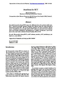
3.1 The diagram of MH prediction and residual reconstruction as post-processing for hyperspectral image reconstruction. . . . . . . . . . . . . . . . . . . . . .
vi
33
3.2 (a) Generation of multiple hypotheses from a search window with window size ω. (Red indicates the current pixel-vector of interest, and green indicates a possible hypothesis pixel-vector.) (b) Generation of hypotheses via nonuniform or uniform spectral-band partitioning and zero padding. . . . . . . .
34
3.3 191 × 191 matrix of cross-band correlation coefficients of the Washington DC Mall HYDICE dataset. White = ± 1. Black = 0. S1 , S2 , S3 and S4 are the four segments of spectral-band partitioning based on correlation coefficients. .
35
3.4 Formation of a prediction using multiple hypotheses and the corresponding weights. hSi (i = 1, 2, 3 and 4) is the hypothesis set generated using the ith segment of the hypotheses with zero padding. whSi are the corresponding set of weights for hypothesis set hSi . . . . . . . . . . . . . . . . . . . . . . . . .
36
3.5 The mean distance vector for all pixel-vectors in the CPPCA-reconstructed Washington DC Mall dataset at K/N = 0.2. Search window size ω = 3. Four segments in spectral-band partitioning are used for hypothesis generation. . .
41
3.6 False color images: (a) Washington DC Mall, using bands 30, 40 and 50 for red, green and blue, respectively. (b) Indian Pines, using bands 10, 20 and 30 for red, green and blue, respectively. (c) University of Pavia, using bands 20, 40 and 60 for red, green and blue, respectively. (d) Low Altitude, using bands 40, 50 and 60 for red, green and blue, respectively. . . . . . . . . . . . . . . .
41
3.7 The average SNR of the reconstructed (a) Indian Pines (b) Washington DC Mall (c) University of Pavia at sampling subrate K/N = 0.2 with various search window sizes for hypothesis generation. . . . . . . . . . . . . . . . . vii
42
3.8 Classification accuracy (%) using (a) FLDA-MLE (b) SVM for the reconstructed Indian Pines dataset with various algorithms. . . . . . . . . . . . . .
46
3.9 Classification accuracy (%) using (a) FLDA-MLE (b) SVM for the reconstructed University of Pavia dataset with various algorithms. . . . . . . . . .
47
3.10 For the AVIRIS Indian Pine dataset: (a) Ground truth map and (j) Class label. Classification maps obtained by MLE on (b) Original dataset, OA = 76.19%, and the reconstructed dataset using: (c) CPPCA, OA = 62.85%, (d) C-CPPCA, OA = 49.37%, (e) MH(NU)-CPPCA, OA = 97.63%, (f) MH(U)-CPPCA, OA = 98.35%, (g) MH(NU)-C-CPPCA, OA = 97.69%, (h) MH(U)-C-CPPCA, OA = 97.18%, and (i) MT-BCS, OA = 65.51%. . . . . . . . . . . . . . . . . . . .
48
3.11 For the AVIRIS Indian Pine dataset: (a) Ground truth map and (j) Class label. Classification maps obtained by SVM on (b) Original dataset, OA = 86.36%, and the reconstructed dataset using: (c) CPPCA, OA = 70.43%, (d) C-CPPCA, OA = 74.85%, (e) MH(NU)-CPPCA, OA = 87.44%, (f) MH(U)-CPPCA, OA = 89.89%, (g) MH(NU)-C-CPPCA, OA = 88.23%, (h) MH(U)-C-CPPCA, OA = 86.90%, and (i) MT-BCS, OA = 69.91%. . . . . . . . . . . . . . . . . . . .
49
3.12 For the ROSIS University of Pavia dataset: (a) Ground truth map and (j) Class label. Classification maps obtained by MLE on (b) Original dataset, OA = 88.22%, and the reconstructed dataset using: (c) CPPCA, OA = 79.97%, (d) C-CPPCA, OA = 71.96%, (e) MH(NU)-CPPCA, OA = 96.22%, (f) MH(U)CPPCA, OA = 95.58%, (g) MH(NU)-C-CPPCA, OA = 97.83%, (h) MH(U)C-CPPCA, OA = 97.54%, and (i) MT-BCS, OA = 83.53%. . . . . . . . . . . viii
50
3.13 For the ROSIS University of Pavia dataset: (a) Ground truth map and (j) Class label. Classification maps obtained by SVM on (b) Original dataset, OA = 94.62%, and the reconstructed dataset using: (c) CPPCA, OA = 82.63%, (d) C-CPPCA, OA = 83.48%, (e) MH(NU)-CPPCA, OA = 97.59%, (f) MH(U)CPPCA, OA = 97.13%, (g) MH(NU)-C-CPPCA, OA = 97.85%, (h) MH(U)C-CPPCA, OA = 97.73%, and (i) MT-BCS, OA = 88.94%. . . . . . . . . . .
51
4.1 Hypothesis generation within a search window. . . . . . . . . . . . . . . . .
59
4.2 (a) The LR input image. (b) Results of the Lenna image magnified by a factor of s = 2. Top-row (left to right): the original HR image, bicubic interpolation (RMSE: 7.0); bottom-row (left to right): Yang’s method [54] (RMSE: 5.39), our method (RMSE: 5.82). . . . . . . . . . . . . . . . . . . . . . . . . . . .
60
4.3 Results of the Lenna image magnified by a factor of s = 4. Top-row (left to right): the original HR image, bicubic interpolation (RMSE: 9.21); bottomrow (left to right): Yang’s method [54] (RMSE: 7.81), our method (RMSE: 8.18). . . . . . . . . . . . . . . . . . . . . . . . . . . . . . . . . . . . . . .
ix
61
CHAPTER 1 INTRODUCTION
1.1 Overview Compressed sensing (CS) [5, 7, 15, 8] is a recently developed mathematical paradigm that, under certain conditions, exactly recovers signals sampled at sub-Nyquist rates via a linear projection onto a random basis. The CS of images faces several challenges including a large computational cost associated with multidimensional signal reconstruction and a huge memory burden when the random sampling operator is represented as a dense matrix. To address these issues, structurally random matrices (SRMs)(e.g., [14]) can be used to provide a sampling process with little computation and memory. An alternative to SRMs is to limit CS sampling to relatively small blocks (e.g., [27, 40]). Block-based CS (BCS) with smoothed projected Landweber reconstruction (BCS-SPL) [40], as well as a multiscale variant (MS-BCS-SPL) [23] deployed in the domain of a discrete wavelet transform (DWT), typically provides much faster reconstruction than techniques based on full-image CS sampling. In video CS, a motion-compensated reconstruction (MC-BCSSPL) [41] extends this advantage to the CS reconstruction of video in which one or more frames are used to make predictions of the current frame such that the resulting residual is more efficiently reconstructed.
1
In this thesis, we extend this concept of prediction plus residual reconstruction to the use of multihypothesis (MH) prediction (e.g., [45]). That is, we couple BCS-SPL with MH prediction for still-image reconstruction. We first reconstruct the image with an initial BCS-SPL reconstruction, cull predictions for each image block from spatially surrounding blocks, and then finally reconstruct the resulting prediction-residual image. We also consider a similar multiscale variant in which the MH prediction occurs in the wavelet domain. In all cases, we determine the MH prediction in the domain of CS random projections. Due to the ill-posed nature of the resulting prediction problem, we apply Tikhonov regularization [47] to arrive at a solution. Experimental results indicate a significant gain in PSNR as compared to the original BCS-SPL as well as to a popular still-image reconstruction based on total-variation (TV) minimization [6]. We also apply this basic framework of MH prediction and residual reconstruction to recover hyperspectral imagery from random projections. For this data too, we find that techniques employing MH prediction significantly outperform alternative strategies that do not use MH prediction. We also explore the use of MH prediction with image super-resolution (SR), an active area of current research offering solutions to overcome the resolution limitations of the low-cost digital imaging systems as well as imperfect imaging environments. A popular SR paradigm consists of synthesizing a new high-resolution (HR) image by using one or more low-resolution (LR) images [42]. In contrast, in this thesis, we focus on SR image reconstruction given only a single LR image. In our proposed framework, each patch of the LR image is represented as a linear combination of spatially surrounding patches which are consider to be multiple hypotheses for the current patch. The coefficients of 2
the resulting linear combination are calculated using Tikhonov regularization and then are used to generate the HR image.
1.2 Contributions In this thesis, we present three key contributions for CS reconstruction and SR for images: • We propose an algorithm for the CS reconstruction of a single still image that exploits the high degree of spatial correlation in images by incorporating MH prediction to enhance CS reconstruction, using a distance-weighted Tikhonov regularization to find the best linear combination of hypotheses. The resulting prediction is used to create a measurement-domain residual of the signal to be recovered—such a residual is typically more compressible than the original making it more amenable to CS reconstruction. This contribution was initially published as [12]. • We extend the MH-prediction plus residual-reconstruction framework to incorporate it into the reconstruction of hyperspectral data from random projections. This contribution is the subject of an upcoming publication [11]. • Finally, we further extend the MH-prediction paradigm for single-image SR, exploiting self-similarities existing between image patches within a single image. The fact that no high-resolution (HR) training set is required for SR based on this MH prediction makes it more practical than a competing SR based on sparse representation since there is no guarantee that a relevant HR training set is available for low-resolution input images in all situations. This contribution is the subject of an upcoming publication [10]. The remainder of this thesis is organized as follows. Chap. 2 discusses in detail our proposed MH prediction for still-image reconstruction and provides experimental results comparing it to other CS reconstruction schemes. Chap. 3 describes the procedure of using MH prediction to enhance hyperspectral data reconstruction from random projections as well as the details concerning the generation of the multiple hypotheses. Chap. 4 presents our MH prediction framework for single-image SR and compares it with other SR algorithms. Finally, Chap. 5 makes some concluding remarks. 3
CHAPTER 2 COMPRESSED-SENSING RECOVERY OF IMAGES WITH MULTIHYPOTHESIS PREDICTION
In this chapter, we describe the general process of multihypothesis (MH) prediction as it relates to the compressed-sensing (CS) reconstruction a single 2D image. We first briefly review background theory of CS for images (Sec. 2.1) before presenting the specifics of MH prediction with Tikhonov regularization (Sec. 2.2). We conclude this chapter with the presentation of a battery of experimental results (Sec. 2.3). We note that the material in this chapter has previously been published as [12].
2.1 Background Suppose we want to recover real-valued signal x ∈ RN from M measurements such that M ≪ N; i.e., y = Φx, where y ∈ RM , and Φ is an M × N measurement matrix with subsampling rate, or subrate, being S = M/N. CS theory holds that, if x is sufficiently sparse in some transform basis Ψ, then x is recoverable from y by the optimization, xˆ = argmin kΨxk1 ,
such that y = Φx,
(2.1)
x∈RN
as long as Φ and Ψ are sufficiently incoherent, and M is sufficiently large. High-dimensional signals, such as images or video, impose a huge memory burden when explicitly storing the sampling operator Φ as a dense matrix. In addition, the reconstruction process will be 4
time consuming if the dimensionality is large. To assuage the computation complexity, in [27, 40], an image is partitioned into B × B non-overlapping blocks while sampling is applied on a block-by-block basis. In such BCS, the global measurement matrix takes a block-diagonal structure,
ΦB 0 · · · 0 0 Φ ··· 0 B , Φ= . .. .. .. . . 0 · · · 0 ΦB
(2.2)
wherein ΦB independently samples blocks within the image. That is, yi = ΦB xi , where xi is a column vector with length B 2 representing block i of the image, and ΦB is a MB × B 2 measurement matrix such that the subrate of BCS is S = MB /B 2 . In [27, 40], reconstruction uses a procedure that couples projected Landweber (PL) iteration with a smoothing operation intended to reducing blocking artifacts. The overall technique was called BCS-SPL in [40]. BCS-based techniques such as BCS-SPL that rely on a block-based sampling operator can be at a disadvantage in terms of reconstruction quality since CS sampling generally works better the more global it is. To improve reconstruction quality, in [23], BCS-SPL was deployed independently within each subband of each decomposition level of a wavelet transform of an image to provide multiscale sampling and reconstruction; the resulting algorithm for image reconstruction was called MS-BCS-SPL. Motion estimation (ME) and motion compensation (MC) are widely used and crucial components to traditional video-coding system. In [41], this ME/MC framework was 5
incorporated into the reconstruction process of BCS-SPL for video. The resulting motioncompensated version of BCS-SPL was called MC-BCS-SPL. In this approach, a motioncompensated prediction of the current frame is created during reconstruction such that some CS image-reconstruction algorithm is applied to the residual between the current frame and its ME/MC prediction. Specifically, if a ME/MC prediction is similar to the original frame, then the prediction residual will be more amenable to CS reconstruction since the residual is typically more compressible than the original frame itself. Suppose x˜ is a prediction of original frame x which satisfies x˜ ≈ x; the residual between the two signals is r = x − x˜. With a measurement basis Φ, the projection of r is q = Φr = y − Φ˜ x. The final reconstruction of y is calculated as xˆ = x˜ + Reconstruct(q, Φ), where Reconstruct(·) is some suitable CS image reconstruction. To produce a highly compressible residual, one should create a prediction that is as close as possible to x, which implies that the following optimization problem is desired, x˜ = argmin kx − pk22 ,
(2.3)
p∈P(xref )
where P(xref ) is the set of all ME/MC predictions that can be made from a reference frame, xref . However, since x is unknown in CS reconstruction, solving (2.3) directly is infeasible. Instead, one approach is to reformulate (2.3) as x˜ = argmin kˆ x − pk22 ,
(2.4)
p∈P(xref )
wherein some initial reconstruction, xˆ, is used as a proxy for x in (2.3); this is, in fact, the approach taken in [41, 34]. 6
An alternative is to recast the optimization of (2.3) from the ambient signal domain of x into the measurement domain of y; specifically, x˜ = argmin ky − Φpk22 .
(2.5)
p∈P(xref )
The Johnson-Lindenstrauss (JL) lemma [33] holds that L points in RN can be projected into a K-dimensional subspace while approximately maintaining pairwise distances as long as K is sufficiently large with respect to L. Specifically, for ǫ > 0 and every set Q of L points in RN , there exists mapping f : RN → RK such that, for all x1 , x2 ∈ Q, (1 − ǫ) kx1 − x2 k22 ≤ kf (x1 ) − f (x2 )k ≤ (1 + ǫ) kx1 − x2 k22 ,
(2.6)
as long as K ≥ O(ǫ−2 log L). This suggests that the solution of (2.5) will likely coincide with that of (2.3). The next section explores a general strategy for implementing (2.5) with MH prediction and incorporates it to still-image CS reconstruction.
2.2 Multihypothesis Prediction with Tikhonov Regularization For a MH CS reconstruction of still-image, the goal is to reformulate (2.5) so that, instead of choosing a single prediction, or hypothesis, we find an optimal linear combination of all hypotheses contained in some search set; i.e, (2.5) becomes x˜i = Hi wˆi where wˆi = argmin kyi − ΦB Hi wk22 ,
(2.7)
w
and we have also recast (2.5) for block-based prediction with i being the block index. Here, Hi is a matrix of dimensionality B 2 × K whose columns are the rasterizations of the possible blocks within the search space of the reference image. In this context, w ˆi is a column vector which represents a linear combination of the columns of Hi . However, because 7
usually M 6= K, the ill-posed nature of the problem requires some kind of regularization in order to differentiate among the infinite number of possible linear combinations which lie in the solution space of (2.7). The most common approach to regularizing a least-squares problem is Tikhonov regularization [47] which imposes an ℓ2 penalty on the norm of wˆi , wˆi = argmin kyi − ΦB Hi wk22 + λ kΓwk22 ,
(2.8)
w
where Γ is known as the Tikhonov matrix and λ is the regularization parameter; this strategy for MH prediction was initially proposed in [48]. The Γ term allows the imposition of prior knowledge on the solution—we take the approach in [48] that hypotheses which are the most dissimilar from the target block should be given less weight than hypotheses which are most similar. Specifically, a diagonal Γ takes the form of
0 kyi − ΦB h1 k2 . , .. Γ= 0 kyi − ΦB hK k2
(2.9)
where hj are the columns of Hi , j = 1, . . . , K. For each block then, w ˆi can be calculated directly by the closed form solution, � �−1 wˆi = (ΦB Hi )T (ΦB Hi ) + λ2 ΓT Γ (ΦB Hi )T yi .
(2.10)
2.2.1 MH-BCS-SPL Above, we considered applying MH prediction for the CS of a still image. To generate hypotheses for each block within an image, the matrix of hypotheses, Hi , is assembled 8
from an initial reconstruction, x¯, of the image x using either BCS-SPL or MS-BCS-SPL. That is, for each block in x¯, multiple predictions are generated from its spatially surrounding blocks in the initial reconstruction. Specifically, suppose image x is split into blocks of size B × B in BCS; each block is further divided into subblocks of size b × b. Predictions are created for each individual subblock of the block by sliding a b × b mask across the entire search window to create all candidate predictions for each subblock. Since the block size is B × B, the region in the block outside of the b × b subblock is set to all zeros; the resulting B × B “zero-padded” block is then placed as a column in Hi ; Hi thus contains all the predictions for all of the subblocks of block i. This subblock-based MH-prediction process is illustrated in Fig. 2.1(a)–(c). The parameter λ in (2.8) controls the regularization. Unfortunately, there does not appear to be a straightforward approach for finding an optimal value without foreknowledge of x. Some possible approaches to choose an appropriate λ include the L-curve [30], generalized cross validation (GCV), and the discrepancy principle. Through empirical analysis, we test a set of λ values and choose the one gives the best performance. We incorporate the proposed MH-based prediction into BCS-SPL image reconstruction, resulting in a technique we call MH-BCS-SPL (see Algorithm 1). In MH-BCS-SPL, MH prediction and residual reconstruction are repeated with increasing subblock size in order to improve the quality of the recovered image. The original BCS-SPL reconstruction of [40] uses a block size of B = 32 and a dualtree DWT (DDWT) [35] as the sparsity transform Ψ. In MH-BCS-SPL, we start with an initial subblock size of b = 16 and an initial search window of w = 8. The subblock 9
size b and search window w are increased based on a criterion involving structural similarity (SSIM) [51]. As a stopping criterion, we apply cross validation [52] to predict the performance. Specifically, three measurements as a holdout set yH are used for the performance test. For example, at subrate = 0.1 and block size B = 32, the measurement matrix Φ ∈ R102×1024 has three more rows than ΦR ∈ R99×1024 which is used for reconstruction. ΦH ∈ R3×1024 is the measurement matrix for the holdout set. In other words, ΦB = [ΦR ; ΦH ] and y = [yR ; yH ]. The residual calculated in the projected domain is R = kΦH x − ΦH xˆk2 = kyH − ΦH xˆk2 .
(2.11)
This means that, if xˆ is close to x, then R should be small.
Algorithm 1 MH-BCS-SPL Input: y = [yR ; yH ], ΦB = [ΦR ; ΦH ], Ψ, x¯ (initial BCS-SPL reconstruction), b (initial subblock size), w (initial search window size), B = 32 (block size), τ . Output: x¯. Initialization: i = 1, x ˆ0 = x ¯, s0 = 0, R0 = +∞. repeat x, yR , ΦR , b, w, B) x ˜i = MH Prediction(¯ x ˆi = x ˜i + BCS-SPL(yR − ΦR x ˜i , ΦR , Ψ, B) Compute si = SSIM(ˆ xi , x ˆi−1 ), Ri = ||yH − ΦH xˆi ||2 if b < B then if (Ri < Ri−1 & |si − si−1 | ≤ τ ) or Ri > Ri−1 then b ← b × 2, w ← w × 2 end if end if Update x ¯ ← xˆi i=i+1 until Ri > Ri−1 & b = B
10
2.2.2 MH-MS-BCS-SPL As described in [23], MS-BCS-SPL performs both CS measurement and reconstruction in the wavelet domain; i.e., the CS measurement process becomes y = ΦΩx, where Ω is a 3-level DWT with the popular 9/7 biorthogonal wavelet. Block size depends on transform level, with Bl = 16, 32, and 64 for levels l = 1, 2, and 3, respectively (l = 3 is the highest-resolution level). A DDWT is again used as the sparsity transform Ψ. We now formulate a MH version of MS-BCS-SPL by performing MH prediction within the wavelet domain. That is, in MH-MS-BCS-SPL, multiple predictions for a block are made using the procedure of Fig. 2.1(a) applied in the wavelet domain of the MS-BCSSPL reconstructed image. In the case that the subblocks are smaller than the block size (i.e., bl < Bl ), the MH prediction is carried out within a subband of a DWT. However, for the bl = Bl case, predictions are calculated using a redundant DWT (RDWT) for Ω. Such a RDWT is an overcomplete transform, effectively created by eliminating downsampling from the traditional DWT; see, e.g., [20]. In this latter case, the multiple hypotheses are culled from the various RDWT phases associated with the subband as illustrated in Fig. 2.1(d). In our experiments, λ = 0.035 is used when bl < Bl , and λ = 0.5 when bl = Bl . The initial subblock size bl is one eighth of the block size Bl at each decomposition level. The initial search window is set to w = 1. For the stopping criterion, we did not apply cross validation, as we found that the reduced number of measurements y due to the holdout set would adversely affect the recovery performance since CS sampling is deployed in the wavelet domain. In this case, a threshold τs calculated from the SSIM between two 11
successive residual reconstructed images is used as a stopping criterion: τs = 0.9995 when subrate = 0.1, 0.2, and 0.3; τs = 0.99995 when subrate = 0.4 and 0.5. Algorithm 2 details the MH-MS-BCS-SPL procedure.
Algorithm 2 MH-MS-BCS-SPL Input: y, Φ, Ψ, x ¯, L = 3 (wavelet transform level), {bl }, w, {Bl }, τs . Output: x¯. Initialization: i = 1, x ˆ0 = x ¯, s0 = 0. repeat if bl = Bl for each level l then x˙ i = ΩRDWT x ¯ {Perform redundant wavelet transform} else x˙ i = ΩDWT x ¯ {Perform discrete wavelet transform} end if for 1 ≤ l ≤ L do for each subband θ ∈ {H, V, D} do ˜˙i (θ) = MH Prediction(x˙ i (θ), y(θ), Φ, Bl , bl , w) x end for end for ˜˙i x ˜i = Ω−1 x x ˆi = x ˜i + BCS-SPL(y − Φ˜ xi , Φ, Ψ, {Bl }) Compute si = SSIM(ˆ xi , x ˆi−1 ) if |si − si−1 | ≤ τ and bl < Bl for each level l then for 1 ≤ l ≤ L do bl ← bl × 2 end for w ←w×2 end if Update x ¯ ← xˆi until |si − si−1 | ≤ τs
2.3 Experimental Results The performance of the MH-BCS-SPL and MH-MS-BCS-SPL is evaluated on a number of grayscale images of size 512×512 (see Fig. 2.2) with τ = 0.0001. We compare to the original BCS-SPL [40] and MS-BCS-SPL [23] as well as to the TV reconstruction described in [6] and a multiscale variant of GPSR as described in [44]. Block-based sam12
pling operator ΦB is a B × B dense Gaussian matrix; on the other hand, TV uses the scrambled block-Hadamard SRM of [14] to provide a fast whole-image CS sampling. The multiscale GPSR (MS-GPSR) uses the same Ω as MS-BCS-SPL in implementing GPSR1 [18] reconstruction at each DWT level. We use our implementations2 of BCS-SPL and MS-BCS-SPL, and l1 -MAGIC3 for TV. The reconstruction performance of the various algorithms under consideration is presented in Table 2.1 and Table 2.2. In all cases except the “Barbara” and “Barbara2” images, MH-MS-BCS-SPL performs uniformly better than other algorithms. For “Barbara,” MHBCS-SPL provides a substantial gain in reconstruction quality over TV, generally on order of a 5- to 7-dB increase in PSNR. A visual comparison of the various algorithms is shown in Fig. 2.3. As can be seen in Table 4.2, in terms of execution time, reconstruction with MH-BCSSPL and MH-MS-BCS-SPL is, as expected, slower than BCS-SPL and MS-BCS-SPL due to iterated MH prediction. Both algorithms run for less than 3 minutes on a quadcore 2.67GHz machine. On the other hand, the execution times of TV are much slower than MHBCS-SPL and MH-MS-BCS-SPL, with TV requiring more than 20 minutes to reconstruct a single image even with fast SRM implementation of the sampling operator.
1
http://www.lx.it.pt/˜mtf/GPSR/
2
http://www.ece.msstate.edu/˜fowler/BCSSPL/
3
http://www.l1magic.org
13
(c)
(a)
S1 S2
S1
0
0
S2
0
0
0
0
S3 S4
0
0
0
0
S3
0
0
S4
zero-padding current subblock hypothesis subblock search window
(d)
Multi-phase RDWT
(b)
S2
S3
S4 B
b
S1
even-even phase
even-odd phase
odd-even phase
odd-odd phase
Figure 2.1 (a) Generation of multiple hypotheses for a subblock in a search window; (b) generation of multiple hypotheses for each b × b subblock within a B × B block; (c) zero-padding of subblock predictions into blocks; (d) generation of multiple hypotheses within the multiple phases of an RDWT (four phases are shown—each phase has the same size as the corresponding DWT subband and results from various combinations of even and odd downsampling in the horizontal and vertical directions).
14
Figure 2.2 The 512 × 512 grayscale still images used in the experiments. Top row (left to right): Lenna, Barbara, Barbara2, Goldhill; Middle row (left to right): Mandrill, Peppers, Boat, Cameraman; Bottom row (left to right): Clown, Crowd, Couple, Girl.
15
Table 2.1 Image Reconstruction PSNR (dB), part I 0.1
Original MH MS MH-MS MS-GPSR TV
27.93 29.85 31.48 31.61 30.30 29.84
Original MH MS MH-MS MS-GPSR TV
22.28 27.89 23.84 24.28 24.03 22.95
Original MH MS MH-MS MS-GPSR TV
23.64 26.83 25.14 25.61 25.28 323.90
Original MH MS MH-MS MS-GPSR TV
26.57 27.67 28.97 29.07 28.39 27.52
Original MH MS MH-MS MS-GPSR TV
20.45 20.47 21.45 21.66 21.52 20.53
Original MH MS MH-MS MS-GPSR TV
28.83 30.28 31.75 32.08 29.25 30.36
BCS-SPL
BCS-SPL
BCS-SPL
BCS-SPL
BCS-SPL
BCS-SPL
Algorithm
Subrate 0.2 0.3 Lenna 31.27 33.41 32.85 34.73 34.59 36.61 34.88 36.79 33.60 35.29 32.93 35.05 Barbara 23.78 25.32 31.46 33.63 25.12 26.05 26.42 27.98 25.24 26.06 24.48 26.30 Barbara2 25.56 27.19 30.19 32.03 27.31 29.12 28.87 31.06 27.34 28.82 26.24 28.51 Goldhill 28.92 30.42 30.28 31.82 31.06 32.75 31.35 33.06 30.55 32.10 29.87 31.63 Mandrill 21.80 22.90 22.36 24.03 23.07 24.69 23.20 24.82 22.92 24.27 22.02 23.44 Peppers 31.98 33.72 32.82 34.32 34.59 35.76 34.73 35.96 31.90 33.03 33.14 34.70
16
0.4
0.5
35.15 36.34 37.82 38.32 36.29 36.82
36.71 37.82 38.94 39.74 37.73 38.43
26.88 35.68 27.27 32.95 27.50 28.42
28.51 37.29 28.83 36.21 29.64 30.78
28.75 33.71 30.34 33.74 30.19 30.74
30.38 35.27 31.66 36.30 32.21 32.97
31.72 33.26 33.67 34.55 32.89 33.23
33.03 34.62 34.64 36.10 34.20 34.81
23.96 25.36 25.54 25.81 25.07 24.94
25.10 26.67 26.46 27.10 26.21 26.52
35.12 35.63 36.77 37.15 34.22 35.91
36.36 36.87 37.67 38.37 35.75 37.05
Table 2.2 Image Reconstruction PSNR (dB), part II Algorithm BCS-SPL
Original MH MS MH-MS MS-GPSR TV
BCS-SPL
Original MH MS MH-MS MS-GPSR TV
BCS-SPL
Original MH MS MH-MS MS-GPSR TV
BCS-SPL
Original MH MS MH-MS MS-GPSR TV
BCS-SPL
Original MH MS MH-MS MS-GPSR TV
BCS-SPL
Original MH MS MH-MS MS-GPSR TV
Subrate 0.2 0.3 Boat 25.14 27.78 29.57 26.17 29.30 31.18 27.35 30.08 31.98 27.46 30.38 32.23 26.52 29.21 30.84 26.42 29.24 31.28 Cameraman 26.02 30.36 33.65 29.86 33.97 36.57 31.05 36.54 39.98 31.71 38.08 42.85 29.53 34.76 39.59 30.87 35.08 38.32 Clown 24.46 29.65 31.87 28.78 32.80 35.02 29.06 32.72 35.65 29.48 33.89 36.20 27.93 31.58 33.95 27.94 31.18 33.48 Crowd 24.49 28.87 31.16 26.62 30.11 32.35 29.15 32.72 35.71 29.20 32.76 35.78 27.99 31.20 34.13 26.81 30.45 33.26 Couple 24.78 27.01 28.65 25.82 28.85 30.67 26.87 29.51 31.47 27.04 30.05 31.79 26.28 28.82 30.60 25.73 28.48 30.64 Girl 29.63 32.69 34.76 31.74 34.84 36.68 33.49 36.29 38.87 33.58 36.75 39.08 32.18 35.24 37.70 30.26 33.53 35.87 0.1
17
0.4
0.5
31.12 32.89 33.12 33.89 32.06 32.97
32.60 34.45 34.22 35.46 33.64 34.53
36.42 39.28 42.91 45.63 41.82 41.09
38.90 41.48 44.91 48.15 45.08 43.73
33.70 36.83 36.94 38.16 35.00 35.41
35.37 38.40 38.02 39.76 36.56 37.24
33.11 34.38 37.03 37.57 35.14 35.81
34.98 36.22 38.32 39.33 36.96 38.32
30.14 32.21 32.55 33.83 31.61 32.61
31.60 33.76 33.65 35.57 33.15 34.51
36.46 38.41 39.70 40.43 38.59 37.77
38.07 39.85 40.63 41.81 39.89 39.51
Figure 2.3 Reconstructed Barbara image for subrate = 0.1. Left-column (top to bottom): TV (22.95 dB), BCS-SPL (22.41 dB), MS-BCS-SPL (23.91 dB); right-column (top to bottom): MS-GPSR (24.05 dB), MH-BCS-SPL (27.92 dB), MH-MS-BCS-SPL (24.33 dB).
18
Table 2.3 Reconstruction time for Lenna at subrate = 0.3 Algorithm BCS-SPL MH-BCS-SPL MS-BCS-SPL MH-MS-BCS-SPL MS-GPSR TV
19
Time (sec.) 14.38 146.77 12.93 45.98 138.40 1211.96
CHAPTER 3 RECONSTRUCTION OF HYPERSPECTRAL IMAGERY USING MULTIHYPOTHESIS PREDICTION
Hyperspectral imagery (HSI) captures a dense spectral sampling of reflectance values over a wide range of the spectrum. This is often a double-edged sword—the availability of rich spectral information is expected to improve the performance of image-analysis techniques; however, this can come at the cost of increased computational complexity, over-dimensionality, and statistical ill-conditioning. Further, high-dimensional HSI data also increases communication costs associated the transmission of data from the remote sensor. As a consequence, some form of spectral dimensionality reduction is almost always required before HSI can be used in image-analysis applications; if this can be accomplished prior to downlink of the dataset from the remote sensor, communication costs can be significantly alleviated. There has been interest in using random projections effectuated directly within the hardware of the hyperspectral sensor to simultaneously reduce dimensionality as the HSI dataset is sensed, and sensor architectures for such random-projection-based spectral imaging have been proposed (e.g., [28]). In such a paradigm, the computational cost of dimensionality reduction is shifted from the resource-constrained remote-sensing platform to the more-capable ground-based receiver which is then burdened with the task of re20
construction of the HSI dataset from the random projections. There has been, of course, significant recent interest using CS to provide such reconstruction. Alternatively, Fowler [21] proposed a novel image reconstruction strategy—compressive-projection principal component analysis (CPPCA)—which recovers a hyperspectral dataset from spectral random projections using principal component analysis (PCA). CPPCA recovers not only the coefficients associated with the PCA transform, but also an approximation to the PCA transform basis itself [21]. The remainder of this chapter is organized as follows. In Sec. 3.1, several techniques— including those based on CS and CPPCA—for the reconstruction from random projections of hyperspectral data are reviewed. Then, in Sec. 3.2, we employ the general strategy of multihypothesis (MH) prediction developed in Chap. 2 for still images to the problem of HSI reconstruction, focusing as well on generation of hypotheses for HSI data. Finally, in Sec. 3.3, experimental results with various algorithms are presented. We note that the material in this chapter will constitute an upcoming publication [11].
3.1 Reconstruction From Random Projections Consider a dataset of M vectors X = [x1 · · · xM ], where each xm ∈ RN . We assume the signal-acquisition device applies N × K orthonormal random projection P to e = [e eM ] where each y em = PT xm has dimension K obtain random projections Y y1 · · · y
(K ≪ N); K/N is referred to as the subrate hereafter. To reconstruct an approximation b from the projections Y, e we could apply one of the several existing algorithms; we X overview three below, specifically, multi-task Bayesian compressive sensing (MT-BCS) 21
[32] in Sec. 3.1.1, CPPCA [21] in Sec. 3.1.2 and the recent proposed class-dependent CPPCA (C-CPPCA) [38] in Sec. 3.1.3.
3.1.1 MT-BCS CS (e.g., [5, 7, 15, 8]), in brief, produces a sparse signal representation directly from a small number of projections onto another basis, recovering the sparse transform coefficients via nonlinear reconstruction. The main tenet of CS theory holds that, if signal x ∈ RN can be sparsely represented (i.e., using only L nonzero coefficients) with some e = PT x under certain conbasis, then we can recover x from K-dimensional projections y
ditions. For recovery of a set of multiple, possibly correlated vectors X = [x1 · · · xM ],
there have been proposals for multi-vector extensions of CS under the name of “multitask” [32] CS; these, in turn, link closely to a larger body of literature on “simultaneous sparse approximation” (e.g., [19, 39, 53, 50, 49]). Below, we focus on MT-BCS [32] which introduces a hierarchical Bayesian framework into the multi-vector CS-recovery problem to share prior information across the multiple vectors.
3.1.2 CPPCA CPPCA [21] is driven by projections at the sensor onto lower-dimensional subspaces chosen at random. The CPPCA receiver, given only these random projections, recovers not only the coefficients associated with the PCA transform, but also an approximation to the PCA transform basis itself.
22
CPPCA reconstruction of a set of randomly projected vectors first entails an eigenvectorreconstruction process based on an approximation that uses Ritz vectors [43] as close representations of orthonormal projections of eigenvectors. Specifically, the PCA transform ˇ m = UT xm , where N × N transform matrix U of xm in dataset X = [x1 · · · xM ] is x emanates from the eigendecomposition of ΣX ; i.e., ΣX = UΛUT ,
(3.1)
where U contains the N unit eigenvectors of ΣX column-wise. CPPCA reconstruction e e = PT ΣX P) to obtain uses the first L Ritz vectors (essentially the eigenvectors of Σ Y
approximations of the first L principal eigenvectors in U corresponding to the L largest
eigenvalues in Λ. These approximate eigenvectors are then assembled into N × L matrix Ψ. The reconstruction of the dataset X is then produced in a pseudoinverse-based recovery of the PCA coefficients, b = Ψ(PT Ψ)⊤ Y, e X
(3.2)
The number of eigenvectors to recover is determined by the heuristic L = round(S/ log N) as proposed in [37]. The reader is referred to [21] for greater detail.
3.1.3 C-CPPCA C-CPPCA [38] can be viewed as an extension of original CPPCA reconstruction algorithm that incorporates classification into the reconstruction. For this approach, the sender-side sensing procedure is exactly the same as that employed in original CPPCA. e are firstly classified into one of several groups At the receiver, the random projections Y
using a pixel-wise classification, such as a support vector machine (SVM) [3]. After the 23
grouping procedure, the CPPCA reconstruction algorithm is employed for each class independently. More specifically, a small set of “exemplars” is chosen randomly from the projections e these exemplars are recovered using MT-BCS (which is efficient at recovering a small Y;
number of samples, unlike CPPCA which requires more samples to be effective). These reconstructed samples are then clustered into different groups, producing a “pseudo” a
priori label information (training data). A trained pixel-wise classifier is then employed e into one of K0 classes. Thus, each Y e is further partito classify each pixel in each Y
e k , k = 1, . . . , K0 , based on this classification. Finally, traditional tioned into K0 groups, Y
CPPCA reconstruction is employed individually on each class.
It has shown in [38] that the C-CPPCA strategy outperforms original CPPCA. This can be attributed to multiple modes in the data distribution arising from the presence of multiple classes/objects in the image. Hence, the C-CPPCA method employs statistics pertinent to each class as opposed to the average statistics over all classes. The resulting reconstruction then exploits individual local geometrical distributions as provided by the covariance matrix of each class as opposed to a single aggregated distribution as is employed in original CPPCA. A detailed discussion for C-CPPCA can be found in [38].
3.2 Reconstruction Using Multihypothesis Prediction With the success of applying MH prediction to CS natural images reconstruction as was demonstrated in Chap. 2, in this section, we incorporate the framework of MH prediction plus residual reconstruction into hyperspectral data reconstruction from random 24
¯ is a prediction which satisfies projections. Specifically, suppose that x is a vector and x ¯ ≈ x. The residual is r = x − x ¯ . With a N × K orthonormal random projection P, the x e − PT x ¯ . The final reconstruction of y e is calculated as projection of r is q = PT r = y
b=x ¯ + Reconstruct(q, P), where Reconstruct(·) is some suitable signal reconstruction x (e.g., CS or CPPCA).
As stated in Sec. 2.1, to create a prediction that is as close as possible to x, the following optimization problem is desired, ¯ = argmin kx − zk22 , x
(3.3)
z∈P(Xref )
where P(Xref ) is the set of predictions that can be made from some reference dataset, Xref . However, since x is unknown in CS or CPPCA reconstruction, an alternative is to recast the optimization of (3.3) from the ambient signal domain of x into the measurement e as in (2.5); specifically, domain of y
2 ¯ = argmin y e − PT z 2 . x
(3.4)
z∈P(Xref )
Instead of choosing a single prediction, or hypothesis to reformulate (3.4), we aim to find an optimal linear combination of all hypotheses contained in the reference set P(Xref ); ¯ = Hw b where i.e., (3.4) becomes x
2 e − PT Hw 2 . b = argmin y w
(3.5)
w
Here, H is a matrix of dimensionality N ×KH whose columns are KH possible hypotheses b is a column vector which represents a linear combination of the columns in P(Xref ), and w 25
of H. To regularize the ill-posed nature of (3.5) (necessary since usually K 6= KH ), Tikhonov regularization [47] is used,
2
e − PT Hw 2 + λ kΓwk22 , b = argmin y w
(3.6)
w
where Γ is a diagonal matrix has the same structure as in (2.9), i.e.,
T e − P h1 2 0 y . , .. Γ=
y e − PT hK 0 H
(3.7)
2
b can be where h1 , h2 , . . . , hKH are the columns of H. For each pixel-vector, then, w calculated directly by the usual Tikhonov solution, b = w
�
PT H
�T
�−1 � �T e. P T H + λ2 ΓT Γ PT H y
(3.8)
For the reference dataset Xref , an initial reconstruction (i.e., using CS or CPPCA withb is used.1 Further more, once we have reconstructed the dataset via out MH prediction) X
MH prediction and residual reconstruction, we can use the current reconstruction as the reference dataset Xref for a subsequent MH prediction and residual reconstruction, further
improving the quality of the reconstructed data in an iterative fashion. A general diagram of this iterative post-processing algorithm is shown in Fig. 3.1.
3.2.1 Hypothesis Generation Hyperspectral data usually includes large number of homogeneous regions. For each sample, its neighboring pixel-vectors will likely share similar spectral characteristics. The 1
Alternatively, some other hyperspectral dataset(s) could be used as a dictionary for Xref depending on availability.
26
contextual information in hyperspectral data has already been taken into account for classification [46, 13]. To generate multiple hypotheses for one sample, all the neighboring pixel-vectors in a search window with size ω are considered. This hypothesis search procedure is illustrated in Fig. 3.2(a). All the hypotheses are then placed as columns of the hypothesis matrix H. Since the spectral bands of a hyperspectral image are correlated, they can be further partitioned into several groups based on the correlation coefficients between bands such that the bands in each group are highly correlated with one another [16]. For example, Fig. 3.3 shows the correlation coefficients between bands of the Washington DC Mall dataset. This spectral-band partitioning based on correlation coefficients is denoted as nonuniform (NU) partitioning. Another, simpler spectral-band partitioning is to partition the bands uniformly—i.e., each group has the same number of bands—this is denoted as uniform (U) partitioning. With either of the two partitioning methods, each hypothesis pixelvector can be divided into several segments. Assume a N-dimensional pixel-vector is divided into four segments using uniform partitioning, then four hypotheses can be created by keeping only one of the four segments and padding the other segments with zeros to form a N-dimensional vector. This hypothesis generation based on spectral-band partitioning is shown in Fig. 3.2(b). If KH hypotheses are drawn from the search window, and α segments are used for spectral-band partitioning, the total number of hypotheses in H is αKH . This hypothesis generation from the segmented spectral bands makes the weights calculated for the hypotheses adjustable to different segments. The details are shown in Fig. 3.4. One may 27
be interested in how can we obtain the correlation coefficients of the original dataset to perform spectral-band partitioning since we only have the reconstructed dataset at the reconstruction side. Usually, we assume that the correlation coefficients between the spectral bands are fixed and known a priori for a given hyperspectral sensor since all images taken by this sensor would have similar correlation coefficients. Other alternatives would be to estimate the correlation coefficients from the initial reconstructed dataset or simply use uniform band partitioning. Spectral-band partitioning based on correlation coefficients may not accurately capture the true correlation between bands since the dataset at hand is the reconstructed dataset, not the original. To analyze the accuracy of spectral-band partitioning based on correlation coefficients, we take the Washington DC Mall dataset as an example. According to the correlation coefficients map of the original dataset in Fig. 3.3, the spectral bands are partitioned into four segments with band indices 1–55, 56–102, 103–132, and 133–191. For each pixel-vector in the image, we generate its hypothesis matrix H following the procedures described in Fig. 3.2(a) and (b) with non-uniform partitioning, storing them in the order as shown in Fig. 3.4. For the mth pixel vector in the dataset, we can calculate the Euclidean norms between the projection of the original pixel vector and the projections of all hypothesis em , we devectors, which are the diagonal terms of Γ in (2.9). For projected vector y � �
T T fine a distance vector Dm = y em − P hαKH , where h1 , . . . , em − P h1 · · · y 2
2
em . In other words, the j th spectralhαKH are the αKH columns of the H matrix for y
band partition generates a set of KH hypotheses in H; this subset has a distance vector 28
�
T T Dm (j) = y e − P h(j−1)×KH +1 2 · · · y e − P hj×KH 2 , where h(j−1)×KH +1 , . . . , �
hj×KH are KH columns in H. As a consequence, each pixel vector is associated with a distance vector calculated using its corresponding projection and hypothesis matrix. For ¯ is calcua hyperspectral image with M pixel vectors, the global mean distance vector, D, lated as � M M � X X 1 1 ¯ = Dm = D M m=1 M m=1 Dm (1) · · · Dm (α)
�
�
¯ ¯ = D(1) , (3.9) · · · D(α) ¯ where D(j) is the mean calculated over the dataset for spectral-band partition j (j = ¯ for all pixel vectors in the initial 1, . . . , α). For example, the mean distance vector D CPPCA-reconstructed Washington DC Mall image is shown in Fig. 3.5 for α = 4 spectralband partitions. We argue that the last two spectral-band partitions depicted in Fig. 3.5 can be merged together since the distance between the original pixel vector and the hypothesis vector in the projection domain is very close for hypotheses formed with the third and fourth partitions, respectively. To make this merging decision automatically, we calculate the ¯ (scalar) mean of the D(j) vector as µj which we then normalize such that µj ∈ [0, 1]. Two consecutive partitions are merged together if |µj − µj+1 | ≤ σ, where σ is a threshold (we use σ = 0.1 in subsequent experiments). Consequently, we develop a two-phase spectral-band partitioning process. In the first phase, the spectral-band partitioning is based on the correlation coefficients; in the second phase, the corresponding partitions of the hypotheses which share similar distances in the 29
projection domain are merged together. The resulting spectral-band partitions for different hyperspectral images are tabulated in Table 3.1. On the other hand, for uniform partitioning, we simply choose four partitions for the first phase and two partitions for the second phase in order to compare with non-uniform partitioning. Table 3.1 Spectral-band partitions for non-uniform partitioning Dataset Washington DC Mall (307 × 307 × 191) University of Pavia (610 × 340 × 103) Low Altitude (512 × 512 × 224) Indian Pines (145 × 145 × 220)
1st phase 1-55, 56-102 103-132, 133-191 1-40, 41-68 69-76, 77-103 1-40, 41-112, 113-152 153-166, 167-224 1-37, 38-102, 103-150 151-162, 162-220
2nd phase 1-55, 56-102 103-191 1-68, 69-76 77-103 1-40, 41-112 113-224 1-37, 38-102 103-220
3.2.2 Stopping Criterion The aforementioned multihypothesis-prediction and residual-reconstruction procedures are iterated to achieve high quality reconstruction. As a criterion to stop these iterations, we apply cross validation [52] to predict performance. Specifically, the orthonormal random projection P = [PR , PH ], where P ∈ RN ×K , PR ∈ RN ×(K−L0 ) , PH ∈ RN ×L0 , and L0 ≪ K. For a hyperspectral image of M pixel-vectors X ∈ RN ×M , PR is used b R ∈ R(K−L0 )×M for reconstruction, and PH is used to to generate random projections Y
b H ∈ RL0 ×M as a holdout set for the performance test. In generate random projections Y
30
b = [Y b R; Y b H ]. The residual calculated in the projected domain using the other words, Y
holdout set is
b
T b b R = PH T X − PH T X
= Y H − PH X . 2
2
(3.10)
b is close to X, then R should be small. This means that, if X
For each iteration, we obtain a residual, R, for the performance test. If R for the
current iteration is smaller than that in the previous iteration, we can predict that the quality of the reconstructed image in the current iteration is better and thus continue the iteration. We can set a threshold τ that measures the difference in residual R between two successive iterations to terminate the reconstruction. Algorithm 3 details the resulting MH-CPPCA algorithm using this stopping criterion. One drawback of using a holdout set for the performance test is that we sacrifice L0 projections in reconstruction, which leads to a slightly degraded reconstruction as compared to that obtained in the absence of a holdout set. Experimentally, we have found that 5–7 iterations in each spectral-band partitioning phase are sufficient to achieve an appropriate tradeoff between the quality of the reconstructed image and the run time of the algorithm. In the following experiment results, we use a fixed 6 iterations in each phase of band partitioning to simplify the algorithm.
3.3 Experimental Results In this section, we validate our approach with several popular HSI datasets and present experimental results demonstrating the benefits of MH prediction for hyperspectral data 2 1
S and S2 are spectral bands segments in the first and second phase of bands partitioning, respectively.
31
Algorithm 3 MH-CPPCA b = [Y b R; Y b H ], P = [PR , PH ], X, b Input: Y � L (number of Ritz vectors used in CPPCA reconstruction), ω (search window size), S = S1 , S2 2 (spectral bands segments), MaxIter (maximum number of iterations), MaxPhase = 2 (maximum number of phases), τ (a positive threshold). b Output: X. Initialization: R0 = +∞. for j = 1 → MaxPhase do Set i = 1 while i ≤ MaxIter do b Y b R , PR , Sj , ω) ¯ i = MH Prediction(X, (1) X T ¯ b (2) Ri = YR − PR Xi b i = CPPCA(Ri , PR , L) (3) R b ←X ¯i +R bi (4) Update X b b H − PH T X (5) Calculate Ri = Y if Ri > Ri−1 or Ri−1 − Ri < τ then Break else i←i+1 end if end while end for
reconstruction. Seven algorithms including the original CPPCA of [21], the original CCPPCA of [38], and CS reconstruction in the form of MT-BCS [32]. For the MH versions of CPPCA, we consider both non-uniform (NU) and uniform (U) partitioning for both CPPCA and C-CPPCA, resulting in variants which we call MH(NU)-CPPCA, MH(U)CPPCA, MH(NU)-C-CPPCA, and MH(U)-C-CPPCA. All the algorithms are investigated under different sampling subrate, i.e., K/N. Since C-CPPCA involves classification, we use K-means clustering with 6 classes for each hyperspectral dataset. For CPPCA, we use the implementation available from the CPPCA website.3 For MT-BCS, we apply the same random projections as used for CPPCA and a Daubechies length-4 wavelet as the sparsity basis. The implementation of MT-BCS is available from 3
http://www.ece.msstate.edu/˜fowler/CPPCA/
32
Iteration
Figure 3.1 The diagram of MH prediction and residual reconstruction as post-processing for hyperspectral image reconstruction.
its authors.4 We evaluate the algorithms based on quality measured in terms of signalto-noise-ratio (SNR) and spectral-angle distortion as well as performance at classification tasks on the reconstruction datasets.
3.3.1 Experimental Hyperspectral Data The first experimental HSI dataset is Washington DC Mall taken by the Hyperspectral Digital Imagery Collection Experiment (HYDICE) sensor on August 23, 1995 [36]. 210 bands were collected in the 0.4- to 2.40-µm region. The water absorption bands were removed resulting an image with 191 bands. In our experiment, we crop the original image to spatial dimensions of 307 × 307. The second dataset used in our experiments, University of Pavia, is a urban image acquired by the Reflective Optics System Imaging Spectrometer (ROSIS) [26]. The ROSIS sensor generates 115 spectral bands ranging from 0.43 to 0.86 µm and has a spatial res4
http://people.ee.duke.edu/˜lihan/cs/
33
uniform partitioning
zero padding
non-uniform partitioning
zero padding (b)
(a)
Figure 3.2 (a) Generation of multiple hypotheses from a search window with window size ω. (Red indicates the current pixel-vector of interest, and green indicates a possible hypothesis pixel-vector.) (b) Generation of hypotheses via non-uniform or uniform spectral-band partitioning and zero padding.
olution of 1.3 m per pixel. The image has 103 spectral bands with the 12 noisiest bands removed and a spatial coverage of 610 × 340 pixels. The next dataset employed was acquired using the National Aeronautics and Space Administration’s Airborne Visible/Infrared Imaging Spectrometer (AVIRIS) sensor and was collected over northwest Indiana’s Indian Pines test site in June 1992.5 The image has 145 × 145 pixels and 220 bands in the 0.4- to 2.45-µm region of the visible and infrared spectrum with a spatial resolution of 20 m. The final dataset, also from the AVIRIS sensor, is the Low Altitude dataset. This image has 512 × 512 pixels and 220 bands. False-color images of all four datasets are shown in Fig. 3.6. 5
ftp://ftp.ecn.purdue.edu/biehl/MultiSpec/
34
Figure 3.3 191 × 191 matrix of cross-band correlation coefficients of the Washington DC Mall HYDICE dataset. White = ± 1. Black = 0. S1 , S2 , S3 and S4 are the four segments of spectral-band partitioning based on correlation coefficients.
3.3.2 Optimizing Parameters An important parameter involved in MH prediction is the search window size, ω, used in hypothesis generation. In this section, we analyze the effect of the search window size in terms of quality of the final reconstructed hyperspectral image and the execution time of the algorithm. b = [b bM ], we use both To measure the quality of the reconstructed image X x1 · · · x
signal-to-noise ratio (SNR) and spectral-angle distortion, as was done in [22, 38]. We use a vector-based SNR measured in dB; i.e., bm ) = 10 log10 SNR(xm , x
35
var(xm ) , bm ) MSE(xm , x
(3.11)
Figure 3.4 Formation of a prediction using multiple hypotheses and the corresponding weights. hSi (i = 1, 2, 3 and 4) is the hypothesis set generated using the ith segment of the hypotheses with zero padding. whSi are the corresponding set of weights for hypothesis set hSi .
where the var(xm ) is the variance of the components of vector xm , and the mean squared error (MSE) is bm ) = MSE(xm , x
1 bm k22 . kxm − x M
(3.12)
The average SNR is then the vector-based SNR of (3.12) averaged over all vectors of the dataset. Alternatively, we can define an average spectral angle by averaging the spectral angle in degrees between the reconstructed hyperspectral pixel vector and its corresponding original vector; i.e., ξ¯ = mean(ξm ) where bm ). ξm = ∠(xm − x
(3.13)
A set of window sizes range from 1 to 8 are used for testing. Fig. 3.7 shows the reconstruction performance of the four MH-based algorithms at various search-window sizes for hypothesis generation. From Fig. 3.7, we can conclude that larger search-window size does not necessary lead to higher reconstruction quality since some hyperspectral images may contain complex and mixed materials. In such a case, hypothesis pixel-vectors drawn from a large window size could have very different spectral signatures from the 36
pixel-vector of interest. We also find that using ω = 4 takes more than twice the execution time than using ω = 3, yet does not yield very much performance gain in terms of SNR. To balance between the run time and reconstruction quality, we fix ω to 3 in all subsequent experiments. Another important parameter is λ which controls the relative effect of the Tikhonov regularization term in the optimization of (2.8). Many approaches have been presented in the literature such as the L-curve [30], discrepancy principle and generalized crossvalidation (GCV) for finding an optimal value for such regularization parameters. We found that, in practice, over all the test datasets, a value of λ ∈ [0.001, 0.05] provided the best results. In our experiments, we use λ = {0.01, 0.007, 0.003, 0.002} for sampling subrate K/N = {0.2, 0.3, 0.4, 0.5}, respectively.
3.3.3 SNR and Spectral-Angle Performance We now measure the quality of the reconstructed hyperspectral datasets in terms of SNR and spectral-angle distortion. The reconstruction performance of various algorithms under consideration is presented in Tables 3.2 and 3.3. In all cases, applying MH prediction achieves significant SNR gain over both the original CPPCA as well as C-CPPCA. In most cases, MH-C-CPPCA outperforms MH-CPPCA largely due to the fact that the initial reconstructed dataset using C-CPPCA has higher SNR than that using CPPCA. For the University of Pavia dataset, We note also that, although MT-BCS achieves the highest SNR for subrates 0.4 and 0.5 for the University of Pavia dataset, such high subrates are of limited practical interest. 37
Finally, we note that, as discussed in Sec. 3.2, the MH technique that we propose here can be used in conjunction with any suitable, multiple-vector reconstruction. The results in Tables 3.2 and 3.3 focus on MH versions of CPPCA since the fast execution speed of CPPCA is more amenable to the iterative reconstruction we use. Nonetheless, it is possible to use an alternative reconstruction, such as MT-BCS. Since MT-BCS usually requires a large amount of time to reconstruct a single hyperspectral dataset, we apply this MH-MT-BCS reconstruction on only the Indian Pines dataset which has the smallest dimensionality among all the experimental HSI datasets under consideration. The reconstruction performance of MH-MT-BCS is shown in Table 3.4. We see that, as compared to the corresponding CPPCA-based results for this dataset shown in Table 3.2, MH-MT-BCS achieves slightly higher SNR for the higher (and less practically relevant) subrates 0.4 and 0.5, but the MH variants of C-CPPCA perform better at the lower subrates.
3.3.4 Classification Performance HSI classification plays an important role in many remote-sensing applications, being a theme common to environmental mapping, crop analysis, plant and mineral identification, and abundance estimation, among others [31]. In such applications, the users are generally interested in assigning each pixel-vector of a hyperspectral image to one of a number of given classes. To measure how well hyperspectral datasets which are reconstructed from random projections preserve such class information, we further perform classification tasks on reconstructed datasets. We focus on the Indian Pines and University of Pavia datasets since they both have ground truth images. 38
The classes of Indian Pines and University of Pavia are listed in Tables 3.5 and 3.6, respectively. Two classification algorithms are used in all the subsequent experiments: 1) a maximum-likelihood estimation (MLE) classifier applied after a dimensionality reduction using Fisher’s linear discriminant analysis (LDA), and 2) the popular support-vectormachine (SVM) classifier with the radial-basis-function (RBF) kernel [4]. The width parameter (σ) for the RBF kernel is optimized for each dataset. For each reconstructed dataset and for each classification algorithm, we randomly choose around 10% of the labeled samples for training and use the remaining 90% of the samples for testing. Each experiment is carried out 15 times and the average performance over the 15 trials is used as the final result. We report these results in Figs. 3.8 and 3.9. We also present visual ground-cover classification maps for the Indian Pines and University of Pavia datasets, since they come with labeled ground truth for training and visual comparison. Figs. 3.10–3.13 show the thematic maps resulting from the classification of these hyperspectral datasets which have been reconstructed using CPPCA, C-CPPCA, MH(NU)-CPPCA, MH(U)-CPPCA, MH(NU)-C-CPPCA, MH(U)-C-CPPCA, and MT-BCS with a subrate of K/N = 0.2. The overall classification accuracy is denoted as OA. We produced ground-cover maps of the entire HSI scene for each these images (including unlabeled pixels); however, only labeled pixels are shown in these maps. From the classification results, we can see that performing classification on the reconstructed hyperspectral datasets using MH prediction results in higher classification accuracy than that resulting from not only the non-predicted datasets, but also even the original datasets. 39
Especially for the case of classification on Indian Pines using the MLE classifier, there is more than a 20% improvement in classification accuracy at all subrates tested as a result of using the reconstructed dataset using MH prediction. We also find that, as the sampling subrate, K/N, increases, the classification accuracy of the reconstructed datasets using MH prediction gradually decreases. It tends to approach the classification accuracy of the original datasets since the difference between the reconstructed datasets and the original datasets is smaller at higher subrates.
40
4
x 10
2
1.9
1.8
1.7
D
1.6
1.5
1.4 D(1) D(2)
1.3
D(3) D(4) 1.2
0
20
40
60
80
100
120
140
160
180
200
Hypothesis index
Figure 3.5 The mean distance vector for all pixel-vectors in the CPPCA-reconstructed Washington DC Mall dataset at K/N = 0.2. Search window size ω = 3. Four segments in spectral-band partitioning are used for hypothesis generation.
(a)
(b)
(c)
(d) Figure 3.6
False color images: (a) Washington DC Mall, using bands 30, 40 and 50 for red, green and blue, respectively. (b) Indian Pines, using bands 10, 20 and 30 for red, green and blue, respectively. (c) University of Pavia, using bands 20, 40 and 60 for red, green and blue, respectively. (d) Low Altitude, using bands 40, 50 and 60 for red, green and blue, respectively. 41
37 36.5 36
Average SNR (dB)
35.5 35 34.5 34 33.5 33
MH(NU)−CPPCA MH(U)−CPPCA MH(NU)−C−CPPCA MH(U)−C−CPPCA
32.5 32
1
2
3
4
5
6
7
8
ω
(a) 37
20
36
19.5
35 19 Average SNR (dB)
Average SNR (dB)
34 33 32 31 30 29
18 17.5 17
MH(NU)−CPPCA MH(U)−CPPCA MH(NU)−C−CPPCA MH(U)−C−CPPCA
28 27 26
18.5
1
2
3
4
5
6
7
MH(NU)−CPPCA MH(U)−CPPCA MH(NU)−C−CPPCA MH(U)−C−CPPCA
16.5 16
8
1
2
3
4
5
ω
ω
(b)
(c)
6
7
8
Figure 3.7 The average SNR of the reconstructed (a) Indian Pines (b) Washington DC Mall (c) University of Pavia at sampling subrate K/N = 0.2 with various search window sizes for hypothesis generation.
42
Table 3.2 Hyperspectral image reconstruction average SNR (dB) K/N 0.2 0.3 0.4 Washington DC Mall Original 23.69 30.37 33.94 C 25.47 33.41 35.86 MH(NU) 30.21 39.26 43.07 MH(U) 29.55 37.85 41.82 MH(NU)-C 35.19 40.18 43.38 MH(U)-C 33.76 38.77 42.55 MT-BCS 20.22 24.84 28.64 Indian Pines Original 29.34 34.02 36.42 C 31.05 35.20 36.59 MH(NU) 34.50 38.60 40.98 MH(U) 34.51 38.65 40.95 MH(NU)-C 36.21 38.78 41.05 MH(U)-C 35.76 38.99 41.05 MT-BCS 17.70 21.49 25.64 University of Pavia Original 13.95 16.80 20.11 C 16.55 19.65 21.55 MH(NU) 17.59 22.03 25.11 MH(U) 17.26 21.52 24.53 MH(NU)-C 19.16 23.13 25.44 MH(U)-C 18.99 22.48 24.94 MT-BCS 18.54 22.90 26.05 Low Altitude Original 26.55 30.72 33.87 C 26.64 30.90 33.58 MH(NU) 33.55 40.01 43.36 MH(U) 31.49 39.00 43.24 MH(NU)-C 35.15 40.39 43.32 MH(U)-C 33.64 38.95 43.12 MT-BCS 18.04 22.88 27.93
CPPCA
CPPCA
CPPCA
CPPCA
Algorithm
43
0.5 36.34 37.24 46.98 45.74 47.29 46.58 31.99 37.62 37.74 42.97 43.17 42.93 43.21 29.43 22.65 23.62 27.55 26.92 27.95 27.34 29.02 36.17 35.89 45.72 45.90 45.67 45.87 31.55
Table 3.3 Hyperspectral image reconstruction average spectral angle distortion (degrees) K/N 0.2 0.3 0.4 Washington DC Mall Original 2.691◦ 1.278◦ 0.854◦ C 5.714◦ 0.938◦ 0.703◦ MH(NU) 1.302◦ 0.475◦ 0.302◦ MH(U) 1.413◦ 0.561◦ 0.354◦ MH(NU)-C 0.749◦ 0.421◦ 0.289◦ MH(U)-C 0.894◦ 0.499◦ 0.322◦ MT-BCS 4.081◦ 2.372◦ 1.535◦ Indian Pines Original 1.033◦ 0.605◦ 0.461◦ C 0.922◦ 0.537◦ 0.457◦ MH(NU) 0.570◦ 0.357◦ 0.272◦ MH(U) 0.569◦ 0.355◦ 0.273◦ MH(NU)-C 0.470◦ 0.349◦ 0.270◦ MH(U)-C 0.498◦ 0.342◦ 0.270◦ MT-BCS 3.926◦ 2.555◦ 1.595◦ University of Pavia Original 3.951◦ 2.881◦ 1.948◦ C 3.047◦ 2.076◦ 1.662◦ MH(NU) 2.630◦ 1.635◦ 1.133◦ MH(U) 2.736◦ 1.728◦ 1.198◦ MH(NU)-C 2.173◦ 1.394◦ 1.071◦ MH(U)-C 2.221◦ 1.509◦ 1.129◦ MT-BCS 2.353◦ 1.410◦ 0.982◦ Low Altitude Original 2.356◦ 1.473◦ 1.013◦ C 2.351◦ 1.422◦ 1.100◦ MH(NU) 0.976◦ 0.456◦ 0.301◦ MH(U) 1.283◦ 0.521◦ 0.309◦ MH(NU)-C 0.823◦ 0.435◦ 0.302◦ MH(U)-C 0.998◦ 0.522◦ 0.314◦ MT-BCS 5.380◦ 3.092◦ 1.740◦
CPPCA
CPPCA
CPPCA
CPPCA
Algorithm
44
0.5 0.652◦ 0.601◦ 0.195◦ 0.228◦ 0.187◦ 0.205◦ 1.046◦ 0.401◦ 0.398◦ 0.217◦ 0.212◦ 0.218◦ 0.211◦ 1.040◦ 1.468◦ 1.303◦ 0.871◦ 0.923◦ 0.813◦ 0.866◦ 0.700◦ 0.781◦ 0.833◦ 0.227◦ 0.224◦ 0.230◦ 0.229◦ 1.154◦
Table 3.4 Reconstruction Performance of MH-MT-BCS for Indian Pines dataset Algorithm MT-BCS MH(NU)-MT-BCS MH(U)-MT-BCS
0.2 17.70 3.926◦ 30.92 0.860◦ 31.72 0.785◦
K/N 0.3 0.4 21.50 25.64 2.555◦ 1.595◦ 37.75 41.34 0.394◦ 0.261◦ 38.58 41.74 0.358◦ 0.249◦
0.5 29.43 1.040◦ 44.21 0.187◦ 43.68 0.199◦
Table 3.5 Eight classes in the Indian Pines dataset and training and test sets No 1 2 3 4 5 6 7 8
Class Name Corn-no till Corn-min till Grass/Pasture Hay-windowed Soybean-no till Soybean-min till Soybean-clean till Woods Total
Samples Train Test 146 1314 83 751 50 447 49 440 97 871 247 2221 61 553 129 1165 862 7762
Table 3.6 Nine classes in the University of Pavia dataset and the training and test sets No 1 2 3 4 5 6 7 8 9
Class Name Asphalt Meadows Gravel Trees Metal Sheets Bare Soil Bitumen Bricks Shadow Total
45
Samples Train Test 663 5968 1865 16784 210 1889 306 2758 135 1210 503 4526 133 1197 368 3314 95 852 4278 38498
(a)
(b) Figure 3.8 Classification accuracy (%) using (a) FLDA-MLE (b) SVM for the reconstructed Indian Pines dataset with various algorithms.
46
(a)
(b) Figure 3.9 Classification accuracy (%) using (a) FLDA-MLE (b) SVM for the reconstructed University of Pavia dataset with various algorithms.
47
(a)
(b)
(c)
(d)
(e) Corn-no till Corn-min till Grass/Pasture Hay-windowed Soybean-no till Soybean-min till Soybean-clean till Woods
(f)
(g)
(h) Figure 3.10
(i)
(j)
For the AVIRIS Indian Pine dataset: (a) Ground truth map and (j) Class label. Classification maps obtained by MLE on (b) Original dataset, OA = 76.19%, and the reconstructed dataset using: (c) CPPCA, OA = 62.85%, (d) C-CPPCA, OA = 49.37%, (e) MH(NU)-CPPCA, OA = 97.63%, (f) MH(U)-CPPCA, OA = 98.35%, (g) MH(NU)-C-CPPCA, OA = 97.69%, (h) MH(U)-C-CPPCA, OA = 97.18%, and (i) MT-BCS, OA = 65.51%.
48
(a)
(b)
(c)
(d)
(e) Corn-no till Corn-min till Grass/Pasture Hay-windowed Soybean-no till Soybean-min till Soybean-clean till Woods
(f)
(g)
(h) Figure 3.11
(i)
(j)
For the AVIRIS Indian Pine dataset: (a) Ground truth map and (j) Class label. Classification maps obtained by SVM on (b) Original dataset, OA = 86.36%, and the reconstructed dataset using: (c) CPPCA, OA = 70.43%, (d) C-CPPCA, OA = 74.85%, (e) MH(NU)-CPPCA, OA = 87.44%, (f) MH(U)-CPPCA, OA = 89.89%, (g) MH(NU)-C-CPPCA, OA = 88.23%, (h) MH(U)-C-CPPCA, OA = 86.90%, and (i) MT-BCS, OA = 69.91%.
49
(a)
(b)
(c)
(d)
(e) Asphalt Meadows Gravel Trees Metal Sheets Bare Soil Bitumen Bricks Shadow
(f)
(g)
(h) Figure 3.12
(i)
(j)
For the ROSIS University of Pavia dataset: (a) Ground truth map and (j) Class label. Classification maps obtained by MLE on (b) Original dataset, OA = 88.22%, and the reconstructed dataset using: (c) CPPCA, OA = 79.97%, (d) C-CPPCA, OA = 71.96%, (e) MH(NU)-CPPCA, OA = 96.22%, (f) MH(U)-CPPCA, OA = 95.58%, (g) MH(NU)-C-CPPCA, OA = 97.83%, (h) MH(U)-C-CPPCA, OA = 97.54%, and (i) MT-BCS, OA = 83.53%.
50
(a)
(b)
(c)
(d)
(e) Asphalt Meadows Gravel Trees Metal Sheets Bare Soil Bitumen Bricks Shadow
(f)
(g)
(h) Figure 3.13
(i)
(j)
For the ROSIS University of Pavia dataset: (a) Ground truth map and (j) Class label. Classification maps obtained by SVM on (b) Original dataset, OA = 94.62%, and the reconstructed dataset using: (c) CPPCA, OA = 82.63%, (d) C-CPPCA, OA = 83.48%, (e) MH(NU)-CPPCA, OA = 97.59%, (f) MH(U)-CPPCA, OA = 97.13%, (g) MH(NU)-C-CPPCA, OA = 97.85%, (h) MH(U)-C-CPPCA, OA = 97.73%, and (i) MT-BCS, OA = 88.94%.
51
CHAPTER 4 SINGLE-IMAGE SUPER-RESOLUTION
Image super-resolution (SR) has seen increasing interest within the image-processing community because it offers solutions to overcome resolution limitations of low-cost digital imaging systems and imperfect imaging environments. A popular paradigm is to synthesize a new high-resolution (HR) image by using one or more low-resolution (LR) images [42]. Existing SR algorithms in the literature can be broadly classified as 1) multiimage SR (e.g., [17, 9]), and 2) example-based SR (e.g., [1, 24, 25]). In classical multiimage SR, an HR image is obtained from a set of LR images of the same scene at subpixel misalignments. However, this approach is numerically limited to only a small increase in resolution [2]. In example-based SR, the correspondences between HR and LR image patches are learned from known LR/HR image pairs in a database, and then the learned correspondences are applied to a new LR image for SR. The underlying assumption is that the missing HR details can be learned from the HR database patches. In [54], Yang et al. proposed a sparse coding to learn a dictionary on HR and LR images. In this algorithm, the LR and HR images share the same sparse codes. Glasner et al. [29] combined both the classical and example-based SR techniques and exploited patch redundancy within and across scales to reconstruct the unknown HR image.
52
In this chapter, we propose a SR method that exploits self-similarities of image patches within a single image using the multihypothesis (MH) prediction strategy previously described in Chap. 2. The remainder of this chapter is organized as follows. In Sec. 4.1, we overview Yang’s algorithm for image SR via sparse representation. In Sec. 4.2, we present our method using MH prediction for image SR. Finally, in Sec. 4.3, we examine experimental results.
4.1 Super-Resolution via Sparse Representation In general, single-image SR aims to recover an HR image X from a given LR image Y of the same scene. Typically, the observed LR image Y is assumed to be a blurred and down-sampled version of the HR image X, i.e., Y = DLX,
(4.1)
where L represents a blurring filter, and D represents the down-sampling operator. Inspired by a recent flurry of activity in compressed sensing and sparse representation, Yang et al. [54] proposed SR based on sparse representation under the assumption that the LR and HR image patches share the same sparse representations. Specifically, given two dictionaries Dh and Dl for the HR and LR images, respectively, for each LR patch y from Y , the sparsest representation of y can be formulated as the following ℓ1 minimization problem: α ˆ = argmin kαk1 α
s.t. kDl α − yk22 ≤ ǫ.
53
(4.2)
Alternatively using a Lagrange multiplier, (4.2) is equivalent to α ˆ = argmin kDl α − yk22 + λ kαk1 .
(4.3)
α
The HR patch xˆ is reconstructed using the resulting sparse representation vector α ˆ as xˆ = Dh α. ˆ
(4.4)
In order to learn the dictionary pair {Dh , Dl }, a set of HR training patches X h = {x1 , x2 , . . . , xn } are sampled from the collected HR image database. Y l = {y1 , y2 , . . . , yn } are the corresponding LR image patches generated by (4.1). In [54], Yang proposed to train a coupled dictionary so that the HR patches and the corresponding LR patches share the same sparse representation. The joint dictionary training process is formulated as
2
1 1
Y l − Dl Z 2 + λ {Dh , Dl , Z} = argmin X h − Dh Z 2 + 2 M Dh ,Dl ,Z N
�
1 1 + N M
�
kZk1 , (4.5)
where N and M are the dimensions of the HR and LR image patches in vector form, and � � Z = z1 z2 · · · is the sparse coefficient matrix formed by placing the sparse representation vectors as columns of the matrix. One limitation of this method is that the sparse representation problem of (4.2) or (4.3) must be solved for each patch in Y . Another limitation is that its performance relies on the availability of HR training images. However, it performs well if, in fact, the input LR image patches are similar to the ones in the training set. To address these issues, we exploit the self-similarities of image patches within a single image and present the details in the next section. 54
4.2 Super-Resolution Using Multihypothesis Prediction Given a single LR image Y of size N × N and a scale factor s, we want to reconstruct the HR image X of size sN × sN. In the first step, Y is magnified to sN × sN by bicubic interpolation. This interpolated, middle-resolution (MR) image is denoted as X m . Y is then partitioned into non-overlapping patches of size B × B. For each LR patch y, a corresponding sB × sB MR patch exists in X m at the same spatial location as y in Y . For each MR patch xm in X m , multiple hypothesis patches are generated from the spatially surrounding patches in a search window in X m . We extract all the patches in the search window and place them as columns in the hypothesis matrix H of size s2 B 2 × K, where K is the number of hypotheses; H thus contains all the predictions for patch xm . This hypothesis generation is described in Fig. 4.1. Simultaneously with the generation of hypothesis matrix H, all the sB × sB hypothesis patches are blurred and down-sampled by a factor of s using (4.1) to form patches with the size of B × B. All the down-sampled hypothesis patches are then collected as columns of hypothesis matrix H l of size B 2 × K for the corresponding LR patch y. To find a prediction that is as close to y as possible, we want to solve
2
wˆ = argmin y − H l w 2 ,
(4.6)
w
where w is a column vector that holds the weights for all the hypotheses in H l . However, observing that (4.6) is an ill-posed least-squares problem (i.e., usually B 2 6= K), we adopt
55
the methodology of [12] and invoke Tikhonov regularization [47] which imposes an ℓ2 penalty on the norm of w. Consequently, (4.6) is reformulated as
2 wˆ = argmin y − H l w 2 + λtik kΓwk22 ,
(4.7)
w
where Γ is the Tikhonov matrix, and λtik is the regularization parameter. As proposed in
2 [48], we use a diagonal Γ in the form of Γjj = y − hlj 2 , where hlj are the columns of H l
and j = 1, . . . , K. The solution for (4.7) is calculated as wˆ =
�
Hl
�T
H l + λ2tik ΓT Γ
�−1
Hl
�T
y.
(4.8)
ˆ as With the weights calculated from (4.8), we form the HR patch xˆ in estimated image X xˆ = H w. ˆ
(4.9)
ˆ of the HR image. To The reconstruction resulting from (4.9) yields an estimate, X, enforce a global reconstruction constraint, we further project this initial reconstructed HR image onto the solution space of Y = DLX (similar to as done in [54]), computing
2
ˆ X ∗ = argmin kDLX − Y k22 + λ′ X − X
. 2
X
(4.10)
We can then iteratively improve the reconstruction by using this X ∗ as the MR image X m to repeat the hypothesis-generation and HR-image-reconstruction procedures. The entire SR process is summarized as Algorithm 4.
4.3 Experimental Results In our experiments, we magnify eight 128 × 128 LR grayscale images using both Yang’s method and our proposed MH-based approach by a factor of s = 2 using the 56
processes as described in the previous sections. To magnify the LR image by a factor of s = 4, we first magnify the LR image by a factor of s = 2, and then magnify the resulting image by again by a factor of s = 2 to achieve the final result. Peak signal-to-noise ratio (PSNR), root mean squared error (RMSE), and structural similarity (SSIM) [51] are used as quality measures. For Yang’s sparse-representation SR, LR patches of size 5 × 5 with an overlap of 4 pixels between adjacent patches are used in all experiments as suggested in [54]. The implementation1 is from the authors and is used with their pre-trained 1024×1024 dictionary. For SR using MH prediction, two iterations (MaxIter = 2) are used with LR patches fixed to size 4 × 4 in Y , and search-window size fixed to 2 for hypothesis generation for magnifying the image by a factor of s = 2. We note that more iterations and a larger search-window size could improve performance, but we found that two iterations and a search-window size half of the patch size gave satisfactory results. To achieve fast reconstruction for s = 4, we use only one iteration (MaxIter = 1) in each constituent s = 2 magnification process. For the Lagrange parameter in (4.7), we set λtik = 0.01 in all our experiments. Quantitative results are presented in Table 4.1, while visual comparisons of the reconstructed HR images using various algorithms are shown in Figs. 4.2 and 4.3 for upscale factors of s = 2 and s = 4, respectively. From the results, we can see that Yang’s sparserepresentation SR yields superior image quality as compared to our proposed method; this is due largely to the fact that a meaningful HR training set is used. However, our method, 1
http://www.ifp.illinois.edu/˜jyang29/ScSR.htm
57
which exploits the self-similarities of image patches within a single-image, effectively avoids the complex dictionary-training procedure required by Yang’s approach. Our proposed technique, on the other, outperforms bicubic interpolation by about 1 dB PSNR on average for an upscale factor of 2. In addition, in terms of reconstruction time as shown in Table 4.2, our proposed approach runs much faster than Yang’s approach for s = 4.
Algorithm 4 SR Using MH Prediction Input: Y (LR image), D (down-sampling operator), L (blurring filter), s (scale factor), MaxIter (maximum number of iterations). Output: SR image X ∗ . Initialization: i = 1, X m = Bicubic(Y ) (initial MR image). for i = 1 → MaxIter do for each patch xm ∈ X m do (1) Generate hypothesis matrix H for xm (2) Generate hypothesis matrix H l for LR patch y via (4.1) (3) Solve the optimization problem defined in (4.7) for the weights vector w ˆ (4) Generate the HR image patch x ˆ = Hw in estimated HR image X end for ˆ which satisfies the constraint defined in (4.10): Using gradient descent, find the closest image to X
2
ˆ X ∗ = argmin kDLX − Y k22 + c X − X
. 2
X
Update X m ← X ∗ end for
58
MR image:
Figure 4.1 Hypothesis generation within a search window.
59
(a) LR input
(b) HR output Figure 4.2 (a) The LR input image. (b) Results of the Lenna image magnified by a factor of s = 2. Top-row (left to right): the original HR image, bicubic interpolation (RMSE: 7.0); bottom-row (left to right): Yang’s method [54] (RMSE: 5.39), our method (RMSE: 5.82).
60
Figure 4.3 Results of the Lenna image magnified by a factor of s = 4. Top-row (left to right): the original HR image, bicubic interpolation (RMSE: 9.21); bottom-row (left to right): Yang’s method [54] (RMSE: 7.81), our method (RMSE: 8.18).
61
Table 4.1 PSNR (dB), RMSE, and SSIM for s = 2 and s = 4 scale factor Algorithm
PSNR
s=2 RMSE
Bicubic Yang Proposed
31.22 33.50 32.83
7.00 5.39 5.82
Bicubic Yang Proposed
29.57 30.93 30.63
8.47 7.25 7.50
Bicubic Yang Proposed
30.91 32.13 31.61
7.26 6.31 6.70
Bicubic Yang Proposed
25.75 26.42 26.30
13.16 12.18 12.35
Bicubic Yang Proposed
31.17 33.64 32.69
7.05 5.30 5.92
Bicubic Yang Proposed
28.41 29.71 29.29
9.69 8.34 8.75
Bicubic Yang Proposed
29.85 31.79 31.08
8.20 6.56 7.12
Bicubic Yang Proposed
28.38 30.01 29.42
9.72 8.05 8.62
Bicubic Yang Proposed
29.41 31.02 30.48
8.82 7.42 7.85
SSIM Lenna 0.9282 0.9536 0.9487 Barbara 0.8714 0.8975 0.8920 Goldhill 0.8760 0.9083 0.8999 Mandrill 0.7445 0.8070 0.7988 Peppers 0.9486 0.9684 0.9608 Couple 0.8470 0.8879 0.8779 Man 0.8828 0.9217 0.9112 Boat 0.8658 0.9070 0.8965 Average 0.8705 0.9064 0.8982
62
PSNR
s=4 RMSE
SSIM
28.85 30.28 29.87
9.21 7.81 8.18
0.9167 0.942 0.9391
23.60 23.96 23.88
16.84 16.15 16.31
0.8140 0.8398 0.8353
27.66 28.27 28.08
10.55 9.84 10.06
0.8527 0.8855 0.8808
21.08 21.34 21.31
22.51 21.85 21.93
0.6897 0.7541 0.7525
27.93 29.25 28.65
10.23 8.82 9.42
0.9385 0.9578 0.9513
25.38 26.12 25.91
13.72 12.64 12.91
0.8213 0.8633 0.8568
26.86 28.01 27.59
11.57 10.20 10.64
0.8635 0.9028 0.8958
25.54 26.49 26.18
13.48 12.14 12.51
0.8443 0.8862 0.8796
25.86 26.72 26.43
13.51 12.43 12.74
0.8426 0.8790 0.8739
Table 4.2 SR reconstruction time for the 128 × 128 Lenna image on a quadcore 2.67-GHz machine for upscale factor of s = 2 and s = 4 Magnification s=2 s=4
Algorithm Yang’s (2 ×) Proposed (2 ×) Yang’s (4 ×) Proposed (4 ×)
63
Time (sec.) 162.71 198.94 844.38 410.45
CHAPTER 5 CONCLUSIONS
In this thesis, we have explored multihypothesis (MH) prediction for use in compressedsensing (CS) image reconstruction, both for 2D still images as well as hyperspectral image. Additionally, we have used the same MH process to achieve super-resolution (SR) using only a single low-resolution image rather than a learned dictionary or multiple lowresolution images. As a fundamental investigation with respect to CS of still images, we considered how the high degree of spatial correlation in images can be exploited to enhance CS reconstruction. In essence, we formed MH prediction using a distance-weighted Tikhonov regularization to find the best linear combination of hypotheses. The MH prediction is used to create a measurement-domain residual of the signal to be recovered—such a residual is typically more compressible than the original making it more amenable to CS reconstruction. The proposed approach to MH prediction showed a significant improvement in reconstruction quality over several alternative reconstructions. This MH-prediction plus residual-reconstruction framework was also successfully incorporated into the reconstruction of hyperspectral data from random projections. To take advantage of the fact that the spectral bands of a hyperspectral image are correlated, we proposed a two-phase hypothesis-generation procedure based on partitioning and merg64
ing of the spectral bands according to the correlation coefficients between bands. The quality of the reconstructed hyperspectral datasets, was evaluated not only by SNR and spectral-angle distortion but also hard classification tasks on two hyperspectral datasets with ground truth maps. The reconstructed datasets using MH prediction showed significant gain in SNR over several non-predicted reconstruction techniques. The classification accuracy of the reconstruction datasets using MH prediction was even higher than that of the original datasets since MH prediction effectively suppressed the noise during reconstruction. Finally, MH prediction was used for single-image SR. The proposed strategy exploited self-similarities existing between image patches within a single image. The fact that no high-resolution (HR) training set is required for SR based on this MH prediction makes it more practical than a competing SR based on sparse representation since there is no guarantee that a relevant HR training set is available for low-resolution input images in all situations.
65
REFERENCES
[1] S. Baker and T. Kanade, “Hallucinating Faces,” Proceedings of the Fourth IEEE International Conference on Automatic Face and Gesture Recognition, Grenoble, France, March 2000, pp. 83–88. [2] S. Baker and T. Kanade, “Limits on Super-Resolution and How to Break Them,” IEEE Transactions on Pattern Analysis and Machine Intelligence, vol. 24, no. 9, September 2002, pp. 1167–1183. [3] G. Bilgin, S. Ert¨urk, and T. Yıldırım, “Segmentation of Hyperspectral Immages via Subtractive Clustering and Cluster Validation using One-Class Support Vector Machines,” IEEE Transactions on Geoscience and Remote Sensing, vol. 49, no. 8, August 2011, pp. 2936–2944. [4] G. Camps-Valls and L. Bruzzone, “Kernel-based methods for hyperspectral image classification,” IEEE Transactions on Geoscience and Remote Sensing, vol. 43, no. 6, June 2005, pp. 1351–1362. [5] E. Cand`es, J. Romberg, and T. Tao, “Robust Uncertainty Principles: Exact Signal Reconstruction from Highly Incomplete Frequency Information,” IEEE Transactions on Information Theory, vol. 52, no. 2, February 2006, pp. 489–509. [6] E. Cand`es, J. Romberg, and T. Tao, “Stable Signal Recovery from Incomplete and Inaccurate Measurements,” Communications on Pure and Applied Mathematics, vol. 59, no. 8, August 2006, pp. 1207–1223. [7] E. Cand`es and T. Tao, “Near-Optimal Signal Recovery from Random Projections: Universal Encoding Strategies?,” IEEE Transactions on Information Theory, vol. 52, no. 12, December 2006, pp. 5406–5425. [8] E. J. Cand`es and M. B. Wakin, “An Introduction To Compressive Sampling,” IEEE Signal Processing Magazine, vol. 25, no. 2, March 2008, pp. 21–30. [9] D. Capel and A. Zisserman, “Super-resolution from multiple views using learnt image models,” Proceedings of the IEEE Computer Society Conference on Computer Vision and Pattern Recognition, December 2001, vol. 2, pp. 627–634. [10] C. Chen and J. E. Fowler, “Single-Image Super-Resolution Using Multihypothesis Prediction,” Proceedings of the 46th Asilomar Conference on Signals, Systems, and Computers, Pacific Grove, CA, November 2012, to appear. 66
[11] C. Chen, W. Li, and J. E. Fowler, “Reconstruction of Hyperspectral Imagery from Random Projections Using Multihypothesis Prediction,” IEEE Transactions on Geoscience and Remote Sensing, accepted. [12] C. Chen, E. W. Tramel, and J. E. Fowler, “Compressed-Sensing Recovery of Images and Video Using Multihypothesis Predictions,” Proceedings of the 45th Asilomar Conference on Signals, Systems, and Computers, Pacific Grove, CA, November 2011, pp. 1193–1198. [13] Y. Chen, N. M. Nasrabadi, and T. D. Tran, “Hyperspectral Image Classification Using Dictionary-Based Sparse Representation,” IEEE Transactions on Geoscience and Remote Sensing, vol. 49, no. 10, October 2011, pp. 3973–3985. [14] T. T. Do, T. D. Tran, and L. Gan, “Fast Compressive Sampling with Structurally Random Matrices,” Proceedings of the International Conference on Acoustics, Speech, and Signal Processing, Las Vegas, NV, March 2008, pp. 3369–3372. [15] D. L. Donoho, “Compressed Sensing,” IEEE Transactions on Information Theory, vol. 52, no. 4, April 2006, pp. 1289–1306. [16] Q. Du, W. Zhu, H. Yang, and J. E. Fowler, “Segmented Principal Component Analysis for Parallel Compression of Hyperspectral Imagery,” IEEE Geoscience and Remote Sensing Letters, vol. 6, no. 4, October 2009, pp. 713–717. [17] S. Farsiu, M. D. Robinson, M. Elad, and P. Milanfar, “Fast and Robust Multiframe Super Resolution,” IEEE Transactions on Image Processing, vol. 13, no. 10, October 2004, pp. 1327–1344. [18] M. A. T. Figueiredo, R. D. Nowak, and S. J. Wright, “Gradient Projection for Sparse Reconstruction: Application to Compressed Sensing and Other Inverse Problems,” IEEE Journal on Selected Areas in Communications, vol. 1, no. 4, December 2007, pp. 586–597. [19] M. Fornasier and H. Rauhut, “Recovery Algorithms for Vector-Valued Data with Joint Sparsity Constraints,” SIAM Journal on Numerical Analysis, vol. 46, no. 2, 2008, pp. 577–613. [20] J. E. Fowler, “The Redundant Discrete Wavelet Transform and Additive Noise,” IEEE Signal Processing Letters, vol. 12, no. 9, September 2005, pp. 629–632. [21] J. E. Fowler, “Compressive-Projection Principal Component Analysis,” IEEE Transactions on Image Processing, vol. 18, no. 10, October 2009, pp. 2230–2242. [22] J. E. Fowler and Q. Du, “Reconstructions from Compressive Random Projections of Hyperspectral Imagery,” Optical Remote Sensing: Advances in Signal Processing and Exploitation Techniques, S. Prasad, L. M. Bruce, and J. Chanussot, eds., Springer, 2011, chapter 3, pp. 31–48. 67
[23] J. E. Fowler, S. Mun, and E. W. Tramel, “Multiscale Block Compressed Sensing with Smoother Projected Landweber Reconstruction,” Proceedings of the European Signal Processing Conference, Barcelona, Spain, August 2011, pp. 564–568. [24] W. T. Freeman, T. R. Jones, and E. C. Pasztor, “Example-Based Super-Resolution,” IEEE Computer Graphics and Applications, vol. 22, no. 2, March/April 2002, pp. 56–65. [25] W. T. Freeman and E. C. Pasztor, “Learning Low-Level Vision,” Proceedings of the IEEE International Conference on Computer Vision, Kerkyra, Greece, September 1999, vol. 2, pp. 1182–1189. [26] P. Gamba, “A Collection of Data for Urban Area Characterization,” Proceedings of the International Geoscience and Remote Sensing Symposium, Anchorage, Alaska, September 2004, vol. 1, pp. 69–72. [27] L. Gan, “Block Compressed Sensing of Natural Images,” Proceedings of the International Conference on Digital Signal Processing, Cardiff, UK, July 2007, pp. 403–406. [28] M. E. Gehm, R. John, D. J. Brady, R. M. Willett, and T. J. Schulz, “Single-Shot Compressive Spectral Imaging with a Dual-Disperser Architecture,” Optics Express, vol. 15, no. 21, October 2007, pp. 14013–14027. [29] D. Glasner, S. Bagon, and M. Irani, “Super-Resolution from a Single Image,” Proceedings of the IEEE International Conference on Computer Vision, Kyoto, Japan, September 2009, pp. 349–356. [30] P. C. Hansen and D. P. O’Leary, “The Use of the L-Curve in the Regularization of Discrete Ill-Posed Problems,” SIAM Journal on Scientific Computing, vol. 14, no. 6, November 1993, pp. 1487–1503. [31] J. C. Harsanyi and C.-I. Chang, “Hyperspectral Image Classification and Dimensionality Reduction: An Orthogonal Subspace Projection Approach,” IEEE Transactions on Geoscience and Remote Sensing, vol. 32, no. 4, July 1994, pp. 779–785. [32] S. Ji, D. Dunson, and L. Carin, “Multitask Compressive Sensing,” IEEE Transactions on Signal Processing, vol. 57, no. 1, January 2009, pp. 92–106. [33] W. B. Johnson and J. Lindenstrauss, “Extensions of Lipschitz Mappings into a Hilbert Space,” Contemporary Mathematics, vol. 26, 1984, pp. 189–206. [34] H. Jung and J. C. Ye, “Motion Estimated and Compensated Compressed Sensing Dynamic Magnetic Resonance Imaging: What We Can Learn from Video Compression Techniques,” Imaging Systems and Technology, vol. 20, no. 2, June 2010, pp. 81–98. 68
[35] N. G. Kingsbury, “Complex Wavelets for Shift Invariant Analysis and Filtering of Signals,” Journal of Applied Computational Harmonic Analysis, vol. 10, May 2001, pp. 234–253. [36] D. A. Landgrebe, Signal Theory Methods in Multispectral Remote Sensing, WileyInterscience, Hoboken, NJ, 2003. [37] W. Li and J. E. Fowler, “Decoder-Side Dimensionality Determination for Compressive-Projection Principal Component Analysis of Hyperspectral Data,” Proceedings of the International Conference on Image Processing, Brussels, Belgium, September 2011, pp. 329–332. [38] W. Li, S. Prasad, and J. E. Fowler, “Classification and Reconstruction from Random Projections for Hyperspectral Imagery,” IEEE Transactions on Geoscience and Remote Sensing, submitted. [39] M. Mishali and Y. C. Eldar, “Reduce and Boost: Recovering Arbitrary Sets of Jointly Sparse Vectors,” IEEE Transactions on Signal Processing, vol. 56, no. 10, October 2008, pp. 4692–4702. [40] S. Mun and J. E. Fowler, “Block Compressed Sensing of Images Using Directional Transforms,” Proceedings of the International Conference on Image Processing, Cairo, Egypt, November 2009, pp. 3021–3024. [41] S. Mun and J. E. Fowler, “Residual Reconstruction for Block-Based Compressed Sensing of Video,” Proceedings of the IEEE Data Compression Conference, J. A. Storer and M. W. Marcellin, eds., Snowbird, UT, March 2011, pp. 183–192. [42] S. C. Park, M. K. Park, and M. G. Kang, “Super-Resolution Image Reconstruction: A Technical Overview,” IEEE Signal Processing Magazine, vol. 20, no. 3, May 2003, pp. 21–36. [43] B. N. Parlett, The Symmetric Eigenvalue Problem, Society for Industrial and Applied Mathematics, Philadelphia, PA, 1998. [44] P. Schniter, L. C. Potter, and J. Ziniel, “Fast Bayesian Matching Pursuit: Model Uncertainty and Parameter Estimation for Sparse Linear Models,” IEEE Transactions on Signal Processing, 2008, submitted. [45] G. J. Sullivan, “Multi-hypothesis Motion Compensation for Low Bit-rate Video Coding,” Proceedings of the International Conference on Acoustics, Speech, and Signal Processing, Minneapolis, MN, April 1993, vol. 5, pp. 437–440. [46] Y. Tarabalka, J. A. Benediktsson, and J. Chanussot, “Spectral-Spatial Classification of Hyperspectral Imagery Based on Partitional Clustering Techniques,” IEEE Transactions on Geoscience and Remote Sensing, vol. 47, no. 8, August 2009, pp. 2973–2987. 69
[47] A. N. Tikhonov and V. Y. Arsenin, Solutions of Ill-Posed Problems, V. H. Winston & Sons, Washington, D.C., 1977. [48] E. W. Tramel and J. E. Fowler, “Video Compressed Sensing with Multihypothesis,” Proceedings of the IEEE Data Compression Conference, J. A. Storer and M. W. Marcellin, eds., Snowbird, UT, March 2011, pp. 193–202. [49] J. A. Tropp, “Algorithms for Simultaneous Sparse Approximation. Part II: Convex Relaxation,” Signal Processing, vol. 86, no. 3, March 2006, pp. 589–602. [50] J. A. Tropp, A. C. Gilbert, and M. J. Strauss, “Algorithms for Simultaneous Sparse Approximation. Part I: Greedy Pursuit,” Signal Processing, vol. 86, no. 3, March 2006, pp. 572–588. [51] Z. Wang, A. C. Bovik, H. R. Sheikh, and E. P. Simoncelli, “Image Quality Assessment: From Error Visibility to Structural Similarity,” IEEE Transactions on Image Processing, vol. 13, no. 4, April 2004, pp. 600–612. [52] R. Ward, “Compressed Sensing With Cross Validation,” IEEE Transactions on Information Theory, vol. 55, no. 11, December 2009, pp. 5773–5782. [53] D. P. Wipf and B. D. Rao, “An Empirical Bayesian Strategy for Solving the Simultaneous Sparse Approximation Problem,” IEEE Transactions on Signal Processing, vol. 55, no. 7, July 2007, pp. 3704–3716. [54] J. Yang, J. Wright, T. S. Huang, and Y. Ma, “Image Super-Resolution Via Sparse Representation,” IEEE Transactions on Image Processing, vol. 19, no. 11, November 2010, pp. 2861–2873.
70