Multi-Objective Reinforcement Learning for AUV Thruster Failure Recovery Seyed Reza Ahmadzadeh, Petar Kormushev, Darwin G. Caldwell Department of Advanced Robotics, Istituto Italiano di Tecnologia, via Morego, 30, 16163 Genova Email: {reza.ahmadzadeh, petar.kormushev, darwin.caldwell }@iit.it Abstract—This paper investigates learning approaches for discovering fault-tolerant control policies to overcome thruster failures in Autonomous Underwater Vehicles (AUV). The proposed approach is a model-based direct policy search that learns on an on-board simulated model of the vehicle. When a fault is detected and isolated the model of the AUV is reconfigured according to the new condition. To discover a set of optimal solutions a multi-objective reinforcement learning approach is employed which can deal with multiple conflicting objectives. Each optimal solution can be used to generate a trajectory that is able to navigate the AUV towards a specified target while satisfying multiple objectives. The discovered policies are executed on the robot in a closed-loop using AUV’s state feedback. Unlike most existing methods which disregard the faulty thruster, our approach can also deal with partially broken thrusters to increase the persistent autonomy of the AUV. In addition, the proposed approach is applicable when the AUV either becomes underactuated or remains redundant in the presence of a fault. We validate the proposed approach on the model of the Girona500 AUV.

I.

I NTRODUCTION

Persistent Autonomy or operating over long missions without any human assistance, is one of the most challenging goals for Autonomous Underwater Vehicles (AUVs) that researchers are striving to achieve. AUVs are supposed to deal with extreme uncertainties in unstructured environments, where a failure can endanger both the vehicle and the mission. A faulttolerant strategy enables a system to continue its intended operation, possibly at a reduced level, rather than failing completely. The fault-tolerance strategy consists of three steps: fault detection, fault isolation, and fault tolerance. Fault detection is the process of monitoring a system to recognize the presence of a failure. Fault isolation or diagnosis is the capability to determine which specific subsystem is subject to failure. Both topics have been extensively investigated in the literature and have several effective solutions [1–3]. After the failure is detected and isolated a fault-tolerant strategy must be considered to rescue the vehicle safely. Fault tolerance, is the capability to complete the mission despite the failure of one or more subsystems. It is referred to also as fault control, fault accommodation or control reconfiguration. Although the failure can happen in all subsystems of the AUV, in this paper we consider only the failure in thrusters. Thruster blocking, rotor failure, and flooded thrusters are some of the factors that can lead to a thruster failure in real missions [1]. We propose a model-based direct policy search for discovering fault-tolerant control policies to overcome thruster failures in AUVs. The proposed approach learns on an onboard simulated model of the AUV. In our previous research

[4–6] fault-tolerant control policies have been discovered considering the assumption that the failure makes the thruster totally broken, meaning that a faulty thruster is equivalent to a thruster which is turned off. One of the contributions of this work is taking advantage of the remaining functionality of a partially broken thruster. Therefore, our proposed method can deal with partially broken thrusters and use them to reach the desired goal. Furthermore, in the previous work a singleobjective optimization approach was used and we employed a scalarized objective function, even though the defined objectives were conflicting. In such case, although, the objectives are prioritized by the associated weights, the approach finally discovers a single optimal solution. In this paper, on the other hand, a multi-objective algorithm is employed that is capable of dealing with multiple conflicting objectives and discovering multiple optimal solutions. Each optimal solution can be used to generate a trajectory that is able to navigate the AUV towards a specified target. In addition, we show that the proposed approach is applicable when in the presence of a fault the AUV either becomes under-actuated or remains redundant. We evaluate the proposed approach on the simulated model of the Girona500 AUV. II.

R ELATED W ORK

A. Failure Recovery Most of the existing fault-tolerant schemes consider actuator redundancies, such that the vehicle remains over-actuated even if a fault occurs in one of the thrusters. For this category of problems a general solution has been found that is reallocating the desired forces on the vehicle over the working thrusters [1], [7], [8]. Such methods are applicable in case that even in the presence of the failure, the AUV remains over-actuated. On the contrary, if a broken thruster makes the AUV under-actuated the literature is still lacking a unifying approach. M. Andonian et al. [9], design trajectories for an AUV to overcome an actuator failure and accomplishing the mission using geometric control theory. In their work the AUV is modeled as a forced affine connection control system, and they develop the control strategies using integral curves. They devise a scenario and compute the control signals in simulation. The presented geometric control is an open-loop control strategy, therefore its validity is mainly theoretical, because of the inevitable presence of un-modeled dynamics and external disturbances. Choi and Kondo [10], provide an analysis of the thruster failure combinations for a vehicle similar to Girona500. Their method is simple and in some circumstances applicable to our problem. However, as most of the other papers, it addresses the problem of tracking a given

express the relative importance of the objectives. For instance, increasing an objective’s weight will bias the learning towards that objective. One of the issues is that the relationship between the weights and the discovered policy may be unpredictable. Depending on the nature of the Pareto Front small changes in weights may produce large changes in the policy which is learnt, or vice versa [19].

Fig. 1: The diagram shows the fault detection and fault recovery modules. The fault recovery module includes a number of elements such as policy representation, reward function and dynamics model of the system. (see Section.III for more details).

trajectory, and does not take into account the trajectory generation. While this is a common and relevant control problem, in the case of a thruster failure the pre-defined trajectory for a functional AUV may not be optimal for the faulty AUV anymore. Our method generates optimal trajectories, that can be used to accomplish the given task achieving the lowest cost in the presence of the fault. In [11], the T-Resilience algorithm aims at making the optimization process aware of the limits of the simulation. It looks for the behaviors that only use the reliable parts of the robots and avoids behaviors that it is unable to achieve in the real world. On the contrary, the model we use includes the dynamics equation of the AUV together with identified hydrodynamic parameters of the system and our approach generates an optimal trajectory that takes the AUV to the target with minimum cost. A few works are utilizing surfaces to control the AUV [12–14]. Those methods depends on the kinematics and dynamics models of the considered AUV. Our method, on the other hand, employs the dynamics model for simulation, but not for derivation of the controller. We use a linear function approximator to represent a control policy, whose parameters are learned according to the model and a specified task. B. Multi-Objective Reinforcement Learning Multi-objective reinforcement learning is the process of maximizing multiple rewards which can be complementary, conflicting, and independent. The existing methods can be categorized into two groups: single-policy and multiple-policy. The first group aims at finding an optimal policy among many Pareto optimal policies that may exist. So the algorithm must be provided with some guidance as to which of these policies is to be preferred. Gabor et al. assume a fixed ordering between different rewards [15]. In [16] a geometric approach is proposed that performs learning on multiple reward components. The approach results in expected rewards lying in a particular region of reward space. An alternative approach to specifying preferences is linear scalarization, [4], [17], [18], in which the objective vector is scalarized according to a weight vector. Varying the weights allows the user to

The goal of the second group is to learn multiple policies that form an approximate to the Pareto Front. In [20] for each objective a gradient in the parameter-policy space is calculated and then these gradients are combined into a weighted gradient form. By varying the weighting of the objective gradients a range of policies can be discovered. In [21], a value-iteration convex hull algorithm is proposed that in parallel learns all deterministic policies which define the convex hull of the Pareto Front, and finally forms mixture policies which lie along the boundaries of this hull. An alternative approach is employing evolutionary algorithms [22]. By evolving a population of solutions, multi-objective evolutionary algorithms are able to approximate the Pareto optimal set in a single run. Differential Evolution (DE) [23] was originally designed for scalar objective optimization. However because of its efficiency and simplicity, several multi-objective DE algorithms have been developed in recent years [24–26]. DE uses weighted difference between solutions to perturb the population and to create candidate solutions. The new trial solutions are partly from the candidate solutions and partly from the old population. We use the multi-objective differential evolution (MODE) algorithm proposed in [27]. III.

M ETHODOLOGY

As can be seen in Figure 1 when a thruster is deemed faulty, the fault detection module sends a signal to the fault recovery module. This module’s task is to discover a fault-tolerance control policy using the remaining assets of the system. The discovered control policy have to be able to safely bring the AUV to a station where it can be rescued. The proposed fault recovery module is framed in the context of model-based direct policy search for reinforcement learning. This framework comprises a dynamic model of the vehicle, a parameterized representation for the control policy, a reward function, and an optimization algorithm. The dynamics model of the system is reconfigured according to the current situation of the system. In the employed model-based policy search approach the trials are performed on the on-board dynamic model and not directly by the vehicle. For AUVs this is not a practical limitation, as their dynamics have been modeled accurately. The direct policy search utilizes a function approximation technique and an optimization heuristic to learn an optimal policy that can reach the goal specified by the reward function. The optimization heuristic can be treated as a black-box method because in policy search over a finite horizon, the particular path followed by the agent in the statespace can be ignored. In this section, all the components of the fault recovery module depicted in Figure 1 are explained. A. AUV Model In this section a dynamic model of the AUV is formed using a set of equations and a set of parameters. The obtained

Top

Front

Side

Heave Thrusters

Surge Thrusters

Sway Thruster

Fig. 2: The selected thruster layout in our experiments for Girona500.

model is then used to find the optimal solutions that are executed on the robot later. The dynamics equations of a 6DoF rigid body subject to external forces and torques while moving in a fluid environment can be generally formulated as follows, η˙ = J (η) ν (MRB + MA ) ν˙ + (CRB (ν) + CA (ν) + D (ν)) ν + g (η) = Bτ (1) where η , [x y z φ θ ψ]T is the pose (position and orientation) vector with respect to the inertial frame and ν , [u v w p q r]T is the body velocity vector defined in the bodyfixed frame. J (η) is the velocity transformation matrix, MRB is the rigid body inertia matrix, MA is the hydrodynamic added mass matrix, CRB (ν) is the rigid body Coriolis and centripetal matrix, CA (ν) is the added mass Coriolis and centripetal matrix, D (ν) is the hydrodynamic damping matrix, g(η) is the hydrostatic restoring force vector, B is the actuator configuration matrix, and the vector τ the control input vector or command vector. In our experiments we use Girona500 [28] which is a reconfigurable AUV equipped with typical navigation sensors (e.g. Doppler Velocity Log Sensor), survey equipments (e.g. stereo camera) and various thruster layouts. As depicted in Figure 2, the selected thruster layout in this work consists of five thrusters: 2 in heave direction, 2 in surge direction, and 1 in sway direction. In order to build a model of the system for simulating the behaviors of the AUV, the hydrodynamic parameters of Girona500, are substitute in the dynamics equations of the AUV (1). The hydrodynamic parameters are extracted using an online identification method and are reported in [29]. B. Fault Detection Module The process of monitoring a system in order to recognize the presence of a failure is called fault detection. We only consider the case of thruster failure which can take place due to thruster blocking, rotor failure, flooded thrusters, etc. In a real underwater vehicle sometimes the thruster may still work but not as a fully functional module. For instance, some sea plants may twist around the propeller of the thruster and reduce its efficiency by a percentage. In this paper, we consider a generic case in which a thruster can be fully functional, partially broken or totally nonfunctional. Furthermore, failure detection in AUVs and ROVs has been extensively studied [1– 3], and so, it is out of scope of this paper. Therefore, we assume that the fault detection module is placed in a higher layer in the architecture of the system (see Figure 1). This module continuously monitors all the thrusters and sends information about their coefficient of functionality (healthiness) to update the other modules. The output of this module is a vector of

functionality coefficients in range [0, 1], where 0 indicates a totally nonfunctional thruster, 1 represents a fully functional thruster, and for instance, 0.7 indicates a thruster with 70% efficiency. C. Policy Representation Reinforcement learning (RL) in continuous state-space requires function approximation. In this technique a parameterized representation of the final solution is formed. The goal of the RL algorithm is to find a set of parameters that lead to an optimal solution. In direct policy search, a policy representation, a reward function, and a stochastic optimization heuristic is utilized to maximize the long-term reward. Using linear function approximation, a policy can be represented as a weighted linear sum of a set of features (known as basis functions). n

f Π = ∑i=1 θi φi = ΘT Φ

(2)

where Π is the policy, n f is the number of features, φi ∈ Φ is the ith feature, Φ is the set of features, θi ∈ Θ is the ith parameter, and Θ is the parameter vector. The most common choices for basis functions include polynomial basis, radial basis, Proto-value, and Fourier basis schemes. We use Fourier basis scheme because they are easy to compute accurately even for high orders, and their arguments are formed by multiplication and summation rather than exponentiation. In addition, the Fourier basis seems like a natural choice for value function approximation [30]. To deal with multiple variables in the representation of the policy the nth order Fourier expansion of the multivariate function F(x) is used. Since a full Fourier expansion includes both sin and cos terms, the number of basis functions for the nth order expansion with d variables is 2(n +1)d . This number can be reduced to (n +1)d by dropping either of terms for each variable [30]. Thus the nth order Fourier expansion of d variables can be formulated as follows
(3) φi (x) = cos πς i x where ς i = [1, ..., ςd ], ς j ∈ [0, ..., n], 1 ≤ j ≤ d. The policy represents the control input vector τ of the AUV which is a function of parameters Θ and an observation vector O ⊂ η. The observation vector is the subset of state variables that we observe during the learning process (here, O = [x y ψ u v]). D. Vectorized Reward Function The performance of the vehicle is measured through a reward function: T R = ∑ rt (ηt ) (4) t=0 Π

where rt is the immediate reward vector, and depends on the current state ηt , which in turn is determined by the policy and its parameters. Therefore, the aim of the agent is to tune the policy’s parameters in order to maximize the cumulative reward vector R over a horizon T . Various definitions of the immediate reward are possible. We defined a vectorized reward

function rt including three reward components rt1 , rt2 , and rt3 . rt = [rt1 rt2 rt3 ] 1 rt1 = kPt − Pd k + ε 1 rt2 = kVt −Vd k + ε 1 rt3 = |1 − cos(∆ψ)| + ε

(5)

where Pt and Pd are the current and the desired position vectors, [x y], respectively. Vt and Vd are the current and the desired linear velocity vectors, [u v], respectively. ∆ψ = (ψt − ψd ) and ψt and ψd are the current and the desired yaw angles respectively. The first reward component, rt1 , is defined to navigate the AUV towards the target. The second components, rt2 , ensures the AUV reaches the target with minimum final velocity. Consider a scenario that the path to reach a final target is segmented into multiple via-points. In such case, it is important to pass through all the via-points one by one with the minimum final velocity and then execute the next policy. Otherwise, the AUV needs to replan and discover new policies at each via-point. Finally, the third component, rt3 , keeps the orientation of the AUV always heading towards the target. E. Multi-Objective Optimization Problem A multi-objective optimization problem can be formulated as Minimize

F(x) = [ f1 (x), ..., fm (x)]T s.t. x ∈ Ω,

(6)

where Ω is the decision space and x = [x1 , x2 , ..., xn ]T is a decision vector, and fi : Rn → R, i = 1, ..., k are the objective functions. Single-objective optimization problems may consist of a number of objective functions, as far as the objectives are not conflicting with each other. In this case a single solution exists, which can optimize all the objectives. On the other hand, if the objectives conflict, improvement of one may lead to deterioration of another. The best solutions in such a case are called Pareto optimal solutions. The following definitions are used in the concept of Pareto optimality: Definition 1. A vector u = [u1 , ..., um ]T is said to dominate another vector v = [v1 , ..., vm ]T , denoted as u ≺ v, iff ∀i ∈ {1, ..., m}, ui ≤ vi and u 6= v. Definition 2. A feasible solution x∗ ∈ Ω is called a Pareto optimal solution, iff @y ∈ Ω such that F(y) ≺ F(x∗ ). Definition 3. Pareto Set (PS) is the set of all the Pareto optimal solutions and can be denoted as PS = {x ∈ Ω|@y ∈ Ω, F(y) ≺ F(x)}

(7)

The Pareto Front (PF) is the image of the PS in the objective space PF = {F(x)|x ∈ PS}

(8)

F. Multi-Objective Optimization Algorithms Among several existing optimization algorithms, evolutionary algorithms are considered as a powerful alternative. These algorithms are very effective in solving complex search problems, including single-objective and multi-objective optimization problems [22]. Dealing with a group of candidate solutions, makes them effective to find a group of optimal solutions. Because of its simplicity and high efficiency, Differential Evolution [23] is one of the most popular evolutionary algorithms over a continuous domain. The backbone of the algorithm is based on weighted difference between solutions to perturb the population and to create candidate solutions. Previously, we compared the performance of single-objective DE with two other population based algorithms [4–6]. In order to solve the described multi-objective problem in this paper, a multi-objective differential evolution algorithm is utilized. In this section, firstly the standard differential evolution algorithm is briefly explained. Furthermore, a multi-objective extension of the differential evolution is discussed in more details. 1) Differential Evolution: DE is a population-based stochastic method for global optimization and its recombination and mutation operators are the variation operators used to generate new solutions. Unlike, Genetic Algorithm (GA) and several ES approaches, solutions in DE are encoded with real values. Moreover, DE does not use a fixed distribution as the Gaussian distribution adopted in ES approaches; instead, the current distribution of the solutions in the search space determines the search direction and even the stepsize for each individual. DE utilizes NP D-dimensional parameter vector xi,G i = {1, 2, ..., NP } as a population for each generation G. In order to cover the entire parameter space, the initial population is sampled using a uniform probability distribution. The mutation operator works based on differences between pairs of solutions with the aim of finding a search direction using the distribution of the solutions in the current population. DE generates new parameter vectors by adding the weighted difference between two population vectors to a third vector. The mutant vector is generated as vi,G+1 = xρ1 ,G + Fc (xρ2 ,G − xρ3 ,G )

(9)

where ρ1 , ρ2 , ρ3 ∈ {1, 2, ..., NP } are random indices, and Fc ∈ (0, 2] is a real and constant factor which controls the amplification of the differential variation. In the next phase, the crossover operation is introduced to increase the diversity of the perturbed parameter vector. The trial vector ui,G+1 = (u1i,G+1 , u2i,G+1 , ..., uDi,G+1 ), is formed according to  v ji,G+1 if rand( j) ≤ CR or j = rnbr(i) u ji,G+1 = (10) x ji,G otherwise where, rand( j) is the jth evaluation of a uniform random number. CR ∈ [0, 1] is the crossover constant. rnbr(i) is a randomly chosen index which ensures that ui,G+1 gets at least one parameter from vi,G+1 . The selection operator is used to decide whether or not the trial vector should become a member of the next generation. By comparing the trial vector to the target vector, the selection operator selects the vector with smaller cost. In order to classify the different variants of DE the notation DE/a/b/c is proposed by Storn and Price [23]. a specifies

α2=0 the right surge thruster is totally broken

the vector to be mutated. Two examples are rand and best. b is the number of difference vectors used in the strategy. c denotes the crossover scheme (e.g. bin). The explained DE strategy can be written as: DE/rand/1/bin.

Algorithm 1 Multi-Objective Differential Evolution 1: 2: 3: 4: 5: 6: 7: 8: 9: 10: 11: 12: 13: 14: 15:

Pparent ← Initialize random population J parent = eval(Pparent ) for i = 1 to Gmax do for j = 1 to NP do Pmutant = Mutation(Pparent ) Pchild = crossover(Pparent , Pmutant ) end for Jchild = eval(Pchild ) for j = 1 to NP do [Pparent , J parent ] = selection(J parent , Jchild ) end for PF = J parent PS = Pparent end for [PFout , PSout ] = DominanceFilter(PF, PS)

1.5

1

Y (m)

2) Multi-Objective Differential Evolution: Because of its efficiency for solving problems, several multi-objective DE algorithms have been developed in recent years [24–26]. We use the multi-objective differential evolution (MODE) algorithm proposed in [27]. This algorithm is inspired from elitist nondominated sorting genetic algorithm (NSGA-II). In a multiobjective domain, the goal is to identify the Pareto Set (PS). In MODE, a population of size NP is generated randomly and the fitness functions are evaluated. The population is then sorted based on dominance concept. In the next step, the operations of DE are carried out over the individuals of the population. Then the fitness of the trial vectors are evaluated. Unlike DE, in MODE the trial vectors are not compared with the corresponding parent vectors. Instead, both the parent vectors and the trial vectors are combined to form a global population of size, 2NP . The global population is then ranked by the distance calculation. The best NP individuals are selected based on their ranking and distance and act as the parent vector for the next generation. Algorithm 1 shows a simplified pseudo code of the MODE algorithm.

2

0.5

0

−0.5

Target

−1 0

0.5

E XPERIMENTAL S ETUP

The conducted experiments are based on 6DoF dynamics model of Girona500 formulated in (1) which its hydrodynamics parameters have been identified in [29]. In Girona500, the heave thrusters not only control the vehicle in heave direction, but also compensate the buoyancy force and keep the vehicle submerged. Since, a broken heave thruster makes the AUV float, the experiments are designed so that the thruster failure occurs in the horizontal plane, while the heave movement of the AUV is always controlled by its original controller. Therefore, the 6DoF model is used for simulating the dynamics behavior of the AUV, but the devised experiments utilize only 3DoF in the horizontal plane. In all the experiments the right surge thruster is deemed faulty. We assume the fault detection module not only detects the faulty thruster but also estimates its coefficient of functionality (α ∈ [0, 1]). So, in different experiments α2 indicates the measure of the functionality of

1

1.5

2

2.5

3

3.5

4

X (m)

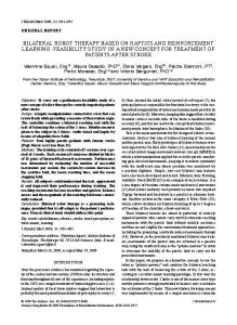
Fig. 3: Three optimal trajectories produced by employing the discovered Pareto optimal solutions. The arrows show the orientation of the AUV (see Section.V-A for more details).

the second surge thruster. However, the other two thrusters are considered fully functional (α1 = α3 = 1). Unlike our previous work [4], our proposed approach benefits from the remaining functionality of the faulty thruster together with the other healthy thrusters. For each experiment we specify a final time, T , for each episode (e.g. T = 60s). The final time is selected somehow that the target is reachable in T seconds. We also designed the vectorized reward function so that when the AUV reaches an area close enough to the desired position, kPt − Pd k < 0.2m, the current episode is terminated. In all the experiments the policy depends on 5 state variables of the system, O = [x y ψ u v] . Employing a 3rd order Fourier basis to represent the features of the policy, the number of optimization parameters is equal to 16 for each thruster. So, for the navigation in 2D plane including 3 thrusters (totally or partially functional ones), the total number of the optimization parameters is 48.

V. IV.

dist < 0.2

Start Point

E XPERIMENTAL R ESULTS

A. A Fully Broken Thruster In the first experiment, we consider the case in which the right surge thruster is fully broken (α2 = 0). In such situation the AUV becomes under-actuated and any attempt to reallocate the actuator configuration matrix would be ineffective. In this scenario, the target is located 4m in front of the AUV and the algorithm tries to find a set of policies to satisfy the multiple-objectives defined in section III-D. The set of optimal trajectories generated by employing the discovered Pareto optimal policies are depicted in Figure 3. The related velocities are shown in Figure 4. The effect of the multiple conflicting objectives can be seen in the figures. For instance, in Figure 3 the final heading error of the AUV with respect to the target in the light blue trajectory is less than the other trajectories. On the other hand, in Figure 4 the light green profile shows a minimum final velocity.

1

0.5

Linear velocity couples u,v

0.5

0.4 0

0.3 −0.5

0.2

0

0.5

1

1.5

2

2.5

3

3.5

4

(a) The solution satisfying the 1st objective, shortest path.

0.1

1

0 0.5

−0.1 0

−0.2 −0.5 0

−0.3

0.5

1

1.5

2

2.5

3

3.5

4

(b) The solution satisfying the 2nd objective, minimum final velocity. −0.4

0

2

4

6

8

10

12

14

16

Time (sec)

Fig. 4: The velocity profiles related to the optimal trajectories in Figure 3. For each trajectory two linear velocity profiles exist (u in x direction, v in y direction) (see Section.V-A for more details).

1

0.5

0

−0.5 0

0.5

1

1.5

2

2.5

3

3.5

4

(c) The solution satisfying the 3rd objective, minimum heading error. 450 50 400 45

B. A Partially Broken Thruster In the second experiment, we consider the case in which the right surge thruster is partially broken (α2 6= 0). In such situation the AUV is considered as redundant, but the dynamic behavior of the system is different. Similar to the previous experiment, the target is located 4m in front of the AUV and the algorithm tries to find a set of optimal policies to satisfy the multiple-objectives defined in section III-D. We repeated this experiment 11 times and each time the coefficient of functionality for the faulty thruster (α2 ) is increased by 0.1 from 0 to 1. The optimal trajectories generated by the discovered Pareto optimal policies in each case are depicted in Figure 5. Since in each experiment, we kept the maximum number of episodes fixed (50), in some cases the algorithm discovered more Pareto optimal policies while in some others it found less solutions. In addition, the maximum number of function evaluations in each case is equal to 1000 times. All the discovered control policies in this experiment are stored in a lookup table and is used in the next experiment. In order to investigate the optimization process in more details, one of the experiments (α2 = 0.4) is repeated with NP = 100,CR = 0.9, Fc = 0.85, Gmax = 50. The results are reported in Figure 6. Three optimal solutions are reported in separate plots (6a, 6b, and 6c). As it can be seen, Figure 6a illustrates a trajectory that satisfies the shortest path objective. The trajectory in Figure 6b satisfies the minimum final velocity and the third trajectory in Figure 6c keeps the heading of the AUV towards the target, to minimize the heading error. In Figure 6d, the reward-space Pareto Front is plotted over the first and third objectives, and the convergence of the populations in each generation is depicted by a color gradient. C. Improving the Performance In future, we plan to evaluate the efficiency of the proposed framework using real-world experiments, similar to our experiments with scalarized objectives in [4]. Therefore, the idea behind this experiment is to benefit from the previous experience and increase the performance of the learning approach by decreasing the computation time. The Pareto optimal

350

40

300

35

250

30 25

200 20 150 15 100

10

50

5

0 0

500

1000

1500

2000

2500

(d) The Pareto Front plotted for two objectives.

Fig. 6: Acquired results for the 2nd experiment with α2 = 0.4. In sub-figures 6a, 6b, 6c the x and y axes show the surge (x) and sway (y) respectively and the dimensions are in meters. In sub-figure 6d, the reward-space Pareto Front is plotted over two objectives, in which the dominant solutions are marked as black. The movement of populations towards minimum rewards is shown with a color gradient. The axis of Figure 6d are dimensionless. (see section V-B for more details.)

solutions for different values of α2 , which are extracted in the previous experiment, are depicted in Figure 7. Each row in Figure 7 is related to a thruster and in each row 16 parameters of the policy θ are depicted. Each θ is plotted versus α (α ∈ [0, 0.1, . . . , 1]). Since the behavior of the parameters seems to be nonlinear, using regression techniques to find a model would be ineffective. Instead, we keep the previous experience as a lookup table for initializing the first generation of parents. We investigate the effect of using previous knowledge by employing the nearest existing solution as initial population. A new experiment is performed where α2 is not exactly one of the previously experienced values. We initialize the approach with the nearest existing solution from the lookup table to increase the efficiency of the approach. In this experiment, α2 = 0.45 is assumed. All the other assumptions are similar to the previous experiments. We first initialize the algorithm with random population to discover an optimal control policy.

1.5

1.5

1

1.5

2

1

= 0.0

2

1

= 0.1

2

0.5

= 0.2

0.5

0.5

0

0

0

0.5

0

0.5

0.5

1

0.5

0

0.5

1

1.5

2

2.5

3

3.5

0

4

1.5

0.5

1

1.5

2

2.5

3

3.5

2

1

0.5

1

1.5

2

2.5

3

3.5

4

2

1

0

= 0.5

2

0.5

= 0.6

0.5

0

0.5

0

0

0.5

0

1

0.5 0

0.5

1

1.5

2

2.5

3

3.5

4

0

0.5

1

1.5

2

2.5

3

3.5

0

4

1

1

2

0.5

= 0.8

2

0.5

= 0.9

0

0.5

0.5

0.5

1

1

1

1.5

2

2.5

3

3.5

4

0.5

2

0.5

0

0.5

1

1.5

2

2.5

3

3.5

4

1

1.5

2

2.5

3

3.5

4

1

1.5

2

2.5

3

3.5

4

1.5

2

2.5

3

3.5

4

= 0.7

0.5 0

0.5

1

0

0

2

1

0.5

0.5

0.5

1.5

1

= 0.4

= 0.3

0.5

0

4

1.5

2

1

= 1.0

1 0

0.5

1

1.5

2

2.5

3

3.5

0

4

0.5

1

Fig. 5: Acquired results for the 2nd experiment with various coefficient of functionality for the right surge thruster which is a dimensionless quantity between [0, 1]. In all sub-figures the x and y axes show the surge (x) and sway (y) respectively in the horizontal plane of AUV and the dimensions are in meters. (see section V-B for more details.)

θ1

θ2

θ3

θ4

θ5

θ6

θ7

θ8

θ9

θ10

θ11

θ12

θ13

θ14

θ15

θ16

Thruster

1

1 0.5 0 −0.5 −1 0 0.5 1 0 0.5 1 0 0.5 1 0 0.5 1 0 0.5 1 0 0.5 1 0 0.5 1 0 0.5 1 0 0.5 1 0 0.5 1 0 0.5 1 0 0.5 1 0 0.5 1 0 0.5 1 0 0.5 1 0 0.5 1 θ1

θ2

θ3

θ4

θ5

θ6

θ7

θ8

θ9

θ10

θ11

θ12

θ13

θ14

θ15

θ16

Thruster

2

0.5 0 −0.5 −1 0 0.5 1 0 0.5 1 0 0.5 1 0 0.5 1 0 0.5 1 0 0.5 1 0 0.5 1 0 0.5 1 0 0.5 1 0 0.5 1 0 0.5 1 0 0.5 1 0 0.5 1 0 0.5 1 0 0.5 1 0 0.5 1 θ1

θ2

θ3

θ4

θ5

θ6

θ7

θ8

θ9

θ10

θ11

θ12

θ13

θ14

θ15

θ16

Thruster

3

1 0.5 0 −0.5 −1 0 0.5 1 0 0.5 1 0 0.5 1 0 0.5 1 0 0.5 1 0 0.5 1 0 0.5 1 0 0.5 1 0 0.5 1 0 0.5 1 0 0.5 1 0 0.5 1 0 0.5 1 0 0.5 1 0 0.5 1 0 0.5 1

Fig. 7: The discovered policy parameters from the 2nd experiment. Each row in the plot is related to a thruster. In each row 16 parameter are depicted (parameters of the policy representation, θ , normalized between −1 and 1). And each parameter is plotted versus α which is a measure of functionality of a thruster. Both axes illustrate dimensionless quantities (see Section.V-C for more details).

Then we repeated the same simulation, starting from the existing optimal solution for α2 = 0.4. To be consistent, both experiments were repeated 20 times. The result is depicted in Figure 8. In the left, the number of function evaluations and in the right, the time to reach the first optimal solution are compared between two cases. All experiments took place on a single thread on an Intel Core i3 CPU 2.30GHz. The result suggests that starting from a neighbour solution can increase the performance of the approach. This result suggests that using such lookup table decreases the computation time efficiently when running the approach on-line.

Fig. 8: This plot shows the effect of employing previously experienced knowledge in the performance of the approach. The first experiment starts from random values, whereas the second experiment uses the nearest neighbor solution. The left plot shows the number of function evaluations and the right plot depicts the time needed to reach the goal. Both experiments were averaged over 20 runs. (see Section.V-C for more details).

VI.

D ISCUSSION AND C ONCLUSIONS

In order to deal with multiple conflicting objectives, a linear scalarization technique was used in our previous work [4]. However, in this paper a multi-objective technique is employed. In linear scalarization technique the objective vector is scalarized according to a weight vector. The weight vector specifies the relative importance of the objectives. Varying weight of an objective will bias the learning towards that objective. One of the disadvantages of scalarization is that the relationship between the policy and the weights may be

unpredictable and small changes in weights may produce large changes in the policy. On the other hand, multi-objective optimization techniques with vectorized objectives address this issue by investigating the nature of Pareto Front for the specified scenario. However, after all they require a decision making algorithm or the user to select the optimal solution. Covering this issue is out of scope of this paper. A model-based direct policy search for discovering faulttolerant control policies for thruster failure recovery in AUVs is proposed. The on-board model of the AUV is first reconfigured according to the detected and isolated fault. The approach learns a fault-tolerant policy and then executes the optimal policy on the AUV. The set of optimal solutions are discovered using a multi-objective reinforcement learning approach. Our framework can deal with both partially and totally broken thrusters. In addition, the proposed approach is applicable when the AUV either becomes under-actuated or remains redundant in the presence of a fault. Finally, the efficiency of the approach is increased by taking advantage of the previous experiences embedded in a lookup table. This capability is useful for further real-world experiments by decreasing the computation time.

[10]

[11]

[12]

[13]

[14]

[15] [16]

[17]

[18]

ACKNOWLEDGMENT This research was supported by the PANDORA EU FP7 project under the grant agreement No. ICT-288273. Website: http://persistentautonomy.com/. R EFERENCES [1]

[2]

[3]

[4]

[5]

[6]

[7]

[8]

[9]

M. Caccia, R. Bono, G. Bruzzone, G. Bruzzone, E. Spirandelli, and G. Veruggio, “Experiences on actuator fault detection, diagnosis and accomodation for ROVs,” International Symposiyum of Unmanned Untethered Sub-mersible Technol, 2001. K. Hamilton, D. Lane, N. Taylor, and K. Brown, “Fault diagnosis on autonomous robotic vehicles with recovery: an integrated heterogeneousknowledge approach,” in Robotics and Automation, 2001. Proceedings 2001 ICRA. IEEE International Conference on, vol. 4. IEEE, 2001, pp. 3232–3237. G. Antonelli, “A survey of fault detection/tolerance strategies for AUVs and ROVs,” in Fault diagnosis and fault tolerance for mechatronic systems: Recent advances. Springer, 2003, pp. 109–127. S. R. Ahmadzadeh, M. Leonetti, A. Carrera, M. Carreras, P. Kormushev, and D. G. Caldwell, “Online discovery of AUV control policies to overcome thruster failure,” in Robotics and Automation (ICRA), 2014 IEEE International Conference on. IEEE, 2014, pp. 6522–6528. S. R. Ahmadzadeh, M. Leonetti, and P. Kormushev, “Online direct policy search for thruster failure recovery in autonomous underwater vehicles,” in 6th International workshop on Evolutionary and Reinforcement Learning for Autonomous Robot System (ERLARS 2013), Taormina, Italy, September 2013. M. Leonetti, S. R. Ahmadzadeh, and P. Kormushev, “On-line learning to recover from thruster failures on autonomous underwater vehicles,” in OCEANS 2013. IEEE, 2013. T. Podder, G. Antonelli, and N. Sarkar, “Fault tolerant control of an autonomous underwater vehicle under thruster redundancy: Simulations and experiments,” in Robotics and Automation, 2000. Proceedings. ICRA’00. IEEE International Conference on, vol. 2. IEEE, 2000, pp. 1251–1256. T. K. Podder and N. Sarkar, “Fault-tolerant control of an autonomous underwater vehicle under thruster redundancy,” Robotics and Autonomous Systems, vol. 34, no. 1, pp. 39–52, 2001. M. Andonian, D. Cazzaro, L. Invernizzi, M. Chyba, and S. Grammatico, “Geometric control for autonomous underwater vehicles: overcoming a thruster failure,” in Decision and Control (CDC), 2010 49th IEEE Conference on. IEEE, 2010, pp. 7051–7056.

[19]

[20] [21]

[22]

[23]

[24]

[25]

[26]

[27]

[28]

[29]

[30]

J.-K. Choi and H. Kondo, “On fault-tolerant control of a hovering AUV with four horizontal and two vertical thrusters,” in OCEANS 2010 IEEESydney. IEEE, 2010, pp. 1–6. S. Koos, A. Cully, and J.-B. Mouret, “Fast damage recovery in robotics with the t-resilience algorithm,” The International Journal of Robotics Research, vol. 32, no. 14, pp. 1700–1723, 2013. D. Perrault and M. Nahon, “Fault-tolerant control of an autonomous underwater vehicle,” in OCEANS’98 Conference Proceedings, vol. 2. IEEE, 1998, pp. 820–824. A. S.-f. Cheng and N. E. Leonard, “Fin failure compensation for an unmanned underwater vehicle,” in Proceedings of the 11th International Symposium on Unmanned Untethered Submersible Technology. Citeseer, 1999. M. L. Seto, “An agent to optimally re-distribute control in an underactuated AUV,” International Journal of Intelligent Defence Support Systems, vol. 4, no. 1, pp. 3–19, 2011. Z. G´abor, Z. Kalm´ar, and C. Szepesv´ari, “Multi-criteria reinforcement learning.” in ICML, vol. 98, 1998, pp. 197–205. S. Mannor and N. Shimkin, “A geometric approach to multi-criterion reinforcement learning,” The Journal of Machine Learning Research, vol. 5, pp. 325–360, 2004. S. Natarajan and P. Tadepalli, “Dynamic preferences in multi-criteria reinforcement learning,” in Proceedings of the 22nd international conference on Machine learning. ACM, 2005, pp. 601–608. D. J. Lizotte, M. H. Bowling, and S. A. Murphy, “Efficient reinforcement learning with multiple reward functions for randomized controlled trial analysis,” in Proceedings of the 27th International Conference on Machine Learning (ICML-10), 2010, pp. 695–702. P. Vamplew, J. Yearwood, R. Dazeley, and A. Berry, “On the limitations of scalarisation for multi-objective reinforcement learning of pareto fronts,” in AI 2008: Advances in Artificial Intelligence. Springer, 2008, pp. 372–378. C. R. Shelton, “Importance sampling for reinforcement learning with multiple objectives,” 2001. L. Barrett and S. Narayanan, “Learning all optimal policies with multiple criteria,” in Proceedings of the 25th international conference on Machine learning. ACM, 2008, pp. 41–47. A. Zhou, B.-Y. Qu, H. Li, S.-Z. Zhao, P. N. Suganthan, and Q. Zhang, “Multiobjective evolutionary algorithms: A survey of the state of the art,” Swarm and Evolutionary Computation, vol. 1, no. 1, pp. 32–49, 2011. R. Storn and K. Price, “Differential evolution–a simple and efficient heuristic for global optimization over continuous spaces,” Journal of global optimization, vol. 11, no. 4, pp. 341–359, 1997. B. Babu and M. M. L. Jehan, “Differential evolution for multi-objective optimization,” in Evolutionary Computation, 2003. CEC’03. The 2003 Congress on, vol. 4. IEEE, 2003, pp. 2696–2703. H. Li and Q. Zhang, “A multiobjective differential evolution based on decomposition for multiobjective optimization with variable linkages,” in Parallel problem solving from nature-PPSN IX. Springer, 2006, pp. 583–592. H. A. Abbass, R. Sarker, and C. Newton, “PDE: a pareto-frontier differential evolution approach for multi-objective optimization problems,” in Evolutionary Computation, 2001. Proceedings of the 2001 Congress on, vol. 2. IEEE, 2001, pp. 971–978. B. Babu and B. Anbarasu, “Multi-objective differential evolution (mode): an evolutionary algorithm for multi-objective optimization problems (moops),” in Proceedings of International Symposium and 58th Annual Session of IIChE. Citeseer, 2005. D. Ribas, N. Palomeras, P. Ridao, M. Carreras, and A. Mallios, “Girona 500 AUV: From survey to intervention,” Mechatronics, IEEE/ASME Transactions on, vol. 17, no. 1, pp. 46–53, 2012. G. C. Karras, C. P. Bechlioulis, M. Leonetti, N. Palomeras, P. Kormushev, K. J. Kyriakopoulos, and D. G. Caldwell, “On-line identification of autonomous underwater vehicles through global derivative-free optimization,” in Proc. IEEE/RSJ Intl Conf. on Intelligent Robots and Systems (IROS), 2013. G. Konidaris, S. Osentoski, and P. S. Thomas, “Value function approximation in reinforcement learning using the fourier basis.” in AAAI, 2011.