Multi-armed bandit experiments in the online service economy Steven L. Scott June 10, 2014 Abstract The modern service economy is substantively different from the agricultural and manufacturing economies that preceded it. In particular, the cost of experimenting is dominated by opportunity cost rather than the cost of obtaining experimental units. The different economics require a new class of experiments, in which stochastic models play an important role. This article briefly summarizes mulit-armed bandit experiments, where the experimental design is modified as the experiment progresses to make the experiment as inexpensive as possible.
Key words: Thompson sampling, sequential experiment, Bayesian, reinforcement learning
1
Introduction
Service is the dominant sector in the United States economy, accounting for roughly 80% of US GDP (World Bank, 2013). It is similarly important in other developed nations. Much activity in the service sector involves traditional retail and person-to-person services, but a growing fraction comes from technology companies like Google, Amazon, Facebook, Salesforce, and Netflix. These and similar companies provide internet services related to search, entertainment, retail, advertising, and information processing under the “software as a service” paradigm. As with other industries, service can be improved through experimentation. Yet service differs in important ways from the manufacturing and agricultural processes that are the focus of traditional industrial experiments. The cost structure of a typical service experiment, particularly online, is dramatically different from that of a manufacturing or agricultural experiment. In the latter, costs arise mainly from acquiring or processing experimental units, such as growing crops on plots of land, destroying items taken from the production line, or paying subjects to participate in a focus group. By contrast, service experiments involve changing the service being provided to existing customers with whom the service provider would have engaged even if no experiment had taken place. Assuming the service can be modified with minimal expense (which is true for online services) then the cost of experimenting is dominated by the opportunity cost of providing sub-optimal service to customers. A second distinction is that service providers are able to continually monitor the quality of the service they provide, for example by keeping track of the number of clicks generated by an 1
advertisement, or the frequency with which a software feature is used. This blurs the line separating the laboratory from the production line, as if the car could be improved after leaving the factory. Online service companies can conduct experiments faster and easier than ever before. Service providers can experiment continuously, perpetually improving different aspects of their offerings (Varian, 2010). One impediment is that experiments are expensive. A dramatic increase in the frequency and scope of experiments requires a corresponding reduction in cost. Multi-armed bandits are a type of sequential experiment that is naturally aligned with the economics of the service industry. This article is a brief introduction to multi-armed bandit experiments, the “Thompson sampling” heuristic for managing them, and some of the practical considerations that can arise in real world applications. Section 2 describes multi-armed bandit experiments and reviews some of the techniques that have been developed to implement them. Section 3 discusses the particular method of Thompson sampling. Section 4 discusses some of the practical aspects of running a multi-armed bandit experiment in various contexts. Section 5 concludes.
2
Multi-armed bandit experiments
A multi-armed bandit is a sequential experiment where the goal is to produce the largest reward. In the typical setup there are K actions or “arms.” Arm a is associated with an unknown quantity va giving the “value” of that arm. The goal is to choose the arm providing the greatest value, and to accumulate the greatest total reward in doing so. The name “multi-armed bandit” is an allusion to a row of slot machines (colloquially known as “one armed bandits”) with different reward probabilities. The job of the experimenter is to choose the slot machine with the highest probability of a reward. A more formal description assumes that rewards come from a probability distribution fa (y|θ), where a indexes the action taken (or arm played), y is the observed reward, and θ is a set of unknown parameters to be learned through experimentation. The value va (θ) is a known function of the unknown θ, so if θ were observed the optimal arm would be known. Consider a few examples for concreteness. 1. In the slot machine problem (the “binomial bandit”) we have θ = (θ1 , . . . , θK ), a vector of success probabilities for K independent binomial models, with va (θ) = θa . 2. In a two-factor experiment for maximizing conversion rates on a web site, suppose the factors are button color (red or blue) and button position (left or right). The experimental configuration can be expressed in terms of two dummy variables Xc (for button color) and Xp (for position). Then θ might be the set of logistic regression coefficients in the model logit P r(conversion) = θ0 + θ1 Xc + θ2 Xp + θ3 Xc Xp .
2
(1)
The action a is isomorphic to the vector of design variables xa = (1, Xc , Xp , Xc Xp ), with va (θ) = logit−1 (θT xa ). 3. As a final example, one could model “restless bandits” (Whittle, 1988) by assuming that some or all the coefficients in equation (1) were indexed by time in a Gaussian process, such as θt+1 = N (θt , Σt ) .
(2)
There are many obvious generalizations, such as controlling for background variation (i.e. the “blocking factors” in a traditional experiment) by including them as covariates in equations (1) or (2), combining information from similar experiments using hierarchical models, or replacing binary rewards with small counts, continuous quantities, or durations. The multi-armed bandit problem is clearly driven by parameter uncertainty. If θ were known then va (θ) would be known as well, and the optimal action would be clear. It is tempting to ˆ find an “optimal” point estimate θˆ and take the corresponding implied action a ˆ = arg maxa va (θ). This is known as the “greedy strategy,” which has been well documented to underperform (Sutton and Barto, 1998). The problem with the greedy strategy is that estimation error in θˆ can lead to an incorrect choice of a ˆ. Always acting according to a ˆ limits opportunities to learn that other arms are superior. To beat the greedy strategy, one must sometimes take different actions than ˆ That is, one must experiment with some fraction of observations. The tension those implied by θ. ˆ and experimenting in case θˆ is wrong is known as between following the (apparently) optimal θ, the “explore/exploit trade off.” It is the defining characteristic of the multi-armed bandit problem. Bandits have a long and colorful history. Whittle (1979) famously quipped that ... [the bandit problem] was formulated during the [second world] war, and efforts to solve it so sapped the energies and minds of Allied analysts that the suggestion was made that the problem be dropped over Germany, as the ultimate instrument of intellectual sabotage. Many authors attribute the problem to Robbins (1952), but it dates back at least to Thompson (1933). For very simple reward distributions such as the binomial, Gittins (1979) developed an “index policy” that produces an optimal solution under geometric discounting of future rewards. The Gittins index remains the method of choice for some authors today (e.g. Hauser et al., 2009). Obtaining optimal strategies for more complex reward distributions such as (1) and (2) is sufficiently difficult that heuristics are typically used in practice. Sutton and Barto (1998) describe several popular heuristics such as �-greedy, �-decreasing, and softmax methods. All of these require arbitrary tuning parameters that can lead to inefficiencies. Auer et al. (2002) developed a popular heuristic in which one selects the arm with the largest upper confidence bound (UCB) of va (θ). For independent rewards with no shared parameters, the UCB algorithm was shown to satisfy the 3
optimal rate of exploration discovered by Lai and Robbins (1985). Agarwal et al. (2009) used UCB to optimize articles shown on the main Yahoo! web page. More recently, attention has been given to a technique known as Thompson sampling. Chapelle and Li (2011) produced simulations showing that Thompson sampling had superior regret performance relative to UCB. See Scott (2010) for comparisons to older heuristics. Thompson sampling is the method used in the remainder of this article.
3
Thompson sampling
Thompson sampling (Thompson, 1933) is a heuristic for managing the explore/exploit trade-off in a multi-armed bandit problem. Let yt denote the set of data observed up to time t, and define wat = P r(a is optimal|yt ) Z = I(a = arg max va (θ))p(θ|yt ) dθ.
(3)
The Thompson heuristic assigns the observation at time t + 1 to arm a with probability wat . One can easily compute wat from a Monte Carlo sample θ(1) , . . . , θ(G) simulated from p(θ|yt ) using G
wat ≈
1 X I(a = arg max va (θ(g) )). G
(4)
g=1
Notice that the algorithm where one first computes wat and then generates from the discrete distribution w1t , . . . , wKt is equivalent to selecting a single θt ∼ p(θ|yt ) and selecting the a that maximizes va (θt ). Thus Thompson sampling can be implemented using a single draw from p(θ|y), although computing wat explicitly yields other useful statistics such as those described in Section 3.1. The Thompson heuristic strikes an attractive balance between simplicity, generality, and performance. Perhaps most importantly, it is easy to understand. If arm a has a 23% chance of being the best arm then it has a 23% chance of attracting the next observation. This statement obscures technical details about how the 23% is to be calculated, or why the two probabilities should match, but it contains an element of “obviousness” that many people find easy to accept. If desired, tuning parameters can be introduced into Thompson sampling. For example one could assign observations γ with probability proportional to wat . Setting γ < 1 makes the bandit less aggressive, increasing
exploration. Setting γ > 1 make the bandit more aggressive. Of course, exploration can also be encouraged by introducing a more flexible reward distribution, for example replacing the binomial with the beta-binomial. Section 4 discusses reward distributions that can be used for controlling exploration, which can be more effective than tuning parameters. Modifying the reward distribution to slow convergence highlights a second feature of Thompson sampling, which is that it can be applied generally. The only requirement is the ability to simulate θ from p(θ|yt ), which can be 4
done using standard Bayesian methods for a very wide class of reward distributions. Thompson sampling handles exploration gracefully. Let a∗t = arg maxa wat denote the arm with the highest optimality probability given data to time t. The fraction of data devoted to exploration at time t + 1 is 1 − wa∗t t , which gradually diminishes as the experiment evolves. Thompson sampling not only manages the overall fraction of exploration, it manages exploration at the level of individual arms. Clearly inferior arms are explored less frequently than arms which might be optimal, which has two beneficial implications. First, it improves the economic performance of the experiment and offers customers who would have been assigned to inferior arms a better experience. Second, it produces greater sample sizes among arms near the top of the value scale, which helps distinguish the best arms from the merely good ones. Thompson sampling tends to shorten experiments while simultaneously making them less expensive to run for longer durations. The randomization in Thompson sampling is an often overlooked advantage. In practice, online experiments can involve many (hundreds or thousands) of visits to a web site before updating can take place. It is generally preferable to update as soon as possible, but updates may be delayed for technical reasons. For example, the system that logs the results of site visits might be different from the system that determines which version of the site should be seen. It can take some time (several minutes, hours, or perhaps a day) to collect logs from one system for processing in another, and during that time a high-traffic site might attract many visitors. Thompson sampling randomly spreads observations across arms in proportion to wat while waiting for updates. Non-randomized algorithms pick a single arm, making the same “bet” for each experimental unit, which substantially increases the variance of the rewards. (Rewards are great if you bet on the right arm, and terrible if you bet on the wrong one.) Randomization also offers a source of pure variation that can help ensure causal validity. Although Thompson sampling does not explicitly optimize a specific criterion, there are mathematical and empirical results showing that it tends to beat other heuristics. Chapelle and Li (2011) produced a highly cited simulation study showing that Thompson sampling outperformed UCB in the case of the binomial bandit. May et al. (2012) showed that Thompson sampling is a consistent estimator of the optimal arm, and over the life of the experiment “almost all” (in a probabilistic sense) of the time is spent on the optimal arm. Kaufmann et al. (2012) showed that Thompson sampling for the binomial bandit satisfies the Lai and Robbins (1985) optimal bound. Bubeck and Liu (2013a,b) have established regret bounds for Thompson sampling in the case of independent arms with rewards in [0, 1].
3.1
Using regret to end experiments
The methods used to compute wat for Thompson sampling can also produce a reasonable method of deciding when experiments should end.
Let θ0 denote the true value of θ and let a∗ =
arg maxa va (θ0 ) denote the arm that is truly optimal. The regret from ending the experiment
5
at time t is va∗ (θ0 ) − va∗t (θ0 ), which is the value difference between the truly optimal arm and the arm that is apparently optimal at time t. In practice regret is unobservable, but we can compute its posterior distribution. Let v∗ (θ(g) ) = maxa va (θ(g) ) where θ(g) is a draw from p(θ|yt ). Then r(g) = v∗ (θ(g) ) − va∗t (θ(g) ) is a draw from posterior distribution of regret. Note the distinction: v∗ (θ(g) ) is the maximum value available within Monte Carlo draw g, while va∗t (θ(g) ) is the value (again in draw g) for the arm deemed best across all Monte Carlo draws. Their difference is often 0, but is sometimes positive. For communication purposes, it is helpful that the units of regret are the units of value (e.g. dollars, clicks, or conversions). The distribution of regret can be summarized by an upper quantile, such as the 95th percentile, to give the “potential value remaining” (PVR) in the experiment. PVR is the value per play that might be lost if the experiment ended at time t. Because businesses experiment in the hope of finding an arm that provides greater value, a sensible criterion for ending the experiment is when PVR falls below a threshold of practical significance. In addition to dealing directly with the question at hand, the PVR statistic handles ties gracefully. If there are many arms in the experiment there can be several that give essentially equal performance. This could easily happen in a multi-factor experiment where one factor was irrelevant. Experiments ended by the PVR criterion naturally produce two sets of arms: one that is clearly inferior, and a second containing arms that are nearly equivalent to one another. Any arm from the set of potential winners can be chosen going forward. If desired, one may use wat as a guide for choosing among the potential winners, but subjective preference (e.g. for an existing version) may be used as well. Note that regret can also be defined as a percentage change from the current apparently optimal arm, so that draws from the posterior are given by ρ(g) =
v∗ (θ(g) ) − va∗t (θ(g) ) , va∗t (θ(g) )
(5)
which is unit-free. If the experimenter is unwilling to specify a definition of “practical significance,” then an experimental framework can use an arbitrary operating definition such as ρ < .01.
4
Practical applications of Thompson sampling
This Section discusses some of the practicalities associated with implementing Thompson sampling in applied problems. It begins with a simulation study showing the gains from Thompson sampling relative to traditional experiments, before turning to a set of useful generalizations.
6
40 0
20
Frequency
60
10 20 30 40 50 60 70 0
Frequency
0
1
2
3
4
5
0
Millions of observations
50
100
150
200
Lost conversions
(a)
(b)
Figure 1: (a) Histogram of the number of observations required in 100 runs of the binomial bandit described in Section 4.1. (b) The number of conversions lost during the experiment period. The vertical lines show the number of lost conversions under the traditional experiment with 95% (solid), 50% (dashed), and 84% (dotted) power.
4.1
A/B Testing
Among internet companies, the term “A/B testing” describes an experiment comparing a list of alternatives along a single dimension, which statisticians would call the “one way layout”. An A/B test often involves only two alternatives, but the term is sometimes sloppily applied to experiments with multiple alternatives. A canonical example of A/B testing is website optimization, where multiple versions of a web site are constructed, traffic is randomly assigned to the different versions, and counts of conversions are monitored to determine which version of the site performs the best. A “conversion” is an action designated by the site owner as defining a successful visit, such as making a purchase, visiting a particular section of the site, or signing up for a newsletter. Consider two versions of a web site that produce conversions according to independent binomial distributions. Version A produces a conversion 0.1% of the time (p = .001) and version B produces conversions 0.11% of the time (p = .0011). To detect this difference using a traditional experiment with 95% power under a one-sided alternative we would need roughly 4.5 million observations (2,270,268 in each arm). If we decreased the power to .5 we would need slightly more than 1.1 million (567,568 in each arm). The regret for each observation assigned to version A is .0011−.001 = .0001, so for every 10,000 observations assigned to version A we lose one conversion. Figure 1 shows the results from simulating the multi-armed bandit process 100 times under
7
the conditions described above. Each simulation assumes the site receives 100 visits per day. The true success probabilities are held constant across all simulation runs. Observations are assigned to arms according to the Thompson procedure with updates occurring once per day (so there are 100 observations per update). Each simulated experiment was ended when the potential value remaining statistic in equation (5) fell below ρ = 1%. The simulation found the correct version in 84 out of 100 runs. Figure 1(a) shows that the number of observations required to end the experiment is highly variable, but substantially less than the numbers obtained from the power calculations for the traditional experiments. Figure 1(b) compares the number of lost conversions, relative to the optimal policy of always showing version B, for the bandit and for the traditional experiments with power .5, .84 (the realized power of this simulation), and .95. Roughly 2/3 of the simulation runs resulted in single digits of lost conversions compared to hundreds of lost conversions for the traditional experiment with comparable power. Given that this artificial “site” generates about 1 conversion every 10 days, 100 conversions is a staggering difference. The savings are partly due to shorter experiment times, and partly due to the experiments being less expensive while they are run. Both factors are important. Under the 95% power calculation the experiment would take roughly 125 “years,” while 29 of 100 bandit simulations finished within one “year”. Both are impractically long, but the bandit offers at least some chance of completing the experiment. Detecting small differences is a hard problem, made harder when the baseline probabilities are small as well. Scott (2012) gives similar results for an easier setting with true success rates of 4% and 5%, and for settings with multiple arms. When there is a difference to be found, the multi-armed bandit approach is dramatically more efficient at finding the best arm than traditional statistical experiments, and its advantage increases as the number of arms grows (Berry, 2011).
4.2
Contextual information
The multi-armed bandit can be sensitive to the assumed model for the rewards distribution. The binomial model assumes all observations are independent with the same success probability. In practice this assumption can fail if different arms are exposed to sub-populations with different performance characteristics at different times. For companies with an international web presence this can appear as a temporal effect as Asian, European, and American markets become active during different times of the day. It can also happen that people browse in different modes on different days of the week, for example by researching an expensive purchase during lunch hours at work but buying on the weekends. Now suppose an experiment has two arms, A and B. Arm A is slightly better during the week when people browse but tend not to buy. Arm B is much better during the weekend, when people buy. With enough traffic it is possible for the binomial model to conclude that A is the superior arm prior to seeing any weekend traffic. This is a possibility regardless of whether the experiment is run as a bandit or as a traditional experiment, but the bandit experiment is more susceptible
8
because it will be run for a shorter period of time. There are two methods that can be used to guard against the possibility of being misled by distinct sub-populations. If the specific sub-populations are known in advance, or if a proxy for them such as the geographically induced temporal patterns is known, then the binomial model can be modified to a logistic regression logit(pa|x ) = β0a + β T x
(6)
where x is a set of variables describing the context of the observation, pa|x is the success probability if arm a is played during context x, β0a is an arm specific coefficient (with one arm’s coefficient set to zero), and β is a set of coefficients for the contextual data to be learned as part of the model. The value function may be taken to be va (θ) = logit−1 (β0a ). If the important contexts are unknown then one may choose to assume that contexts occur as random draws from a distribution of contexts, such as in the beta-binomial hierarchical model, θat ∼ Be(αa , βa ) yt |a ∼ Bin(θat ).
(7)
The model parameters here are θ = {αa , βa : a = 1, 2, . . . , K}, with value function va (θ) = αa /βa . Model (6) will give less “credit” to an arm that produces a conversion inside a context where conversions are plentiful, and more in contexts where conversions are rare. Model (7) will continue exploring for several update periods, even if arm a is dominant in the early periods, to guard against the possibility that the advantage in the early periods was simply the result of random variation at the θat level.
4.3
Personalization
The models in equations (6) and (7) purposefully omit interactions between contextual variables and experimental factors because they are intended for situations where the experimental goal is to find a global optimum. Interactions between contextual and design variables allow for the possibility that the optimal arm may differ by context. For example, one version of a page may perform better in Asia while another performs better in Europe. Depending on the granularity of the contextual data available this approach may be used to personalize results down to the individual level. Similar approaches, though not necessarily using Thompson sampling, are being used in the context of personalized medicine (Chakraborty and Moodie, 2013).
4.4
Multivariate testing
Internet companies use the term “multivariate testing” to describe an experiment with more than one experimental factor. Statisticians would call this the “multi-way layout” or simply a “designed 9
experiment.” Scott (2010) showed how a multi-factor experiment can be handled using Thompson sampling with a probit regression model analogous to equation (1). Fractional factorial designs (e.g. Box, Hunter, and Hunter, 2005) are a fundamental tool for handling traditional multi-factor experiments. Fractional factorial designs work by finding a minimal set of design points (i.e. rows in a design matrix) that allow a pre-specified set of main effects and interactions to be estimated in a linear regression. The equivalent for a multi-armed bandit experiment is to specify a set of main effects and interactions to be estimated as part of the reward distribution. Spike and slab priors can be used to select which interactions to include (Box and Meyer, 1993). In a manufacturing experiment, each distinct configuration of experimental units involves changing the manufacturing process, which is potentially expensive. Thus, having a design matrix with a minimal number of unique rows is an important aspect of traditional fractional factorial experiments. In an online service experiment different configurations can be generated programmatically, so it is theoretically possible to randomize over all potential combinations of experimental factors. The restricted model helps the bandit because there are fewer parameters to learn, but the constraint of minimizing the number of design points is no longer necessary.
4.5
Large numbers of arms
Many online experiments involve online catalogs that are too large to implement Thompson sampling as described above. For example, when showing ads for commodity consumer electronics products (e.g. “digital camera”) the number of potential products that could be shown is effectively infinite. With infinitely many arms, attempting to find the best arm is hopeless. Instead, the decision problem becomes whether or not you can improve on the arms that have already been seen. This problem has been studied by Berry et al. (1997), among others. One approach to the problem is as follows. Consider the infinite binomial bandit problem, and assume that the arm-specific success probabilities independently follow θa ∼ Be(α, β). Suppose Kt arms have been observed at time t. One can proceed by imagining a Kt + 1 armed bandit problem, where success probabilities for Kt of the arms are determined as in Section 4.1, but success probabilities for the “other arm” are sampled from the prior. If the “other arm” is selected by the Thompson heuristic then sample an as-yet unseen arm from the catalog. A similar hierarchical modeling solution can be applied to context-dependent or multivariate problems by assuming the coefficients of the design variables with many levels are drawn from a common distribution, such as a Gaussian or t. The amount of exploration can be increased by increasing the number of draws from the prior at each stage.
10
5
Conclusion
Multi-armed bandit experiments can be a substantially more efficient optimization method than traditional statistical experiments. The Thompson sampling heuristic for implementing multiarmed bandit experiments is simple enough to allow flexible reward distributions that can handle the kinds of issues that arise in real applications. Business and science have different needs. Traditional experiments were created to address uncertainty in scientific problems, which is a naturally conservative enterprise. Business decisions tend to be more tactical than scientific ones, and there is a greater cost to inaction. The two business sectors that dominated the 20th century, agriculture and manufacturing, happen to have economic structures that align with scientific conservatism, which partly explains why they succeeded so well using the tools of science. In those sectors a type I error is costly because it means a potentially expensive change to a production environment with no accompanying benefit. In the service economy type I errors are nearly costless, so artificially elevating them over expensive type II errors makes very little sense. When paired with the fact that the proportion of type I errors is bounded by the proportion of true null hypotheses, the significance vs. power framework underlying traditional statistical experiments seems a poor fit to the modern service economy. By explicitly optimizing value, multi-armed bandits match the economics of the service industry much more closely than traditional experiments, and should be viewed as the preferred experimental framework. This is not to say that there is no room for traditional experiments, but their use should be limited to high level strategic decisions where type I errors are truly important.
References Agarwal, D., Chen, B.-C., and Elango, P. (2009). Explore/exploit schemes for web content optimization. In Proceedings of the 2009 Ninth IEEE International Conference on Data Mining, 1–10. IEEE Computer Society Washington, DC, USA. Auer, P., Cesa-Bianchi, N., and Fischer, P. (2002). Finite-time analysis of the multiarmed bandit problem. Machine Learning 47, 235–256. Berry, D. A. (2011). Adaptive clinical trials: The promise and the caution. Journal of Clinical Oncology 29, 606–609. Berry, D. A., Chen, R. W., Zame, A., Heath, D. C., and Shepp, L. A. (1997). Bandit problems with infinitely many arms. The Annals of Statistics 25, 2103–2116. Box, G. and Meyer, R. D. (1993). Finding the active factors in fractionated screening experiments. Journal of Quality Technology 25, 94–94. Box, G. E., Hunter, J. S., and Hunter, W. G. (2005). Statistics for experimenters. Wiley New York. Bubeck, S. and Liu, C.-Y. (2013a). A note on the Bayesian regret of Thompson sampling with an arbitrary prior. arXiv preprint arXiv:1304.5758. 11
Bubeck, S. and Liu, C.-Y. (2013b). Prior-free and prior-dependent regret bounds for Thompson sampling. In C. Burges, L. Bottou, M. Welling, Z. Ghahramani, and K. Weinberger, eds., Advances in Neural Information Processing Systems 26, 638–646. Curran Associates, Inc. Chakraborty, B. and Moodie, E. E. M. (2013). Statistical Methods of Dynamic Treatment Regimes. Springer. Chapelle, O. and Li, L. (2011). An empirical evaluation of Thompson sampling. In Neural Information Processing Systems (NIPS). Gittins, J. C. (1979). Bandit processes and dynamic allocation indices. Journal of the Royal Statistical Society, Series B: Methodological 41, 148–177. Hauser, J. R., Urban, G. L., Liberali, G., and Braun, M. (2009). Website morphing. Marketing Science 28, 202–223. Kaufmann, E., Korda, N., and Munos, R. (2012). Thompson sampling: an asymptotically optimal finite time analysis. In International Conference on Algorithmic Learning Theory. Lai, T.-L. and Robbins, H. (1985). Asymptotically efficient adaptive allocation rules. Advances in Applied Mathematics 6, 4–22. May, B. C., Korda, N., Lee, A., and Leslie, D. S. (2012). Optimistic bayesian sampling in contextualbandit problems. The Journal of Machine Learning Research 13, 2069–2106. Robbins, H. (1952). Some aspects of the sequential design of experiments. Bulletin of the American Mathematical Society 58, 527–535. Scott, S. L. (2010). A modern Bayesian look at the multi-armed bandit. Applied Stochastic Models in Business and Industry 26, 639–658. (with discussion). Scott, S. L. (2012). Google Analytics help page. https://support.google.com/analytics/ answer/2844870?hl=en. Sutton, R. S. and Barto, A. G. (1998). Reinforcement Learning: an introduction. MIT Press. Thompson, W. R. (1933). On the likelihood that one unknown probability exceeds another in view of the evidence of two samples. Biometrika 25, 285–294. Varian, H. R. (2010). Computer mediated transaction. American Economic Review: Papers and Proceedings 100, 1–10. Whittle, P. (1979). Discussion of “bandit processes and dynamic allocation indices”. Journal of the Royal Statistical Society, Series B: Methodological 41, 165. Whittle, P. (1988). Restless bandits: Activity allocation in a changing world. Journal of Applied Probability 25A, 287–298. World Bank (2013). http://data.worldbank.org/indicator/NV.SRV.TETC.ZS/countries/ 1W-US?display=default.
12