Mobility Impact on Mobile Ad hoc Routing Protocols Nadjib Badache,

Djamel Djenouri

Abdelouahid Derhab,

Basic software laboratory, CERIST, 3 Aissou brothers road, Ben-aknoun, Algiers, Algeria [email protected]

Basic software laboratory, CERIST, 3 Aissou brothers road, Ben-aknoun, Algiers, Algeria [email protected]

Basic software laboratory, CERIST, 3 Aissou brothers road, Ben-aknoun, Algiers, Algeria [email protected]

Abstract An ad hoc network is a set of mobile units connected by wireless technologies, making an infrastructureless temporary network. without turning to a central administration. The network topology is unpredictable, dynamic, it may change any time. These topology changes make ad hoc networks challenging to implement routing protocols. In this paper, we study mobility effects on the performance of several mobile ad hoc routing protocols. Keyw ords Ad Hoc mobile networks, wireless networks, routing protocols, simulation, GloMoSim.

The reactive protocols create routes only if needed by the source node; the disadvantage with this approach is that the delay to obtain routes may be high. In this paper we present some parameters and metrics that we have added to Glomosim, and we study mobility effects on the performance of six protocols, four reactive (ABR, AODV, DSR, LAR) and two proactive (FSR, WRP) by measuring different quantitative metrics at different mobility levels. The remainder of the paper is organised as follows: Section 2 presents an overview of the routing protocols simulated. Section 3 presents metrics and parameters added to the simulator. Section 4 contains the results of our simulation experiments. Finally, a conclusion is presented in Section 5.

1 INTRODUCTION

2 PROTOCOLS OVERVIEW

Ad hoc mobile networks are dynamically formed by a set of mobile nodes connected by wireless links without any predefined infrastructure or centralised administration. It can be used in different applications such as: emergency search and rescue operations, communication between soldiers on a battlefield, sharing information in conference, and data acquisition operations in inhospitable terrains. In such networks, a pair of nodes communicates by sending messages either over a direct wireless link, or over a sequence of wireless links including one or more intermediate nodes (hops). A wireless link is established only if two nodes are within a certain transmission radius called power range. In order to provide communication within the networks, a routing protocol is used to discover routes between nodes. An ad hoc network routing protocol must deal with many limitations, which include frequent topology changes, low battery lives , low bandwidth, and high error rates. Implementing routing protocol that establishes an efficient route between a pair of nodes in such environment is one of the challenges facing ad hoc mobile networks. Ad hoc network routing protocols can be divided in two categories: the proactive protocols and the reactive protocols. The proactive protocols maintain permanently for each node, routes to every other nodes in the network. This approach is costly in terms of resources such as bandwidth, battery power and CPU.

0-7803-7983-7/03/$17.00 ©2003 IEEE

2.1 WPR (Wireless Routing Protocol) [6] WRP is based on a vector distance algorithm. To avoid counting to infinity problem, WRP introduces the shortest way predecessor node for each destination. Each node maintains 4 tables : distance table, routing table, link cost table and Message Retransmission List (MRL). When a node either detects a neighbour link state change, or receives an update message from its neighbours, it sends another update message. Nodes included in response list of the update message (formed using MRL), have to acquit the message reception. If there is no routing table change compared with the last update, node has to send a hello message to ensure the connection. At the time of update message reception, node modifies its distance and seeks best routes basing on the received information. MRL list, must be updated after each ACK reception. 2.2 FSR (Fisheye State Routing) [7] FSR is based on the fisheye technique [3], in order to reduce topological information size. Intuitively, this technique gives a great precisions at a focal point, then this precision regarding a given node decreases when distance between this node and the focal one increases. FSR protocol is similar to the LS (Link State) approach, as each node saves the whole topology. The main difference is the manner in which routing information are exchanged between nodes. In FSR

there is no message flooding, so that control messages are exchanged only between neighbours. 2.3 DSR (Dynamic Source Routing) [2] Each node keeps in its cache the source routes learned. When it needs to send a packet, it checks its cache first, then if it finds a route to the corresponding destination, it uses it, else it broadcasts a request packet through the network. When receiving request packet, a node seeks a route in its cache, if it finds it, it sends a reply packet to the source, else it adds its address to the request packet, and continue the broadcasting. When a node detects a route failure, it sends an error packet to the source, then this one applies again route discovery process. 2.4 AODV (Ad hoc On-Demand Vector) [8]

Distance

When a node need to send a data packet to a destination, it has to broadcast a request packet to all its neighbours, then each neighbour do so, until reaching the destination node. This one sends a reply packet that travels the inverse path until the source, so that a route between the source and the destination is built. 2.5 ABR (Associativity Based Routing) [9] ABR is based on nodes’ associativity, a new metric known as “ associativety degree” is used, a route is chosen depending on associativity state between nodes. Each node sends periodically a special control message called “ Beacon”. When a neighbour node receives this Beacon, it increases its associativity value regarding to the sender. The associativity value becomes null when a node loses its link with the corresponding neighbour. Where a node needs to send a message to a destination, it broadcasts a BQ (Broadcast query) request. At the time of BQ reception, an intermediate node adds its address and its associativity degree to BQ. Destination node chooses the best route depending on associativity degrees, then sends a reply to the source. A source motion causes a new BQ-RPLY process. When a link fails, due to destination or intermediate nodes mobility, a Local-Query packet (LQ[H]) is sent, when H is the hops number till the destination), is sent. When the destination receives this packet, it chooses the best partial route, then sends it to LQ[H] packet sender. 2.6 LAR (Location Aided Routing) [4] LAR seems to DSR, except that it is based on localization. Its purpose is to limit route request packets broadcast. So it uses GPS’ (Global Positioning System) localization information.

3 SIMULATION ENVIRONMENT In this paper we evaluate six protocols, four reactive : ABR, DSR, AODV, LAR and two proactive : FSR and WRP. We use GloMoSim simulator [10]. For our simulation purposes, we have extended GloMoSim by adding ABR protocol and other parameters and metrics implementations. Our simulation environment is characterised by the following parameters: Mobility model: Among GloMoSim’s mobility models, we have chosen the waypoint one, that is the closest to real motion. In this model, a node selects randomly a destination from the physical area, then it moves to this destination, where it stays for a giving time, then it repeat this process. Surface area: The chosen area is 1600m × 400m. Propagation model : We have chosen Free Space model, which supposes that there is no obstacles between a sender and a receiver. The signal dim is proportional to the distance between them. This is a simple model, it eliminates obstacles effect during simulation.

We have chosen for this layer IEEE 802.11 protocol, it is largely used in wireless networks and has the following advantages:

MAC layer protocol :

•

Each transmission is followed by a reply when the packet is correctly received by the destination. • The absence of a Reply after several sends means that the link between two nodes is failed. • It uses a buffer to save packets, even if the system is idle. Application layer: We used in this layer, CBR (Constant Bit Rate) application. 3.1 Constants used Constants are divided into two categories: first those specific to each protocol, and second common constants A) Specific constants Table 1: DSR Constants Time between 2 transmissions of the same request Waiting time for a non broadcasting request Route conservation time in the cache Maximum route length

500 ms 30 ms 30 s 9

Table 2:AODV Constants Route conservation time in the routing table Request retransmissions number Time before deleting a failed link from routing table

10 s 2 4.2 s

Table 3: FSR Constants Intra scope (Update period in the first reach)

5s

Inter scope (Update period in the second reach)

15 s

n Ax(t )− Ax (t + ∆t) Mx= ∑ T t =0 n dist(nx ,ni ) Ax(t)= ∑ n−1 i=1

Maximum route length

9

Maximum number of sequence number

1024

Request life-time

30 s

Table 5: ABR Constants Time between 2 beacons sends

1s

Waiting time before resend a request if there is no reply arrived Time between 2 neighbours presence verifications

500 ms

Waiting time before selecting route

100 ms

4.5 s

Table 6: WRP Constants 2s

b) Common constants Data packet size : 1 Ko Data packet transfer rate : 1 Packet/s Nodes number : 50 Simulation time : 15 Minutes Pause time : 1 second 3.2 Mobility definition Mobility is an important parameter in ad hoc routing protocols evaluation, because of frequent topology changes. There are many definitions of this parameter, such as node speeds or pause time in waypoint model. These definition are meaningless, nodes may move either in a high speed or a low pause time towards the same direction, without any topology change, on the other hand, they may have a low speed or high pause time, but they moves away from each other. For statement let consider a network consisting of 2 linked nodes, that move with a high speed and/or a low pause time, but towards a same direction, so the 2 nodes still linked. But if they move with a low speed and/or a high pause time away one from each other, after a given time, the link will be failed. This example illustrates the meaningless of explaining mobility by nodes’ speed or pause time. A more suitable mobility definition is presented in [5]. This definition is based on relative nodes’ movement; that expresses better network topological change. Mobility is a function of both a speed and movement pattern, it is represented by a new parameter called (mobility factor) that is computed during the

T − ∆t

where : dist(nx,ny) : Distance between node x and node y. n : nodes number. Ax(t) : average distance between node x and all the others nodes, at time t. Mx : average relative mobility of node x, regarding all other nodes, during simulation time. T : simulation time. ∆ t : time period used in calculation. We calculate Ax (t) after each ∆ t, that means we do it for t=0, t= ∆ t, t=2 ∆ t,………….,t=T. For our simulation, we have added to GloMoSim as well mobility factor computation, as an other parameter (INTERVALTIME) that can be specified in the input file, in order to give a value to ∆ t. To the validity of this parameter, we added average link changes number computation during simulation, a change may be either a new link creation or a link failure. we define average link changes computation LINK_CHANG by the following formula : LINK_ CHANG=

t ∑ link _ change(t )× ∆ T T

t= ∆t

Link_change(t) n−1 n

=

∑ ∑[state(t ,i , j)⊕ state(t −∆ t,i, j )]

i= 0 j= i+1

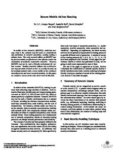
1 if i is linked with j at time t, state(t ,i ,j) = 0 otherwise variation of links changes number regarding mobility is represented in figure 1 average number of link changes

2s 128 By te

Time between 2 Hello messages

n

Mob= ∑ M i i=1

Table 4: LAR Constants Time between 2 transmissions of the same request Buffer length

simulation, with certain rate ∆ t. Mobility factor is given by the following formula :

300 200 100 0 0

2

4

6

8

mobility factor

Figure1 relation between mobility and links changes number

3.3 Computed metrics

c) overhead

Protocols comparison will be carried out by dealing with five metrics, that we consider to be relevant, in different conditions. Then we observe their effect on the network. These parameters are:

It is the number of packets generated by the routing protocol during the simulation, formally speaking it is:

a) Data reception rate It is the number of received packets divided by the number of sent packets at application layer level. It is an important parameter, it is even the most important one in our comparison. More this parameter’s value approach to 1, more the lost packets number is reduced, which imply that the protocol is reliable (regarding this metric). On the other hand, if the value stray from 1, lost packets number increases. b) Consumed energy because energy resources in wireless networks are limited, a protocol is as better as it needs less energy consumption compared with others in the same conditions. Energy computation have already been implemented in GloMoSim using NCR Wavelan radio model. Consumed energy computation of a node i (Power_consumed i) formula is the following: Power_consumedi=

∑trans _delay×(RRR − RSR)

+

reception

∑trans _ delay(RTR− RSR) +

transmission

n

overhead =

∑overheadi where: i=1

overheadi is control packets number generated by node i. Generation of an important overhead will, no doubt, cause buffers congestion from network layer, and bandwidth occupation when sending these control packets. Although control packets are necessary to ensure protocol functioning, their number should not be very large. d) Average data packet transfer delay It is average time separating data packets sending from source nodes and their arriving at destination ones, in the application layer. If we note this metric by delay, we will have: delay =

delayi ∑ nbr_ pr i∈pr

pr: is the set of packets received by all destination nodes. nbr_pr : is the received packets number delayi : is the transfer delay of packet i, such as: delayi = packet i arrival time – packet i send time. This metric is very important for studding protocol quality of service. In case of real time application, this metric estimation have an essential part to select a protocol.

RSR× (radio_ turnOffTime− radio _turnOnTime) e) Paths’ optimality where : trans_delay = packet size / bandwidth + synchronizationTime synchronisation time: constant equal to 192 micro second RTR(radio_transmission_rate) = 3/second RRR(radio_reception_rate) = 1.48/second RSR(radio_sleep_rate) = 0.18/second Radio_turnOnTime: the radio turning on time (simulation start) Radio_turnOffTime: the radio turning off time (simulation end) In our study, we are not interested in consumed energy for each node, but we are interested in average consumed energy in the network, so we added this metric (average_power) calculation, presented by the following formula:

power _consumedi n i=1 n

average_power =

∑

It represents average difference between covered path, and optimal path. We have added to the simulator in network layer level, a mechanism independent of routing protocols, that calculates for each data packet the optimal path between source and destination, before sending it to the MAC layer. It saves this path length (hops number), in IP header of the packet. At each hop, another field , that is initially null, will be increased in order to indicate covered path length. When it arrives at its final destination, difference between covered path and the optimal one, will be computed. Let us note opti the difference between optimal path and the one covered by the packet, and opt our metric, the computation formula is: opt =

opti ∑ nbr_ pr i∈pr

optimal path calculation is carried out basing on width graph exploring algorithm [1], this algorithm calculates optimal path between a given node (r) and all the others in the network, but we are only interested in the path between a source and a destination. So in the implementation, we stop processing when we arrive to the target destination.

4 SIMULATION RESULTS In the following tests, we vary mobility factor, in order to see its impact on measured metrics. The purpose of these simulations is to show mobility variation effects on metrics defined before. Each metric is calculated as well for proactive protocols as for reactive ones. We set along all simulation : the CBR source number to 16, and the power range to 250 m 4.1 Data reception rate (drr) In figure 2.a we see that drr in AODV and LAR still relatively stable for all mobility values, it is more than 84% for AODV and 94% for LAR when mobility is 8 m/min. On the other hand, ABR’s and DSR’s drr decreases when mobility increases. We point out that ABR has a slightly better drr than DSR for high mobility, and we remark that both ABR and DSR have important data loses, they beyond 40% in the case of average and high mobility values. The raison for this is: first, for ABR, associativity propriety supposes that a path with higher associativity value, will be more long-lived. This supposition is meaningless when mobility increases. Then chosen routes are not necessary the most stable. Second, for DSR, link failure are detected just when sending a data packet via a failed link, this packet will be lost if the link detector node has no route to the packet destination. On the other hand AODV react more quickly to link failures, by sending an error packet to active neighbours as soon as it receives error message from its MAC layer. In figure 2.b we remark that both WRP and FSR lose a great amount of data packets since a low mobility (1 m/min), and the lost keeps increasing when mobility increases, and may exceed 60%. In vicinity of mobility 0, both proactive and reactive protocols give a good drr, but from mobility 1 m/min, which is relatively low, proactive’s drr decrease disastrously . that is because packets are sent before routing tables converge to a stable state, then they take failed routes supposed be valid. 4.2 Average data packet transfer delay In figure 3.a we see that ABR, AODV and DSR have low transfer delays and they are not so influenced by mobility rise. On the other hand, more the mobility rises, more LAR’s average delay increases, and may go down to 160 ms when the mobility value is high. In the case of high mobility , GPS information are more and more wrong. So partial propagation route discovery of LAR (that broadcasts request in a limited area), often fails. Discovery will be affected after a global broadcast, that causes a high transfer delay.

In figure 3.b we note that delay is steady, it varies from 8 to 24 ms, and mobility has not a meaningful effect. Delays of proactive protocols are smaller and more stable than those of reactive ones . Proactive protocols unlike reactive ones, construct and maintain routing tables permanently, that eliminates route discovery time. But we point out that this results are however misleading, because proactive protocols drop so many packets. And these packets are not included in the average delay calculation. 4.3 Overhead In figure 4.a and 4.b, we note that overhead generated by ABR,LAR and AODV increase when the mobility increases, that because mobility rise implies fail route rise, so error and route discovery packets rise. Between mobility values 0 and 4 m/min AODV generates slightly more overhead than LAR, and beyond 4 m./min we note the opposite. As for DSR, we remark that generated overhead is not stable, and it doesn’t vary on a monotonous way, this is due to the use of cache. When a route to a destination is found in a cache, there is no seek for another, and route obtaining from a cache is independent of mobility. LAR also uses a cache, but its use is limited, because of the partial propagation use, then route fails often cause new route discoveries. As far as it concerns ABR, we note that it generates a great overhead, we note down that the great amount of this overhead is due to periodic messages (Beacons). Although this packet’s size is so small, their number is, even tough, high. In fact 45000 packets are generated during 15 minutes by 50 nodes. In figure 4.c we remark that FSR generates a constant overhead for all mobility values, this is because it generates packets on a periodic way. This overhead is less then the one generate by WRP, because the last protocol, in adding to periodic packets, it generates error messages when links fail, that explains overhead rise with mobility. Reactive protocols, except ABR, generates less overhead than proactive protocols, because these ones generate periodic messages, whereas reactive ones generate overhead when there is a need for a route, or when a route is failed. We note that ABR generates more overhead than FSR, this is because the period time of the former is smaller than the one of the later. We care to note that ABR periodic packets’ size (Beacons) are very smaller than FSR ones (routing tables). 4.4 Consumed energy We remark that Consumed energy curves (of figure 5), have the same shapes as the three curves of the previous figure (figur4.x), then reactive protocols consume less energy than proactive ones, because these ones generally generate more overhead,

moreover proactive control packets’ size are greater than those of reactive ones. 4.5 Path optimality As we can observe in figure 6.a, DSR takes more optimal routes than the others protocols, its average values vary between 0.07 and 0.25. AODV and LAR have approximately the same values, but AODV is slightly more optimal. ABR is the least optimal, it uses the associativity approach for choosing routes, then chosen routes are often long,. DSR saves in its cache multiple routes for the same destination unlike AODV, and it performs a total discovery unlike LAR. These features allow DSR to get several paths then choose the best one. In figure 6.b, we note that WRP and FSR take almost optimal routes, even when mobility is high, and the value do not beyond 0.035 for FSR and 0.01 for WRP; the last one generates the most optimal routes. Data packets received for proactive protocols, take more optimal paths than those for the reactive protocols, because proactive protocols use optimal path computation algorithms in each node, such as PFA (Path finding Algorithm) in WRP, and Dijkstra’s algorithm in FSR. 5 CONCLUSION Mobility which characterises ad hoc networks, has negative effects both on mobile stations performances, so it causes more energy, memory and CPU time consumption; and on the network by causing more bandwidth consumption, and congestion (due to overhead). Mobility causes also, data packet average transfer delays rises, and diminution of data reception rates. The results obtained show that the reactive protocols are more adaptive to the Ad-hoc networks than the proactive ones. Performances of proactive protocols go down when topology changes occur in the network. They generate a great number of routing overhead and therefore imply an important power consumption, which is unacceptable for mobile unities supplied by batteries. Data packets delays for proactive protocols are lower than the ones for reactive protocols, but this has no importance because these ones cause great numbers of data packets drop . ACKNOWLEDGMENTS Many thanks are due to the head of our laboratory Hassina Alian, , for her reading and her helpful comments.

RFERENCES [1] M.Gondran & M.Minoux ‘‘Graphes et algorithmes’’ Eyrolles 1979 edition. [2] David. B Jhonson, David. A Maltz ‘‘ Dynamic Source Routing in Ad Hoc wireless’’ in Mobile Computing, edited by T. Imielinski and H. Korth, chapter 5, pp. 153-181, Kluwer, 1996. [3] L. Kleinrock, K. Stevens. “ Fisheye: a Lenslike Computer Display Transformation” . Technical Report, UCLA, Computer Science departement, 1971. [4] Y.-B. Ko and N.H. Vaidya. “ Location-aided routing ( LAR ) in mobile ad hoc networks”. In proceedings of ACM/ IEEE MOBICOM'98, Dallas, 1998. [5] Tony Larsson, Nicklas Hedman. “ Routing Protocols in wireless Ad hoc networks –A simulation study”, Master’s Thesis, Lulea University of Technology Stockholm ,1998. [6] S. Murthy and J.J. Garcia-Luna-Aceves. “ An efficient routing protocol for wireless networks”. ACM Mobile Networks and Application Journal, Special Issue on routing in mobile Communication Networks, pp183-197, October 1996. [7] Guangyu Pei, Mario Gerla, Tsu-Wei Chen “ Fisheye State Routing in Mobile Ad Hoc Networks”. Proceedings of the IEEE International Conference on Communications (ICC), New Orleans, LA, June 2000, pp. 70-74. [8] Charles. E.Perkins, Elizabeth M.Royer. “ Ad hoc on demand distance vector (AODV) algorithm”. In Systems and Applications ( WMCSA'99 ), page 90-100, 1999. [9] Chai-Keong Toh. “ A novel distributed routing protocol to support ad hoc mobile computing”. Proceeding 1996 IEEE 15th Annual Int'l. Phoenix Conf. Comp. And Commun, pp 480-86, March 1996. [10] X.Zeng, R.Bagrodia and M.Gerla. “ GloMoSim: A library for the parallel simulation of largescale wireless networks”, proceeding of the 12th Workshop on Parallel and distributed Simulation. PADS’98, may 1998.

(a)

(b) Figure 2

(a)

(b) Figure 3

(a)

(b)

(c) Figure 4

(a)

(b) Figure 5

(a)

(b) Figure 6