Mining Diversity on Networks Lu Liu1 , Feida Zhu3 , Chen Chen2 , Xifeng Yan4 , Jiawei Han2 , Philip Yu5 , and Shiqiang Yang1 2
1 Tsinghua University University of Illinois at Urbana-Champaign 3 Singapore Management University 4 University of California at Santa Barbara 5 University of Illinois at Chicago
Abstract. Despite the recent emergence of many large-scale networks in different application domains, an important measure that captures a participant’s diversity in the network has been largely neglected in previous studies. Namely, diversity characterizes how diverse a given node connects with its peers. In this paper, we give a comprehensive study of this concept. We first lay out two criteria that capture the semantic meaning of diversity, and then propose a compliant definition which is simple enough to embed the idea. An efficient top-k diversity ranking algorithm is developed for computation on dynamic networks. Experiments on both synthetic and real datasets give interesting results, where individual nodes identified with high diversities are intuitive.
1 Introduction Mining diversity is an important problem in various areas and finds many applications in real-life scenarios. For example, in information retrieval, people use information entropy to measure the diversity based on a certain distribution, e.g., one person’s research interests diversity[12]. In social literature, diversity, which has been proposed under other terminologies like bridging social capital, proves its importance in many social phenomena. Putnam found that bridging social capital benefits societies, governments, individuals and communities[11]. In particular, bridging social capital helps reduce an individual’s chance of catching certain diseases and the chance of dying, e.g., joining an organization cuts in half an individual’s chance of dying within the next year, leading to the conclusion that “Network diversity is a predictor of lower mortality”. Mining diversity on network data is also critical for network analysis as network data emerge in abundance in many of today’s real world applications. For example, advertisers may be very interested in the most diverse users in social network because they connect with users of many different types, which means “word of mouth” marketing on these users could reach potential customers of a much wider spectrum of varied tastes and budgets. In a research collaboration network of computer scientists, the diversity of a node could indicate the corresponding researcher’s working style. A highly diverse researcher collaborates with colleagues from a wide range of institutions and communities, while a less diverse one might only work with a small group of people, e.g., his/her students. As such, an interesting query on such a network could be “Who H. Kitagawa et al. (Eds.): DASFAA 2010, Part I, LNCS 5981, pp. 384–398, 2010. c Springer-Verlag Berlin Heidelberg 2010 �
Mining Diversity on Networks
(a) Example 1
(b) Example 2
385
(c) Example 3
Fig. 1. Three Examples
are the top ten diversely-collaborating researchers in the data mining community?”. To illustrate the intuition of diversity on networks, let us look at an example. Example 1. Consider a social network example in which nodes represent people and edges represent social connections between corresponding parties. Suppose we examine two nodes A and B in Fig.1(a) where A connects to 5 neighbors and B connects to 4 neighbors. However, the 5 neighbors of A are all from the same profession and the same community, while the 4 neighbors of B are from 4 different professions and/or communities. Here, although the neighborhood of B is smaller than that of A, it is obvious that B connects to a more diverse group of people, which could have important implications regarding the role he/she may play in the network, e.g., the profitability and impact if we are to choose a node to launch a marketing campaign. Example 1 demonstrates that the diversity of a node on network is determined by the characteristics of its neighborhood. Greater difference between the neighbors translates into greater diversity of the node. In Example 1, the attributes or the labels are used to distinguish the neighbors. Then how can we measure the diversity if no attribute information is given? Example 2 illustrates another way to mine diversity which is based on the topological structure of the network. Example 2. In Fig.1(b), comparing nodes A and C with the same degree of 3, it is easy to observe significant difference between the diversities of their neighborhoods. A connects to three neighbors, each of which belongs to a distinct community, while C connects to three closely connected neighbors that form a cohort. In many applications, A might be more interesting, because of its role of joining different persons together. The two examples above give two different ways to measure diversity on networks. However regardless of using either neighborhood attributes or topology, certain common principles conveying the semantic meaning of diversity underlie any particular kind of computation or definition of diversity. In fact, it is our observation that there are two basic factors impacting the diversity measure on a network. • All else being equal, the greater the size of the neighborhood, the greater the diversity. When all the neighbors are the same, in terms of both associated labels and neighborhood topology, more neighbors lead to a greater diversity. • The greater the differences among the neighbors, the greater the diversity.
386
L. Liu et al.
The neighbors can be distinguished either by their attributes and labels or by the topological information of the neighborhood. Whichever way, a larger difference should translate into a greater diversity. The above two factors can also been treated as two criteria taken as the basis for proposing a reasonable definition for measuring diversity. In this paper, we focus on mining the diversity on network based on the topological structure. As pointed out in Section 2, existing measures like centrality can not accurately capture the notion of diversity in general, although certain degree of correlation between them can be observed for some data sets. Our contributions can be summarized as follows. • As far as we know, there has been no research work to investigate diversity on network structure data based on network characteristics. We are the first to propose the diversity concept on network and give two criteria that capture the semantic meaning of diversity. • We investigate mining diversity based on topological information of a network, find a function which is simple enough to embed the two criteria and propose an efficient algorithms to obtain top-k diverse nodes on dynamic networks. • Extensive experiment studies are conducted on synthetic and real data sets including DBLP. The results are interesting, where individual nodes identified with great diversities are highly intuitive. The remaining of this paper is organized as follows. In Section 2, the related work is introduced and compared with our work. In Section 3, we propose a diversity definition based on topological information of network and develop an efficient top-k diversity ranking algorithm for dynamic networks in Section 4. The experiment results are reported in Section 5. Other kinds of diversity definition are discussed in Section 6. Section 7 concludes this study.
2 Related Work As network data emerge in abundance in many of today’s real world applications, many research work has been done on network analysis in recent literatures. Properties reflecting the overall characteristics of network, such as density, small world, hierarchical modularity and power law [15,5,2,10], have been observed for a long time. Compared to these, many measures that focus on individual components, e.g., degree, betweenness, closesness centrality, clustering coefficient, authority and etc, have also been proposed to distinguish the roles of nodes in network [13,9,14,7]. Besides, some other types of patterns, e.g., frequent subgraphs that focus more on local topologies [8,16], can be mined from the network. However, all these measures are different from diversity and thus could not accurately capture the idea behind. Degree centrality, which is defined as the number of links for a given node, does not consider whether the neighbors are similar. Betweenness centrality assigns higher value to nodes appearing on the shortest paths of more node pairs. As we shall observe in the experiments, it might be correlated with diversity to some extent in particular data scenarios, but it is not a direct modeling of
Mining Diversity on Networks
387
diverseness and thus would not satisfy the two criteria we have proposed in general. Closeness centrality, which measures the average shortest-path length from a node to all other nodes in the network, has similar problems. Moreover, such shortest-path based measures require the global computation of all-pair shortest paths, which leads to the time-consuming measure calculations on a large network. The clustering coefficient value of a node corresponds to the number of edges among its neighbors normalized by the maximum number of such edges; intuitively, with higher clustering coefficient, the neighbors have more connections among them and thus are more similar to each other, which leads to lower diversity. However, clustering coefficient does not consider the scale of the neighborhood and only counts number of edges as the sole parameter, which is inevitably restricted. Interestingly, it can be treated as a degenerated version of our diversity definition when the latter is confined to a very special setting.
3 Diversity Definition In this section, we will propose concrete diversity definitions based on nodes’ neighborhood topology. First, a simple definition is given out and the calculation results on Example 2 illustrate that it matches our intuition of diversity. Then we will propose a general definition and show its calculation results on more examples, in which we analyze its parameters and compare it with centrality. 3.1 Terminology and Representation Let an undirected unweighted network be G = {(V, E) | V is a set of nodes and E is a set of edges, E ∈ V × V , an edge e = (i, j) connects two nodes i and j, i, j ∈ V , e ∈ E}. N (v) denotes the set of v’s neighbors. |N (v)| denotes the cardinality of N (v), i.e., the number of neighbors. r is the radius of the neighborhood. If it is set to be 1, N (v) is the set of directly connected nodes and |N (v)| equals to the degree of node v. N−u (v) denotes the set of v’s neighbors which excludes the nodes that become v’s neighbors through u. For example, when r = 1, N−u (v) is the set of the direct neighbors of v except u itself; when r = 2, N−u (v) = N (v) - {x|there is only one shortest path from v to x which is through u}. L(i, j) denotes the length of shortest path from node i to node j. 3.2 A Simple Diversity Example To illustrate the diversity measure, we first use a simple definition as below, which can get the intuitive results of Example 2 in Fig.1(b). Definition 1. Given a network G and a node v ∈ V (G), the diversity D(v) is defined as � � � � 1−
D(v) =
u∈N(v)
|N (v) N (u)| |N (u)|
(1)
The underlying intuition of the definition is that, for a target node v, if a neighbor u has fewer connections with other neighbors of v, u is considered to contribute more to
388
L. Liu et al.
the diversity of v. Therefore the diversity of v is defined as the aggregation of every neighboring node u’s contribution which equals to the probability of leaving the direct neighborhood of v through u [7]. Based on this definition, we can get that the diversity values of A,B,C in Example 2 are 3, 2, 1.167 respectively. The relative values match our intuition of diversity ranking on this network. 3.3 Diversity: General Definition While the previous definition based on direct common neighborhood is simple and intuitive in some cases, we need more flexibility and generality in the diversity definition for most applications to capture the measure more accurately. As we discussed above, the diversity in general grows in proportion with the size of the neighborhood. With this notion of each neighbor contributing to the diversity of the central node, we propose the general definition of diversity in an aggregate form as follows. Definition 2 [Diversity]. The diversity of a node v is defined as an aggregation of each neighbor u’s contribution to v’s diversity. D(v) =
�
wv (u) ∗ F (u, v)
(2)
u∈N(v)
where F (u, v) is a function measuring the diversity introduced by u. wv (u) is u’s weight in the aggregation. According to our guiding principles, if a neighbor u is less similar to other neighbors of v, u would contribute more to v’s diversity. Thus F (u, v) is a function evaluating the dissimilarity between u and other neighbors of v in the set radius r, i.e., the set N−u (v). In general, F (u, v) can be defined as a linear function of the similarity between u and N−u (v) as (3) F (u, v) = 1 − α ∗ S(u, N−u (v)) S(u, N−u (v)) is a function measuring the similarity between u and N−u (v) up to a normalization. α indicates its weight, which can be set empirically. We define S(u, N−u (v)) as the average similarity between u and each node x of N−u (v). There are various ways to measure the similarity between two nodes u and x, e.g., shortest path is a reasonable choice for many real-world scenario. However, computing shortest paths on a global scale is inefficient. Fortunately, since diversity is a local property defined on a neighborhood with a set radius, we can use the following definition based on local shortest path computation. Definition 3 [Similarity Between Node Pair]. The similarity between two nodes u and x is defined as: � S(u, x) =
δ (l−1) , 0 < δ < 1 if L(u, x) = l ≤ r 0 otherwise
Mining Diversity on Networks
389
Table 1. Computation Results for Example 2 Diversity (α = 0.8 δ = 0.8) r=1 r=2 r=3 r=4 3 48 3 5.208 5.208 5.208 4 27 1.6 2.763 4.147 4.245 3 0 0.867 1.767 2.962 4.489
Node DC BC A B C
If two nodes are too far apart, in the sense that their distance is larger than the neighborhood radius r of our interest, their similarity is considered to be zero; Otherwise, their similarity is inversely proportional to their distance. δ is a damping factor to reflect the notion that nodes farther apart share less similarity. The effect of δ is further explored in Section 3.4. With the similarity between a pair of nodes defined, we can give the definition of similarity between a node and a set of nodes. Definition 4 [Similarity Between Node and Node Set]. The similarity between a node u and a set of nodes N−u (v) is defined as � x∈N−u (v)∩N−v (u) (wv (x) ∗ S(u, x)) � (4) S(u, N−u (v)) = x∈N−v (u) S(u, x) where wv (x) is the weight of x in v’s neighborhood. The purpose of setting weight, e.g., wv (u) and wv (x), is to prioritize all the nodes in v’s neighborhood. There are more than one possible ways to define the weights. In this paper, we define wv (x) = S(v, x) based on the argument that distance-based similarity is an appropriate way to evaluate the priority of a node in v’s neighborhood when a radius larger than 1 is needed. Putting it together, we have � x∈N−u (v)∩N−v (u) (S(v, x) ∗ S(u, x)) � (5) S(u, N−u (v)) = x∈N−u (v) S(u, x) It is easy to notice that the definition in Section 3.2 is a special case of this general definition. 3.4 Examples and Analysis To illustrate the intuition of the diversity measure above and analyze the impact of its parameters, we get the computation results for Example 2 and 3 in Fig.1(b)(c) with changing parameters and show them in Table 1 and 2, where the computation results of degree and betweenness centrality are also listed1 . Comparison with Degree and Betweenness. Example 2 demonstrates that diversity does not equal to degree. E.g., A and C are with the same degree but their diversities differ a lot. In Example 3, as the neighbors of all the nodes are not directly connected with 1
DC and BC denote degree and betweenness centrality for short respectively in this paper.
390
L. Liu et al. Table 2. Computation Results for Example 3 Node DC BC A B C D E F G
2 42 6 47 5 43 2 1.6 2 2.25 5 5 4 3
Diversity (α = 0.8, δ = 0.5) r=1 r=2 r=3 r=4 r=5 r=6 2 4.70 4.74 4.74 4.74 4.74 6 3.19 3.92 3.99 3.99 3.99 5 2.98 3.90 3.96 3.96 3.96 2 2.39 2.69 3.19 3.24 3.24 2 2.16 2.48 3.10 3.15 3.15 5 2.34 2.73 3.15 3.39 3.41 4 2.08 2.47 2.90 3.19 3.21
Diversity (α = 0.8, δ = 0.8) r=1 r=2 r=3 r=4 r=5 r=6 2 5.31 4.97 4.97 4.97 4.97 6 3.04 4.37 4.39 4.39 4.39 5 2.85 4.50 4.51 4.51 4.51 2 2.33 2.96 4.25 4.38 4.37 2 2.14 2.82 4.41 4.51 4.51 5 2.13 3.01 4.11 5.06 5.18 4 1.92 2.83 3.94 5.13 5.25
each other, the value of diversity equals to degree when r = 1. But when r increases from 1 to 2, the diversity ranking changes. Example 3 demonstrates that diversity does not equal to betweenness centrality either. E.g., betweenness centrality of A and C in Fig.1(c) are roughly the same, but their diversities are obviously different. Radius of Neighborhood. Table 1 and 2 show all the calculation results when r changes from 1 to the possible maximal value (it means that the neighborhood would no longer change when r increases more). It is found that a larger radius may lead to counterintuitive ranking results. However, it is our belief and definition that diversity should measure an aspect of a node’s interaction with its local neighborhood. To judge a node’s diversity on a global scale (e.g., considering all the nodes as neighbors of the center node) is semantically controversial. On the other hand, it is discovered that “small world” phenomenon applies to a wide range of networks such as the Internet, the social networks like Facebook and the bio-gene networks, which means most nodes in these networks are found to be within a small number of hops from each other. In particular, the theory of “six degrees of separation” indicates that in social network most people can reach any other individuals through six persons. It follows that when r increases beyond a small number, a node’s diversity would be aggregated by nearly all the nodes’ contributions in the network, which deviates away from what diversity is meant to capture based on our previous discussion. Therefore, a small radius should be chosen in the computation. Furthermore, the results show that the top-k results in the diversity ranking become stable when r = 2 or r = 3 in most cases. Damping Factor. The damping factor δ controls a neighbor’s impact on the diversity measure in relation to its distance to the central node. Intuitively, neighbors far away should have smaller impact on the central node’s diversity. As we discussed above, diversity is influenced mainly by two factors: the size of the neighborhood and the difference among the neighbors. On real data sets, as the radius increases, the number of neighbors increases enormously, which makes the size of neighborhood be a dominating factor of diversity computation. This imbalance would sometimes distort the ranking result. Therefore an appropriate damping factor can be chosen to balance the two factors, e.g., δ = 0.5 in Table 2 .
Mining Diversity on Networks
391
4 Top-K Diversity Ranking Algorithm In real applications, top-k diversity ranking for query-based dynamic networks is often required in data scenarios. Still take the DBLP example. Suppose the original input network is the entire DBLP co-authorship network G generated by including papers from all the eligible conferences. If a user poses a query “Who are the most diverse researcher in Database community?”, it would result in the dropping of edges which correspond to papers published in non-database conferences. Diversity ranking is then computed on the resulting sub-network. The challenge for computing measures on dynamic networks is that it is no longer possible to compute once for all and answer all the queries by retrieving saved results. As such, the task is to develop efficient algorithms for top-k diversity measure on dynamic networks generated by user queries. Our strategy is to find ways to quickly estimate an upper-bound of D(v) for each node v in the new sub-network. Meanwhile we store the smallest diversity value of top k candidates which is denoted as l bound. If the upper-bound of v is smaller than l bound, it can be tossed away to save computation. Otherwise we perform more costly computation to get the accurate measure value of D(v) and update l bound. We obtain the upper-bound based on two scenarios. First, the diversity of a node should be smaller than the cardinality of its neighborhood. When all the neighbors have no connections, the diversity reaches the maximal value. On the other hand, as the query-based dynamic network is a subgraph of original network, one node’s neighborhood should be the sub-set of its original neighborhood. Thus two nodes’ similarity should be smaller than their similarity on the original network. By using the monotonicity property, we obtain the upper-bounds and propose an efficient top-k diversity ranking algorithm. For any quantity W computed on a network G, we use W � to represent the same quantity computed on a sub-network G� ⊆ G. We use Nu (v) to denote the set of nodes in v’s r-neighborhood which can only be reached by shortest paths passing through u, i.e., Nu (v) = N (v) \ N−u (v). Lemma 1. For a network G and a node v ∈ V (G), D(v) ≤
� u∈N (v)
wv (u).
Lemma 1 is due to the fact that F (u, v) ≤ 1 by definition and F (u, v) = 1 only when all the neighbors of v have no connections. Lemma 2. For a network G and a sub-network G� ⊆ G, for any two nodes u, v ∈ V (G), 0 ≤ S � (u, v) ≤ S(u, v) ≤ 1. Lemma 2 is due to the fact that the length of the shortest path L(u, v) for any two nodes u and v in G increases monotonically in sub-network G� . � We define some notations to simplify the formulas. We set C(v) = u∈N (v) wv (u). According to Lemma 1, C(v) is an upper�bound of D(v). Since in this paper we define wv (u) = S(u, v), we also have C(v) = u∈N (v) S(u, v). Hence, for any sub-network � � G� ⊆ G, C � (v) = u∈N � (v) S � (u, v). We denote S = x∈N−u (v)∩N−v (u) (S(v, x) ∗ S(u, x)) for short.
392
L. Liu et al.
Input: Sub-network G� and K Output: A set T of K nodes with top diversity 1: Q ← Queue of V (G� ), sorted by C � (v) 2: l bound ← 0; T ← ∅; 3: Pop out the top node v in Q 4: if C � (v) < l boundQ return T; 5: for each u ∈ N � (v) 6: Compute U pper(u, v); 7: U P (v) ← U P (v) + min{1, U pper(u, v)} 8: if U P (v) < l bound continue; 9: for each u ∈ N � (v) 10: Compute F � (u, v); 11: D� (v) ← D� (v) + F � (u, v); � 12: if D (v) > l bound insert v into T 13: if |T | > K 14: remove the last node in T ; 15: l bound ← smallest diversity in T ; 16: return T ; Algorithm 1. Top-K Diversity Ranking
Since 0 ≤ S(u, v), S � (v, x) ≤ 1 for any nodes u and v, we have for any node x, S(v, x) − S � (v, x) + S(u, x) − S � (u, x) ≥ (S(v, x) − S � (v, x)) ∗ S(u, x) + (S(u, x) − S � (u, x)) ∗ S � (v, x) = S(v, x) ∗ S(u, x) − S � (u, x) ∗ S � (v, x)
If we sum up by x for the above inequality, since S(v, / N (v) (resp. for � x) = 0 for x ∈ S(u, x)), and S(v, x) ∗ S(u, x) = 0 for x ∈ / (N (v) N (u)), we have C(v) − C � (v) + C(u) − C � (u) ≥ S − S � +
�
S(u, x) ∗ S(v, x) −
x∈A
�
S � (u, x) ∗ S � (v, x)
x∈B
�
�
� � where A = N (u)∩N (v)−N−v (u)∩N −u (v). B = N (u)∩N −v (u)∩N−u (v). � � (v)−N � � � As B ⊆ A, S(u, x) ≥ S (u, x), x∈A S(u, x) ∗ S(v, x) − x∈B S (u, x) ∗ S (v, x) ≥ 0. Therefore,
C(v) − C � (v) + C(u) − C � (u) ≥ S − S �
So S�
F � (u, v) = 1 − α ∗ �
x∈N−v (u)
≤1−α∗
S � (u, x)
�
(S − (C(u) − C (u) + C(v) − C � (v))) � � x∈N−v (u) S (u, x)
(S − (C(u) − C � (u) + C(v) − C � (v))) C � (u) = U pper(u, v)
≤1−α∗
We thus derived another upper-bound U pper(u, v) for F � (u, v). Thus F � (u, v) ≤ min{1, U pper(u, v)}.
Mining Diversity on Networks
393
To use this upper-bound, we compute S for each pair (u, v) which are each other’s r-neighbors in the original network and store these values in the pre-computation stage. Likewise, we also compute and store C(v). When the user inputs a query, we just need to compute C � (u) and C � (v) for the sub-network, which is simply a local neighbor checking, to get U pper(u, v). The top-k diversity ranking algorithm is as shown in Algorithm 1.
5 Experimental Results In this section, we did extensive experiments on both synthetic and real data and generated some interesting results. The most diverse nodes on different types of networks are highlighted to illustrate an intuition of diversity. We compare the results of diversity with two classical centrality measures – degree and betweenness centrality and show both the difference and the correlation between them. At last, we implemented our topk ranking algorithm on dynamic network and demonstrate its efficiency. 5.1 Results on Synthetic Network We first applied the algorithm to a synthetic network consisting of 92 nodes and 526 edges shown in Fig.2. The network was generated as following: first, we generated three clusters of nodes; in each cluster the nodes only connect with the nodes in the same cluster randomly; then we generated other 10 nodes connecting to any node arbitrarily. Fig.2 shows the top 20 nodes ranked by degree, betweenness centrality and diversity respectively. The top 10 nodes are highlighted with red color and the sizes of nodes are linear with the ranking (The higher the rank, the larger the size). The second top 10 nodes are highlighted with blue color [1]. This figure demonstrates that the nodes which connect more nodes from different clusters tend to be more diverse. When r increases from 1 to 2, the diverse nodes will further move to the connection points of clusters. It seems that diversity is highly correlated with betweenness centrality on this network. Their correlation coefficients are
(a) Diversity when r = 1 (b) Diversity when r = 2(c) Betweenness Cen- (d) Degree Centrality trality Fig. 2. Synthetic network results
394
L. Liu et al.
(a) Surajit Chaudhuri
(b) Guy M. Lohman
(c) Philip Yu
(d) Jiawei Han
Fig. 3. Neighborhood of four authors
(a) Diversity when r = 1
(b) Diversity when r = 2
(c) Betweenness Centrality
Fig. 4. Network of American football games
shown in Table 52 . This large correlation is caused by the characteristic of this network structure. As the network consists of three clusters and some other nodes connecting the clusters, the nodes with high betweenness centrality values also tend to locate on the connection points of clusters. However, diversity is different from betweenness centrality as we analyzed above. And we will show that they are lowly correlated on some networks with different structures. 5.2 Results on DBLP Network We extracted the network of co-authorship on conference SIGMOD, VLDB and ICDE from DBLP data3 , which means that if two authors cooperated a paper published on these conferences, an edge was generated to link them. Table 3 compares the top 20 author ranked by diversity and betweenness centrality. We set α = 0.8, δ = 0.5. As it is proved that on an undirected network degree is consistent to authority (eigenvector centrality) obtained by PageRank [4], we can also treat degree as an authority value and compare it with diversity. Thus Table 3 demonstrates that diversity ranking is different from betweenness centrality ranking as well as authority (degree). 2 3
SN denotes synthetic network for short. This network is called as ”DB” for short in the remainder of the paper.
Mining Diversity on Networks
395
Table 3. Author Ranking Results on DB Diversity when r = 1 Author DC Value Rakesh Agrawal 98 50.94 David J. DeWitt 118 50.60 Hector Garcia-Molina 98 48.20 Divesh Srivastava 89 46.75 Surajit Chaudhuri 73 45.53 Raghu Ramakrishnan 90 44.95 H. V. Jagadish 82 41.53 Hamid Pirahesh 83 41.45 Michael J. Carey 115 41.05 Michael Stonebraker 113 40.93 Jennifer Widom 84 40.29 Christos Faloutsos 94 39.21 Jeffrey F. Naughton 95 38.86 Guy M. Lohman 73 37.98 Michael J. Franklin 76 37.42 Nick Koudas 69 37.32 C. Mohan 66 36.19 Gerhard Weikum 80 34.11 Philip A. Bernstein 61 33.45 Rajeev Rastogi 75 33.36
Diversity when r = 2 Author Value Rakesh Agrawal 450.84 David J. DeWitt 434.77 Surajit Chaudhuri 402.93 Michael J. Carey 386.85 Divesh Srivastava 373.34 Jennifer Widom 367.29 Hector Garcia-Molina 364.51 Raghu Ramakrishnan 360.98 Michael J. Franklin 360.09 Jeffrey F. Naughton 349.62 Hamid Pirahesh 343.99 H. V. Jagadish 339.80 Gerhard Weikum 333.76 Umeshwar Dayal 330.88 Philip A. Bernstein 327.75 Michael Stonebraker 326.91 Abraham Silberschatz 326.70 C. Mohan 322.23 Guy M. Lohman 320.67 Bruce G. Lindsay 312.36
Betweenness Centrality Author Value Rakesh Agrawal 971048.8 Michael J. Carey 785089.9 Christos Faloutsos 747502.4 David J. DeWitt 746523.0 Umeshwar Dayal 737304.2 Michael Stonebraker 705067.8 Hector Garcia-Molina 685955.0 Surajit Chaudhuri 631760.8 Philip A. Bernstein 628037.5 H. V. Jagadish 604977.7 Divesh Srivastava 562573.6 Raghu Ramakrishnan 555216.0 Gerhard Weikum 540029.5 Elisa Bertino 533129.3 Dennis Shasha 526097.3 Jiawei Han 520527.3 Michael J. Franklin 518074.6 Gio Wiederhold 517573.1 Kian-Lee Tan 513349.0 C. Mohan 509267.1
Table 3 demonstrates some interesting results. For example, although the difference between the degrees of R. Agrawal and D. DeWitt is as large as 20, their diversities are nearly the same. The reason should be that R. Agrawal is from industry area and has worked in many companies, e.g., Microsoft, IBM Almaden Research Center, Bell Laboratories, etc. Therefore, Agrawal’s cooperators are very diverse. We also compare the diversity of two authors, Surajit Chaudhuri and Guy M. Lohman, who have the same degree. Their neighborhoods as shown in Fig.3(a) and Fig.3(b) demonstrate that Lohman’s cooperators connect with each other more closely than Chaudhuri’s. Therefore the diversity of Chaudhuri is larger than Lohman as obtained in Table 3. We can also get similar results on the co-author network of conference KDD and ICDM from DBLP data4 as shown in Table 4. For example, although Philip S. Yu and Jiawei Han’s degrees are roughly the same, their diversities differ a lot, which can also be demonstrated from their neighborhoods as shown in Fig.3(c) and Fig.3(d). The reason should be that Philip S. Yu had worked in industry area and has cooperated with many different persons who have no close relationship. Thus his diversity value is much larger than Jiawei Han. 5.3 Results on Network of American Football Games We obtained another social network of American football games between Division IA colleges during regular season Fall 2000 [6]. In this data, nodes represent teams and 4
The network is called as ”DM” for short in the remainder of the paper.
396
L. Liu et al. Table 4. Author Ranking Results on DM
Diversity when r = 1 Author DC Philip S. Yu 76 Jiawei Han 73 Christos Faloutsos 60 Jian Pei 51 Haixun Wang 32 Ke Wang 36 Heikki Mannila 39 Bing Liu 32 Mohammed Javeed Zaki 30 Eamonn J. Keogh 37 Wei Fan 29 Padhraic Smyth 32 Wei-Ying Ma 34 Ada Wai-Chee Fu 25 Qiang Yang 41 Vipin Kumar 29 Wei Wang 39 Hui Xiong 27 Huan Liu 28 Alexander Tuzhilin 17
Value 39.72 26.25 24.77 20.37 19.21 17.30 16.54 15.15 14.50 14.32 14.26 13.89 13.73 13.70 13.68 13.21 13.13 13.02 12.92 12.16
Diversity when r = 2 Author Value Philip S. Yu 160.82 Haixun Wang 107.15 Jiawei Han 96.85 Christos Faloutsos 93.26 Ke Wang 92.37 Jian Pei 91.13 Ada Wai-Chee Fu 82.14 Jianyong Wang 75.56 Charu C. Aggarwal 74.11 Wei Fan 73.63 Wei Wang 71.52 Bing Liu 70.26 Spiros Papadimitriou 69.17 Hong Cheng 69.14 Eamonn J. Keogh 67.69 Alexander Tuzhilin 64.71 Jiong Yang 63.58 Hongjun Lu 62.50 David W. Cheung 60.45 Michail Vlachos 60.28
Betweenness Centrality Author Value Philip S. Yu 544203.3 Christos Faloutsos 335598.8 Heikki Mannila 179383.3 Mohammed Javeed Zaki 158551.1 Jiawei Han 132043.5 Eamonn J. Keogh 123389.1 Padhraic Smyth 116926.1 Jian Pei 112538.7 Charu C. Aggarwal 107042.4 Bing Liu 103081.9 Gregory Piatetsky-Shapiro 101267.2 Srinivasan Parthasarathy 95692.4 Ada Wai-Chee Fu 91889.1 Ke Wang 90909.1 Haixun Wang 88484.7 Vipin Kumar 82333.2 Rakesh Agrawal 80409.2 Huan Liu 79472.5 Spiros Papadimitriou 78784.6 Prabhakar Raghavan 77359.7
edges denote that two teams had a game. Fig.4 shows the top 10 nodes with largest diversity and betweenness centrality, which are highlighted by the larger sizes of nodes. The degrees of all the nodes are roughly the same, with the range from 8 to 12. Thus we do not show the degree ranking results. The data also contain the node labels which indicate the conference that each team belongs to. We use different colors to distinguish the labels in the figure. Therefore the results illustrate that the diversity calculated based on network topology is consistent to the diversity based on node labels, which means that the nodes whose neighbors are from more clusters tend to be more diverse. Table 55 demonstrates that on this network the diversity is lowly correlated with degree and betweenness centrality. 5.4 Performance Comparison Fig.5(a) compares the running time of Top-K algorithm with the time of ranking all the nodes on DB and DM networks. It demonstrates that Top-K algorithm is much more efficient and can meet online query needs. We also implemented an efficient betweenness algorithm [3] and compared it with diversity. Fig.5(b) demonstrates that diversity calculation is much faster than betweenness calculation. The reason is that to some extent betweenness centrality is a global measure based on the shortest path calculation between all the pair-nodes which is very time consuming while the diversity measure only needs to count the local neighborhood. 5
FN denotes the social network of American football games for short.
Mining Diversity on Networks
397
Table 5. Correlation Coefficients of Metrics Network #node #edge
Running Time (Second)
25s
92 526 115 616 7640 22309 3405 6496 DM
DB 1s
20s
0.8s 15s 0.6s 10s 0.4s 5s 0
0.2s
Rank all Top 20 Top 10
DC vs. Diversity r=1 r=2 0.874 0.399 0.345 0.224 0.881 0.819 0.908 0.683
0
4
10
Running Time (Second)
SN FN DB DM
DC vs. BC 0.470 0.151 0.810 0.665
BC vs. Diversity r=1 r=2 0.709 0.828 0.413 0.463 0.829 0.716 0.701 0.576
DB
3
10
3
10
2
10 2
10
1
10 1
10
0
Rank all Top 20 Top 10
(a) Top-K Algorithm Comparison
DM
10
0
Betweenness
Diversity
10
Betweenness
Diversity
(b) Betweenness VS. Diversity
Fig. 5. Performance comparison
6 Discussion As diversity is a highly subjective concept, we do not think there exists one optimal definition which is applicable for all scenarios. Rather than narrowing ourselves down to one specific definition, we are fully aware of other possible definitions that may be better geared for other applications. For example, a highly intuitive definition can be based on clustering, where nodes are first assigned labels by certain clustering algorithm and then diversity is computed by calculating the information entropy of the cluster distribution of neighbors. This kind of definition needs to at least solve the following issues: (i) The choice of the clustering algorithm dictates the resulting clusters, which in turn determines the diversity computation. The decision on clustering parameters becomes critical and difficult. (ii) The internal cohesion of clusters, which reflects the topology of network, is also an important component for diversity. The diversity of a node connected with a compact cluster should be different from the diversity of a node connected with a loose cluster. Therefore in general still lots of aspects and factors should be exploited for the clustering-based definition. In this paper, we propose a straightforward diversity definition based on the similarity between neighbors instead of solving these problems of clustering.
7 Conclusion In this paper, we investigated the problem of mining diversity on networks. We gave two criteria to characterize the semantic meaning of diversity and to provide the basis of proposing a reasonable measure definition. Then we studied diversity measure based on network topology and picked a concrete definition to embed the idea. We
398
L. Liu et al.
developed an efficient algorithm to find top-k diverse nodes on dynamic networks. Extensive experiment studies were conducted on synthetic and real data sets. The results are interesting, where individual nodes identified with high diversities are intuitive.
Acknowledgements The work was supported in part by the U.S. National Science Foundation grants IIS08-42769 and IIS-09-05215, and the NASA grant NNX08AC35A, and 973 Program of China grant 2006CB303103, and the State Key Program of National Natural Science of China grant 60933013. Any opinions, findings, and conclusions expressed here are those of the authors and do not necessarily reflect the views of the funding agencies.
References 1. http://graphexploration.cond.org/index.html 2. Barabasi, A.-L., Oltvai, Z.N.: Network biology: Understanding the cell’s functional organization. Nat. Rev. Genet. 5(2), 101–113 (2004) 3. Brandes, U.: A faster algorithm for betweenness centrality. Journal of Mathematical Sociology 25, 163–177 (2001) 4. Cover, T.M., Thomas, J.A.: Elements of information theory. John Wiley & Sons Inc., Chichester (2006) 5. Faloutsos, M., Faloutsos, P., Faloutsos, C.: On power-law relationships of the internet topology. In: SIGCOMM, pp. 251–262 (1999) 6. Girvan, M., Newman, M.E.J.: Community structure in social and biological networks. Proceedings of the National Academy of Sciences 99(12) (2002) 7. Hwang, W., Kim, T., Ramanathan, M., Zhang, A.: Bridging centrality: graph mining from element level to group level. In: KDD, pp. 336–344 (2008) 8. Kuramochi, M., Karypis, G.: Frequent subgraph discovery. In: ICDM, pp. 313–320 (2001) 9. Lawrence, P., Sergey, B., Motwani, R., Winograd, T.: The pagerank citation ranking: Bringing order to the web. Technical report, Stanford University (1998) 10. Leskovec, J., Kleinberg, J.M., Faloutsos, C.: Graphs over time: densification laws, shrinking diameters and possible explanations. In: KDD, pp. 177–187 (2005) 11. Putnam, R.D.: Bowling Alone: America’s Declining Social Capital. Journal of Democracy 6(1) (1995) 12. Rosen-Zvi, M., Griffiths, T., Steyvers, M., Smyth, P.: The author-topic model for authors and documents. In: Proceedings of the 20th conference on Uncertainty in artificial intelligence, Arlington, VA, USA, pp. 487–494. AUAI Press (2004) 13. Stephenson, K., Zelen, M.: Rethinking centrality: Methods and examples. Social Networks 11(1), 1–37 (1989) 14. Wasserman, S., Faust, K.: Social Network Analysis, Methods and Applications. Cambridge University Press, Cambridge (1994) 15. Watts, D.J., Strogatz, S.H.: Collective dynamics of ‘small-world’ networks. Nature 393(6684), 440–442 (1998) 16. Yan, X., Han, J.: gSpan: Graph-based substructure pattern mining. In: ICDM, pp. 721–724 (2002)