Microarchitecture for Billion-Transistor VLSI Superscalar Processors
A Dissertation Presented to the Faculty of the Graduate School of Yale University in Candidacy for the Degree of Doctor of Philosophy
By Gabriel Hsiuwei Loh
Dissertation Director: Professor Dana S. Henry
December 2002
Copyright Notice
c 2002 by Gabriel Hsiuwei Loh
All rights reserved.
Abstract Microarchitecture for Billion-Transistor VLSI Superscalar Processors Gabriel Hsiuwei Loh 2002 The vast computational resources in billion-transistor VLSI microchips can continue to be used to build aggressively clocked uniprocessors for extracting large amounts of instruction level parallelism. This dissertation addresses the problems of implementing wide issue, out-of-order execution, superscalar processors capable of handling hundreds of in-flight instructions. The specific issues covered by this dissertation are the critical circuits that comprise the superscalar core, the increasing level-one data cache latency, the need for more accurate branch prediction to keep such a large processor busy, and the difficulty in quickly evaluating such complex processor designs. Using scalable circuit designs, large instruction windows may be implemented with fast clock speeds. We design and optimize the critical circuits in a superscalar execution core. At comparable clock speeds, an instruction window implemented with our circuits can simultaneously wakeup and schedule 128 instructions, compared to only twenty instructions in the Alpha 21264. Augmenting our processor with clustered, speculative Level Zero (L0) data caches provides fast accesses to the data cache despite the increasing distance across the core to the Level One cache. Large superscalar execution cores of future processors may take up so much area that a load from memory requires multiple cycles to propagate across the core, access the cache, and propagate the result back. Multiple L0 caches provide fast, one-cycle cache accesses at the cost that the value read from an L0 cache may occasionally be incorrect. An eight-cluster superscalar processor augmented with our L0 caches achieves an overall performance that is within 2% of an unimplementable processor that does not account for additional wire delay of propagating signals across the large execution core, We show how the L0 caches can boost the performance of large superscalar processors as well as a range of other possible design points. Highly accurate prediction of conditional branches is necessary to maintain a steady flow of instructions to the execution core. We explore how to take advantage of the large transistor budget of future processors
to build more accurate hardware branch prediction algorithms. In particular, we make use of results from the machine learning field in combining results from multiple predictions. At a 32KB hardware budget, our predictor outperforms the best previous published branch predictor with a 200KB budget. We also take an information theoretic approach to the analysis of existing branch prediction structures. Our results show that the average information content conveyed by the hysteresis bit of a saturating two-bit counter in an 8192-entry gshare predictor is only 1.11 bits. This motivates our shared split counter which shares some state between multiple counters, achieving an effective cost of less than 1.5 bits per counter. Using shared split counters instead of saturating two bit counters enables the implementation of smaller, and therefore faster, branch prediction structures. As the size and complexity of processors increase, so does the difficulty of the computational task of evaluating potential processor designs. The final contribution of this dissertation is a critical-path based approach to estimating the performance of superscalar processors. Our technique uses a fast in-order functional processor simulator to provide a program trace. By applying a set of efficient time-stamping rules to the trace, we obtain an accurate estimate of the critical path of the program in less than half of the simulation time of a cycle-accurate simulator.
To Sue
Contents Table of Contents
i
List of Figures
iv
List of Tables
vii
Acknowledgments
viii
1 Introduction 1.1 Data and Structural Dependencies . . . . . . . . . . . . . . 1.1.1 Traditional Superscalar Cores . . . . . . . . . . . . 1.1.2 Scalable Circuits for Wide-Window Superscalars . . 1.2 Memory Dependencies . . . . . . . . . . . . . . . . . . . . 1.3 Control Dependencies . . . . . . . . . . . . . . . . . . . . . 1.3.1 Machine Learning for Hybrid Prediction Structures . 1.3.2 Information Theoretic Analysis of Branch Predictors 1.4 Processor Simulation . . . . . . . . . . . . . . . . . . . . . 1.4.1 Evaluating Proposed Microarchitectures . . . . . . . 1.4.2 Timestamping for Efficient Performance Estimation 1.5 Contributions . . . . . . . . . . . . . . . . . . . . . . . . . 1.6 Dissertation Organization . . . . . . . . . . . . . . . . . . .
. . . . . . . . . . . .
. . . . . . . . . . . .
. . . . . . . . . . . .
. . . . . . . . . . . .
. . . . . . . . . . . .
. . . . . . . . . . . .
. . . . . . . . . . . .
. . . . . . . . . . . .
. . . . . . . . . . . .
. . . . . . . . . . . .
. . . . . . . . . . . .
. . . . . . . . . . . .
. . . . . . . . . . . .
. . . . . . . . . . . .
. . . . . . . . . . . .
. . . . . . . . . . . .
. . . . . . . . . . . .
1 4 4 6 8 10 11 12 13 14 14 15 16
2 Circuits for Wide-Window Superscalar Processors 2.1 Introduction . . . . . . . . . . . . . . . . . . . 2.2 CSPP Circuits for Superscalar Components . . 2.3 Alternative CSPP Circuits . . . . . . . . . . . 2.4 Implementation and Performance . . . . . . . . 2.4.1 Wake-Up Logic . . . . . . . . . . . . . 2.4.2 Scheduler Logic . . . . . . . . . . . . 2.4.3 Commit Logic . . . . . . . . . . . . . 2.4.4 Rename Logic . . . . . . . . . . . . . 2.5 Performance Impact . . . . . . . . . . . . . . . 2.5.1 Our Simulation Environment . . . . . .
. . . . . . . . . .
. . . . . . . . . .
. . . . . . . . . .
. . . . . . . . . .
. . . . . . . . . .
. . . . . . . . . .
. . . . . . . . . .
. . . . . . . . . .
. . . . . . . . . .
. . . . . . . . . .
. . . . . . . . . .
. . . . . . . . . .
. . . . . . . . . .
. . . . . . . . . .
. . . . . . . . . .
. . . . . . . . . .
. . . . . . . . . .
18 19 22 26 29 34 36 37 38 38 39
i
. . . . . . . . . .
. . . . . . . . . .
. . . . . . . . . .
. . . . . . . . . .
. . . . . . . . . .
. . . . . . . . . .
. . . . . . . . . .
2.6
2.5.2 The Simulated Processors . . . . . . . . . . . . . . . . . . . . . . . . . . . . . . . 40 2.5.3 Our Simulation Results . . . . . . . . . . . . . . . . . . . . . . . . . . . . . . . . . 42 Conclusion . . . . . . . . . . . . . . . . . . . . . . . . . . . . . . . . . . . . . . . . . . . 45
3 Speculative Clustered Caches 3.1 Introduction . . . . . . . . . . . . . . . . . . . . . . . . . . . . . . 3.2 Related Work . . . . . . . . . . . . . . . . . . . . . . . . . . . . . 3.3 Base Processor Configuration and Simulation Environment . . . . . 3.4 The Clustered Cache . . . . . . . . . . . . . . . . . . . . . . . . . 3.4.1 The L0 Protocol . . . . . . . . . . . . . . . . . . . . . . . 3.4.2 Implementation . . . . . . . . . . . . . . . . . . . . . . . . 3.4.3 Performance Analysis . . . . . . . . . . . . . . . . . . . . 3.4.4 L0 Design Alternatives . . . . . . . . . . . . . . . . . . . . 3.5 Design Space . . . . . . . . . . . . . . . . . . . . . . . . . . . . . 3.5.1 Base Configuration Performance . . . . . . . . . . . . . . . 3.5.2 Cluster Size and Issue Width . . . . . . . . . . . . . . . . . 3.5.3 Inter-cluster Register Bypassing and Instruction Distribution 3.5.4 Misspeculation Recovery Models . . . . . . . . . . . . . . 3.6 Summary . . . . . . . . . . . . . . . . . . . . . . . . . . . . . . .
. . . . . . . . . . . . . .
. . . . . . . . . . . . . .
. . . . . . . . . . . . . .
. . . . . . . . . . . . . .
. . . . . . . . . . . . . .
. . . . . . . . . . . . . .
. . . . . . . . . . . . . .
. . . . . . . . . . . . . .
. . . . . . . . . . . . . .
. . . . . . . . . . . . . .
. . . . . . . . . . . . . .
. . . . . . . . . . . . . .
. . . . . . . . . . . . . .
48 49 52 53 56 57 59 60 62 65 68 68 72 74 76
4 Dynamic Branch Prediction 4.1 Introduction . . . . . . . . . . . . . . . . . . . . . . 4.2 Related Work . . . . . . . . . . . . . . . . . . . . . 4.2.1 Static and Profile-Based Prediction . . . . . 4.2.2 Dynamic Single-Scheme Prediction . . . . . 4.2.3 Dynamic Multi-Scheme Prediction . . . . . . 4.3 Weighted Majority Branch Predictors (WMBP) . . . 4.3.1 The Binary Prediction Problem . . . . . . . 4.3.2 Methodology . . . . . . . . . . . . . . . . . 4.3.3 Motivation . . . . . . . . . . . . . . . . . . 4.3.4 Weighted Majority Branch Predictors . . . . 4.4 Combined Output Lookup Table (COLT) Predictor . 4.4.1 Methodology . . . . . . . . . . . . . . . . . 4.4.2 The Combined Output Lookup Table (COLT) 4.4.3 Performance Analysis . . . . . . . . . . . . 4.4.4 Conclusions . . . . . . . . . . . . . . . . . . 4.5 Shared Split Counters . . . . . . . . . . . . . . . . . 4.5.1 Introduction . . . . . . . . . . . . . . . . . . 4.5.2 Branch Predictors With 2-Bit Counters . . . 4.5.3 Simulation Methodology . . . . . . . . . . . 4.5.4 How Many Bits Does It Take...? . . . . . . . 4.5.5 Shared Split Counter Predictors . . . . . . . 4.5.6 Why Split Counters Work . . . . . . . . . .
. . . . . . . . . . . . . . . . . . . . . .
. . . . . . . . . . . . . . . . . . . . . .
. . . . . . . . . . . . . . . . . . . . . .
. . . . . . . . . . . . . . . . . . . . . .
. . . . . . . . . . . . . . . . . . . . . .
. . . . . . . . . . . . . . . . . . . . . .
. . . . . . . . . . . . . . . . . . . . . .
. . . . . . . . . . . . . . . . . . . . . .
. . . . . . . . . . . . . . . . . . . . . .
. . . . . . . . . . . . . . . . . . . . . .
. . . . . . . . . . . . . . . . . . . . . .
. . . . . . . . . . . . . . . . . . . . . .
. . . . . . . . . . . . . . . . . . . . . .
77 77 81 82 86 116 128 128 129 131 136 143 143 147 161 168 170 171 172 174 175 181 186
ii
. . . . . . . . . . . . . . . . . . . . . .
. . . . . . . . . . . . . . . . . . . . . .
. . . . . . . . . . . . . . . . . . . . . .
. . . . . . . . . . . . . . . . . . . . . .
. . . . . . . . . . . . . . . . . . . . . .
. . . . . . . . . . . . . . . . . . . . . .
. . . . . . . . . . . . . . . . . . . . . .
. . . . . . . . . . . . . . . . . . . . . .
4.6
4.5.7 Design Space . . . . . . . . . . . . . . . . . . . . . . . . . . . . . . . . . . . . . . 191 Conclusions . . . . . . . . . . . . . . . . . . . . . . . . . . . . . . . . . . . . . . . . . . . 197
5 Efficient Performance Evaluation of Processors 5.1 Introduction . . . . . . . . . . . . . . . . . . 5.1.1 Related Work . . . . . . . . . . . . . 5.1.2 Chapter Overview . . . . . . . . . . 5.2 The Time-stamping Algorithm . . . . . . . . 5.2.1 Modeling Instruction Fetch . . . . . . 5.2.2 Modeling the Instruction Window . . 5.2.3 Instruction Execution . . . . . . . . . 5.2.4 Scheduling Among Functional Units . 5.2.5 Instruction Commit . . . . . . . . . . 5.2.6 Other Details . . . . . . . . . . . . . 5.3 Simulation Methodology . . . . . . . . . . . 5.3.1 Simulation Environment . . . . . . . 5.3.2 Processor Model . . . . . . . . . . . 5.3.3 Experiment . . . . . . . . . . . . . . 5.4 Results . . . . . . . . . . . . . . . . . . . . . 5.5 Analysis . . . . . . . . . . . . . . . . . . . . 5.5.1 Simulating Arithmetic Instructions . . 5.5.2 Simulating Control Flow . . . . . . . 5.5.3 Simulating Instruction Windows . . . 5.5.4 Compressing Window . . . . . . . . 5.5.5 Simulating Structural Hazards . . . . 5.5.6 Simulating Memory . . . . . . . . . 5.5.7 Clustered Configurations . . . . . . . 5.6 Limitations . . . . . . . . . . . . . . . . . . 5.6.1 Structural Hazards . . . . . . . . . . 5.6.2 Branch Misspeculation . . . . . . . . 5.6.3 Precise Cache State . . . . . . . . . . 5.7 Conclusions . . . . . . . . . . . . . . . . . . 6 Conclusions
. . . . . . . . . . . . . . . . . . . . . . . . . . . .
. . . . . . . . . . . . . . . . . . . . . . . . . . . .
. . . . . . . . . . . . . . . . . . . . . . . . . . . .
. . . . . . . . . . . . . . . . . . . . . . . . . . . .
. . . . . . . . . . . . . . . . . . . . . . . . . . . .
. . . . . . . . . . . . . . . . . . . . . . . . . . . .
. . . . . . . . . . . . . . . . . . . . . . . . . . . .
. . . . . . . . . . . . . . . . . . . . . . . . . . . .
. . . . . . . . . . . . . . . . . . . . . . . . . . . .
. . . . . . . . . . . . . . . . . . . . . . . . . . . .
. . . . . . . . . . . . . . . . . . . . . . . . . . . .
. . . . . . . . . . . . . . . . . . . . . . . . . . . .
. . . . . . . . . . . . . . . . . . . . . . . . . . . .
. . . . . . . . . . . . . . . . . . . . . . . . . . . .
. . . . . . . . . . . . . . . . . . . . . . . . . . . .
. . . . . . . . . . . . . . . . . . . . . . . . . . . .
. . . . . . . . . . . . . . . . . . . . . . . . . . . .
. . . . . . . . . . . . . . . . . . . . . . . . . . . .
. . . . . . . . . . . . . . . . . . . . . . . . . . . .
. . . . . . . . . . . . . . . . . . . . . . . . . . . .
. . . . . . . . . . . . . . . . . . . . . . . . . . . .
. . . . . . . . . . . . . . . . . . . . . . . . . . . .
. . . . . . . . . . . . . . . . . . . . . . . . . . . .
. . . . . . . . . . . . . . . . . . . . . . . . . . . .
. . . . . . . . . . . . . . . . . . . . . . . . . . . .
198 199 200 201 201 204 206 209 212 214 214 215 215 216 216 218 222 222 223 225 226 230 233 237 239 239 241 242 242 244
Bibliography
246
iii
List of Figures 2.1 2.2 2.3 2.4 2.5 2.6 2.7 2.8 2.9 2.10
Execution timing of dependent instructions Linear delay wrap-around reordering buffer Linear delay wake-up logic . . . . . . . . . Binary and 4-ary CSPP trees . . . . . . . . A CSPP thicket circuit . . . . . . . . . . . A CSPP prefix-postfix thicket circuit . . . . 4-ary wakeup logic tree layout . . . . . . . Wakeup logic critical path . . . . . . . . . Scheduler logic critical path . . . . . . . . Commit logic critical path . . . . . . . . .
. . . . . . . . . .
. . . . . . . . . .
. . . . . . . . . .
. . . . . . . . . .
. . . . . . . . . .
. . . . . . . . . .
. . . . . . . . . .
20 24 25 27 30 31 32 35 37 38
3.1 3.2 3.3 3.4 3.5 3.6 3.7 3.8 3.9 3.10
Performance impact of increasing processor core size and level-one cache latency Processor floorplan . . . . . . . . . . . . . . . . . . . . . . . . . . . . . . . . . An n-cluster processor with L0 caches . . . . . . . . . . . . . . . . . . . . . . . Performance of 4KB 2-way associative L0 caches . . . . . . . . . . . . . . . . . Breakdown of L0 accesses . . . . . . . . . . . . . . . . . . . . . . . . . . . . . Cluster and cache arrangements . . . . . . . . . . . . . . . . . . . . . . . . . . IPC impact of L0 cache size and associativity . . . . . . . . . . . . . . . . . . . IPC impact of different cluster sizes . . . . . . . . . . . . . . . . . . . . . . . . Different instruction distribution policies and interconnects . . . . . . . . . . . . IPC impact of recovery strategies . . . . . . . . . . . . . . . . . . . . . . . . . .
. . . . . . . . . .
. . . . . . . . . .
. . . . . . . . . .
. . . . . . . . . .
. . . . . . . . . .
. . . . . . . . . .
51 54 57 61 63 66 69 71 73 75
4.1 4.2 4.3 4.4 4.5 4.6 4.7 4.8 4.9 4.10 4.11
The Smith 2-bit counter predictor . . . . . . . . Example of the Smith branch predictor . . . . . A generic 2-level predictor . . . . . . . . . . . The GAp 2-level predictor . . . . . . . . . . . The PAp 2-level predictor . . . . . . . . . . . . The SAp 2-level predictor . . . . . . . . . . . . Example of branch address and history hashing The gshare predictor . . . . . . . . . . . . . . The gskewed predictor . . . . . . . . . . . . . The agree predictor . . . . . . . . . . . . . . . The Bi-Mode predictor . . . . . . . . . . . . .
. . . . . . . . . . .
. . . . . . . . . . .
. . . . . . . . . . .
. . . . . . . . . . .
. . . . . . . . . . .
. . . . . . . . . . .
88 90 91 92 93 94 97 98 101 103 105
iv
. . . . . . . . . .
. . . . . . . . . .
. . . . . . . . . .
. . . . . . . . . . .
. . . . . . . . . .
. . . . . . . . . . .
. . . . . . . . . .
. . . . . . . . . . .
. . . . . . . . . .
. . . . . . . . . . .
. . . . . . . . . .
. . . . . . . . . . .
. . . . . . . . . .
. . . . . . . . . . .
. . . . . . . . . .
. . . . . . . . . . .
. . . . . . . . . .
. . . . . . . . . . .
. . . . . . . . . .
. . . . . . . . . . .
. . . . . . . . . .
. . . . . . . . . . .
. . . . . . . . . .
. . . . . . . . . . .
. . . . . . . . . .
. . . . . . . . . . .
. . . . . . . . . .
. . . . . . . . . . .
. . . . . . . . . .
. . . . . . . . . . .
. . . . . . . . . .
. . . . . . . . . . .
. . . . . . . . . .
. . . . . . . . . . .
. . . . . . . . . .
. . . . . . . . . . .
. . . . . . . . . . .
4.12 4.13 4.14 4.15 4.16 4.17 4.18 4.19 4.20 4.21 4.22 4.23 4.24 4.25 4.26 4.27 4.28 4.29 4.30 4.31 4.32 4.33 4.34 4.35 4.36 4.37 4.38 4.39 4.40 4.41 4.42 4.43 4.44 4.45 4.46 4.47 4.48 4.49
The YAGS predictor . . . . . . . . . . . . . . . . . . . . . Selective branch inversion . . . . . . . . . . . . . . . . . . The perceptron predictor . . . . . . . . . . . . . . . . . . . The alloyed history 2-level predictor . . . . . . . . . . . . . Path history example . . . . . . . . . . . . . . . . . . . . . A path-history based 2-level predictor . . . . . . . . . . . . The tournament meta-predictor . . . . . . . . . . . . . . . . The 2-level tournament meta-predictor . . . . . . . . . . . . The Branch Classification meta-predictor . . . . . . . . . . The priority meta-predictor . . . . . . . . . . . . . . . . . . The Quad-Hybrid meta-predictor . . . . . . . . . . . . . . . The Weighted Majority (WML) algorithm . . . . . . . . . . Performance of an unimplementable WML predictor . . . . The aWM algorithm . . . . . . . . . . . . . . . . . . . . . Performance of a realizable approximation of a WMBP . . . COLT configuration evolution . . . . . . . . . . . . . . . . COLT organization . . . . . . . . . . . . . . . . . . . . . . The COLT algorithm . . . . . . . . . . . . . . . . . . . . . Branch prediction accuracy of the COLT predictor . . . . . . Per-benchmark misprediction rates for the COLT predictor . Optimized delay path for the COLT predictor . . . . . . . . Overriding COLT pipeline timing . . . . . . . . . . . . . . IPC impact of overriding COLT predictor . . . . . . . . . . Classification of correct COLT predictions . . . . . . . . . . COLT performance versus counter width . . . . . . . . . . . COLT performance versus VMT size . . . . . . . . . . . . . COLT performance versus branch history length . . . . . . . Schematic view of the gshare predictor . . . . . . . . . . . . Alternate encodings for the saturating 2-bit counter . . . . . Lookup and update phases for a shared split counter . . . . . Implementing shared split counters with a single row decoder Performance of shared split counter gshare . . . . . . . . . . Shared split counter performance by benchmark . . . . . . . Example of shared split counters not interfering . . . . . . . Example of dueling shared split counters . . . . . . . . . . . Performance impact of ignored index bit . . . . . . . . . . . Performance of shared split counter Bi-Mode . . . . . . . . Performance impact of shared split counter gskewed . . . .
. . . . . . . . . . . . . . . . . . . . . . . . . . . . . . . . . . . . . .
. . . . . . . . . . . . . . . . . . . . . . . . . . . . . . . . . . . . . .
. . . . . . . . . . . . . . . . . . . . . . . . . . . . . . . . . . . . . .
. . . . . . . . . . . . . . . . . . . . . . . . . . . . . . . . . . . . . .
. . . . . . . . . . . . . . . . . . . . . . . . . . . . . . . . . . . . . .
. . . . . . . . . . . . . . . . . . . . . . . . . . . . . . . . . . . . . .
. . . . . . . . . . . . . . . . . . . . . . . . . . . . . . . . . . . . . .
. . . . . . . . . . . . . . . . . . . . . . . . . . . . . . . . . . . . . .
. . . . . . . . . . . . . . . . . . . . . . . . . . . . . . . . . . . . . .
. . . . . . . . . . . . . . . . . . . . . . . . . . . . . . . . . . . . . .
. . . . . . . . . . . . . . . . . . . . . . . . . . . . . . . . . . . . . .
. . . . . . . . . . . . . . . . . . . . . . . . . . . . . . . . . . . . . .
. . . . . . . . . . . . . . . . . . . . . . . . . . . . . . . . . . . . . .
. . . . . . . . . . . . . . . . . . . . . . . . . . . . . . . . . . . . . .
. . . . . . . . . . . . . . . . . . . . . . . . . . . . . . . . . . . . . .
. . . . . . . . . . . . . . . . . . . . . . . . . . . . . . . . . . . . . .
. 107 . 108 . 111 . 113 . 114 . 115 . 119 . 120 . 123 . 125 . 127 . 137 . 139 . 141 . 142 . 148 . 149 . 151 . 153 . 154 . 156 . 158 . 160 . 162 . 166 . 167 . 169 . 173 . 176 . 182 . 183 . 184 . 185 . 187 . 188 . 192 . 193 . 195
5.1 5.2 5.3 5.4
Arithmetic instruction timing example . . . . . . . . . Simplescalar processor pipeline . . . . . . . . . . . . Fetch limited time-stamping example . . . . . . . . . Example of wrap-around window time-stamping rules .
. . . .
. . . .
. . . .
. . . .
. . . .
. . . .
. . . .
. . . .
. . . .
. . . .
. . . .
. . . .
. . . .
. . . .
. . . .
. . . .
. . . .
v
. . . .
. . . .
. . . .
202 204 205 208
5.5 5.6 5.7 5.8 5.9 5.10 5.11 5.12 5.13 5.14
Scoreboard for tracking a compressing window . . . . . . . . . Compressing window scoreboard runtime . . . . . . . . . . . . Partitioning the compressing window scoreboard . . . . . . . . Instruction scheduling scoreboard . . . . . . . . . . . . . . . . Disjoint set forest implementation of the scheduling scoreboard . Load store unit . . . . . . . . . . . . . . . . . . . . . . . . . . Hash table implementation of the load store unit state . . . . . . Bypassing results in a clustered microarchitecture . . . . . . . . Functional unit organization in a clustered microarchitecture . . Non-pipelined functional units . . . . . . . . . . . . . . . . . .
vi
. . . . . . . . . .
. . . . . . . . . .
. . . . . . . . . .
. . . . . . . . . .
. . . . . . . . . .
. . . . . . . . . .
. . . . . . . . . .
. . . . . . . . . .
. . . . . . . . . .
. . . . . . . . . .
. . . . . . . . . .
. . . . . . . . . .
. . . . . . . . . .
. . . . . . . . . .
. 227 . 228 . 229 . 231 . 232 . 234 . 235 . 237 . 239 . 240
List of Tables 2.1 2.2 2.3 2.4 2.5
Circuit delays and chip areas . . . . . . . . . . . . Simulated processor parameters . . . . . . . . . . Simulated IPC for the α processor configuration . . Simulated IPC for the α processor configuration . . IPC impact of the trace cache on processors α and β
. . . . .
. . . . .
. . . . .
. . . . .
. . . . .
. . . . .
. . . . .
. . . . .
. . . . .
. . . . .
. . . . .
. . . . .
. . . . .
. . . . .
. . . . .
. . . . .
. . . . .
. . . . .
. . . . .
. . . . .
. . . . .
. . . . .
33 41 43 46 47
3.1 3.2 3.3 3.4
The 8-cluster processor configuration . . IPC performance for different L0 caches . Default processor parameters . . . . . . . Small and large configuration parameters
. . . .
. . . .
. . . .
. . . .
. . . .
. . . .
. . . .
. . . .
. . . .
. . . .
. . . .
. . . .
. . . .
. . . .
. . . .
. . . .
. . . .
. . . .
. . . .
. . . .
. . . .
. . . .
55 64 67 70
4.1 4.2 4.3 4.4 4.5 4.6 4.7 4.8 4.9 4.10 4.11 4.12 4.13
Ball and Larus static branch prediction rules . . . . . . . . . . . . . . . . . Tournament meta-predictor finite state machine transition rules . . . . . . . Sets of predictor components for Multi-Hybrid and WMBP . . . . . . . . . SPEC Benchmarks and inputs for evaluating the Multi-Hybrid and WMBP . Branch classifications for the tournament meta-predictor . . . . . . . . . . Multi-Hybrid branch misprediction classification . . . . . . . . . . . . . . Candidate component branch predictors . . . . . . . . . . . . . . . . . . . COLT components and parameters . . . . . . . . . . . . . . . . . . . . . . Processor parameters for evaulating the overriding COLT predictor . . . . . The benchmarks and inputs for the shared split counter simulations . . . . . Strong state predictions of gshare . . . . . . . . . . . . . . . . . . . . . . . Entropy estimates for hysteresis bits in a gshare predictor . . . . . . . . . . Misprediction classifications for shared split counter gshare . . . . . . . . .
. . . . . . . . . . . . .
. . . . . . . . . . . . .
. . . . . . . . . . . . .
. . . . . . . . . . . . .
. . . . . . . . . . . . .
. . . . . . . . . . . . .
. . . . . . . . . . . . .
. . . . . . . . . . . . .
. . . . . . . . . . . . .
85 118 130 132 133 134 146 152 159 175 178 180 190
5.1 5.2 5.3 5.4 5.5
Effects of wrong path instructions . . . . . . . . . . . . . . . Parameters of the simulated processor . . . . . . . . . . . . . Accuracy of the time-stamping algorithm . . . . . . . . . . . Accuracy of the time-stamping algorithm for a larger processor Time-stamping algorithm speedup . . . . . . . . . . . . . . .
. . . . .
. . . . .
. . . . .
. . . . .
. . . . .
. . . . .
. . . . .
. . . . .
. . . . .
211 217 218 219 220
. . . .
. . . .
vii
. . . .
. . . .
. . . .
. . . . .
. . . . .
. . . . .
. . . . .
. . . . .
. . . . .
. . . . .
Acknowledgments Many individuals have contributed to the completion of this dissertation. I am very grateful to my advisor, Prof. Dana Henry, who got me started in learning about computer architecture before I even arrived at Yale, and then gave me the freedom to explore my own research in the latter half of my stay at Yale. Her numerous comments, suggestions and constructive criticisms have greatly improved the writing and the content of this dissertation, as well as many of my other published works. I would like to thank my colleague Rahul Sami who has been a research collaborator (and officemate) from the very beginning of my stay here at Yale. His extremely sharp mind, coding skills, and sense of humor have helped survive more than one late night of hacking (whether it be VLSI layout, SimpleScalar coding, or Perl scripting). There are many other persons who have helped me along the way during my four years in New Haven. Besides serving on my dissertation committee, Prof. Kuszmaul has provided a lot of good advice, as well as the only performance of the Telnet Song that I have ever had the honor to listen to [67]. I am also thankful to Prof. Arvind Krishnamurthy and Prof. Gary Tyson who have both agreed to serve on my dissertation committee. Prof. Daniel Friendly has provided helpful feedback and questions for some of my publications. I am also grateful for the opportunities to take courses offered by Professors Friendly, Henry, Krishnamurthy and Kuszmaul. Many other colleagues have been important to the completion of my thesis. Karhan Akcoglu, Vinod Viswanath, Gauri Shah and Patrick Huggins have all helped provide ideas, brainstorming, feedback, support, company, and entertainment and laughter through these past four years. I would also like to thank the funding agencies that have supported me. This dissertation has been supported in part by NSF CAREER Grant CCR-9702281 (Dana S. Henry) and NSF CAREER Grant CCR9702980 (Bradley C. Kuszmaul). Yale University also provided a university fellowship for my first year as a graduate student, and Prof. Paul Hudak funded me with a research fellowship for the second semester of my second year in the program, under NSF Grant CCR-9706747.
viii
Chapter 1
Introduction Thesis Statement Aggressively clocked out-of-order superscalar uniprocessors can make efficient use of billion-transistor VLSI chips. Over the past two decades, the performance of microprocessors has increased at a phenomenal rate. There are two key components to this continuing trend. The first is steady improvements in the underlying very large scale integration (VLSI) chip fabrication technologies that provide continued increases in both transistor speed and density. These process improvements enable the second component of continual innovations: advancements in the design of processor microarchitectures for greater instruction level parallelism. The process speed improvements and the increasing parallelism of modern microarchitectures have combined to maintain the performance version Moore’s Law which roughly states that the computing power of an integrated chip (IC) doubles every 18 months. The original version of Moore’s Law stated that the number of transistors per integrated circuit doubles every 18 months, but the “Law” has changed over time to describe the increase in computing power per IC [88]. Uniprocessor computer organization has steadily progressed toward greater concurrency. The early 1980’s witnessed the advent of RISC architectures which made use of pipelining to increase the instruction throughput of the processor [97]. Pipelining achieves concurrency by simultaneously executing multiple in1
structions, but with each instruction in a different phase of execution. In the 1990’s, superscalar processors attained a higher level of concurrency by executing more than one instruction in the same pipeline stage simultaneously. The use of out-of-order execution increased the instruction level parallelism by buffering multiple instructions and issuing instructions as their data dependencies are satisfied. An out-of-order processor maintains an outward appearance of sequential execution by fetching instructions and committing the results of instructions in the original program order. Program dependencies and structural limitations determine the actual dynamic schedule of instruction execution, through a process called dynamic instruction scheduling [20]. Multiple instructions may execute concurently, and the order in which instructions execute may be different than that of a sequential execution. Such a technique was used as early as 1967 in the IBM 360 mainframe computer’s floating point processor [120]. The circuit designs used in traditional superscalar processors (early 1990’s) did not scale well with increasing instruction window size or issue width. Specifically, researchers have argued that these circuits have critical latencies that increase as Θ � n 2 � , where n is either the instruction window size or issue width [93]. Henry and Kuszmaul showed that the bounds are much lower [48]. Regardless of how well a circuit design scales to larger instruction capacity, any increase in latency (quadratic, linear, or logarithmic) results in a slower clock speed. Processors may need aggressive pipelining and clustering to continue the rate of increase of processor clock speeds. The fact that wire delays comprise an increasingly larger fraction of the clock cycle exacerbates the problem of circuit scalability. A smaller cross-sectional area for a wire decreases the wire capacitance, but the corresponding increase in wire resistance cancels this out. This wire delay problem can not be solved with faster transistors. To some extent, improvements in processing technology such as copper wires and lower dielectric constant materials reduce the impact of the wire delay problem. Unfortunately, these solutions provide one-time benefits only. The impact of wire delays has not been eliminated, but merely postponed. As the fabrication technology continues to advance and make more processing resources available to the computer architect, one important question must be periodically revisited: given the current (including
2
the near future) state of integrated microchip fabrication technology, can all of these VLSI resources be used to build large powerful uniprocessors? Some researchers have decided that, between the practical ILP limitations of typical applications and the challenges of scalability, the answer is no [2]. Researchers are looking at using multiple instruction streams or threads to provide parallelism in single chip multiprocessors and simultaneous multithreaded processors [41, 42, 92]. Several recent commercial processor designs also use chip multiprocessing (CMP) [8, 23]. Chip multiprocessing gives up on the quest of building large powerful uniprocessors and instead takes the approach of dedicating chip area to multiple smaller processors. If the compiler or programmer can find enough thread-level parallelism, a CMP may be an interesting design point. Existing single threaded applications see no benefit from the additional on-chip processors. Similar to chip multiprocessing, simultaneous multithreaded (SMT) processors may increase instruction throughput in situations where multiple threads are available, but all of the resources of an SMT processor may be dedicated to a single thread when executing a single program [121, 122]. The execution core of an SMT processor is identical to current superscalar processors, and so the same problems and limitations of scaling apply. My thesis is that the vast computational resources in very large VLSI area integrated chips can indeed be used to build aggressively clocked uniprocessors for extracting large amounts of instruction level parallelism. This dissertation defends this thesis by showing one way to use the VLSI resources to attack critical performance issues in superscalar processors. In particular, I describe several techniques to speedup the resolution of the major program dependencies (data, structural, control and memory dependencies) and a dependency based algorithm for efficiently estimating the performance of superscalar processors. The innovations detailed in this dissertation are largely orthogonal to CMP and SMT technologies, and may be used in combination with these techniques. Depending on the actual cost and performance tradeoffs for a particular fabrication process, and the target applications, CMP and SMT may still be desirable features for a microprocessor. This chapter presents a brief overview of my research contributions. Section 1.1 addresses the problems
3
of instruction wakeup and scheduling, which are at the heart of a superscalar core. The section describes how we (Henry, Loh, Sami and Kuszmaul) optimized the transistor gate sizing to minimize overall circuit delay. These circuits enable larger instruction windows in superscalar processors, while maintaining fast clock speeds. Section 1.2 discusses the problem of increasing memory access latencies and how we (Henry, Loh and Sami) use small, fast, speculative caches to reduce the effective latency of load instructions. Section 1.3 outlines two contributions for removing control dependencies through dynamic branch prediction: new algorithms for improving the branch prediction rate and making faster and smaller branch predictors. Section 1.4 describes how to analyze these program dependencies to efficiently estimate the performance of superscalar processors. Section 1.5 summarizes the research contributions of my dissertation, and Section 1.6 explains the organization of the remainder of this dissertation.
1.1 Data and Structural Dependencies This work focuses on the critical wakeup and scheduling logic that resolves data dependencies and structural dependencies in out-of-order processors. These problems can be formulated as prefix computations. Henry and Kuszmaul proposed a family of logarithmic gate-delay cyclic segmented parallel prefix circuits to efficiently perform these computations [45]. These circuits enable the design of processors with large instruction windows and aggressive clock speeds, thus demonstrating that we can scale the critical circuits for larger processors. In particular, we show that at a comparable clock speed, our circuits can support a 128-entry instruction window where as the processors at the time of the study supported less than a quarter of that amount.
1.1.1 Traditional Superscalar Cores Traditional out-of-order superscalar processors use complex circuitry to execute multiple instructions in parallel. The primary steps involved are: 1. Fetch multiple instructions, in program order
4
2. Decode multiple instructions 3. Rename the instructions to remove false register dependencies 4. Dispatch the instructions into the instruction window 5. Determine if and when each instruction’s data dependencies are satisfied 6. Determine which functional units to assign to each instruction 7. Execute instructions, possibly out of the original program order 8. Commit or retire results to the architected state in program order Some portions of the superscalar pipeline process instructions in the original program order, while other stages process instructions in an order determined by the data dependencies of the program and the structural dependencies of the processor. Steps 1-4 comprise the in-order front-end of the superscalar processor. Instructions proceed through these pipeline stages in the same exact order as in a sequential execution of the program. No instruction may proceed to a later stage of the front-end before an earlier (in the instruction stream) instruction. The heart of the superscalar processor is the out-of-order execution engine. Steps 5-7 comprise the out-of-order portion of the superscalar pipeline. The two primary problems associated with the superscalar core correspond to Steps 5 and 6. The computation performed by Step 5 solves the wakeup problem, the resolution of data dependencies. The wakeup problem is to determine which instructions in the instruction window will have their register operand data dependencies satisfied by the start of the next cycle. All instructions with all input dependencies satisfied are said to be woken up or ready. Step 6 must solve the functional unit scheduling problem (or just scheduling), the resolution of structural dependencies. The scheduling problem asks how to assign the available functional units to ready instructions. The scheduling problem is complicated by the fact that there may be more ready instructions than available functional units, and the operations performed by some instructions can only be executed on certain functional units. When the number of instructions requesting a functional unit exceeds the available 5
resources, some arbitration decision must be made. In general, computing the optimal assignment of functional units is not feasible because it requires knowledge of future instructions. Instead, a typical heuristic is to give preference to older instructions. Instructions update the architected registers and memory of the processor in the original program order to support precise exceptions. Step 8 comprises the in-order back-end of the processor. The committed processor state is always identical to some state in a sequential execution of the program. The traditional circuits used to solve the wakeup and scheduling problems are content addressable memories (CAMs) augmented with combinatorial logic. Each instruction window entry resides in one of the CAM entries. Through many datapaths and complex logic, the processor searches through the contents of the CAM entries to collect the information needed to solve the wakeup and scheduling problems. Palacharla et al.analyzed an implementation of the wakeup and scheduling logic. Their analysis concludes that for an n entry instruction window, the delays involved in searching the CAMs and subsequently solving the wakeup and scheduling problems with their circuits are quadratic in n [93]. It was commonly believed that this implies that O � n2 � delay is necessary to solve these problems . The quadratic bound may be true for conventional circuit designs, but it does not hold in general [48, 72].
1.1.2 Scalable Circuits for Wide-Window Superscalars The wakeup and scheduling problems can all be viewed as prefix computations. In each case, the problem involves examining all earlier instructions present in the current execution window and computing some property from this information. For each instruction in the instruction window, the wakeup problem requires a search of all earlier instructions to determine which instructions have produced or will produce the input arguments for the current instruction, and whether or not these values are ready. If the scheduling uses an oldest-first heuristic, then the scheduling involves checking all earlier instructions to determine how many earlier instructions are also requesting a functional unit of a particular type. If the number of such instructions is less than the number of available units, then the instruction can be scheduled to a functional unit.
6
Each prefix computation performed by the wakeup and scheduling circuitry must potentially be performed for every instruction in the instruction window. These are parallel prefix computations. Circuits such as the parallel-prefix tree are well known for solving parallel prefix problems, and are commonly used in addition circuits for example [77]. These circuits are linear in that the prefix is always computed from one end of the prefix circuit to the other. A linear prefix circuit forces the oldest active instruction to always reside in the instruction window in a location that precedes newer instructions. This implies that newer instructions can not replace the older instructions until all of the instructions currently in the window have committed. Our simulation studies indicates that an instruction window constrained by linear prefix circuits results in a gross underutilization of the window’s resources. An alternative organization of the instruction window reuses the window entries like a circular queue. We call this a wrap-around instruction window. A head pointer indicates the instruction window entry that contains the most recently fetched instruction, and a tail pointer indicates the entry that holds the oldest instruction that has not committed its results. Our simulation results show that this kind of window organization results in performance levels that are very close to an idealized window where instruction window entries may be reused as soon as an instruction has completed execution. Linear prefix circuits can not be used directly to compute solutions for the wakeup and scheduling problems on a wrap-around instruction window. We use cyclic segmented parallel prefix (CSPP) circuits [45] to efficiently perform the necessary prefix computations for a wrap-around window. We evaluate several possible CSPP circuits, all with logarithmic depth gate delays. The different circuits make tradeoffs between the number of gates in the critical path, the required chip area, and the critical wire lengths. We show that logic for wakeup and scheduling can be constructed for large instruction windows while maintaining very aggressive clock speeds. We use genetic search algorithms to optimize the transistor sizings of gates on the critical path to minimize total circuit delay, and verify these optimization estimations with SPICE simulations extracted from our VLSI layouts.
7
1.2 Memory Dependencies This work presents a simple and effective method for reducing the average latency of loads from memory in large clustered microarchitectures. A large processor increases the level one cache access latency because the large core incurs additional wire delays. We show that these additional delays significantly impact the performance of a large superscalar processor. To defend the thesis that large superscalar processors are feasible, we show how to scale the memory system to larger execution cores. Our solution achieves an overall performance that is within 2% of the ideal case where the additional wire delays are not accounted for, while using very simple hardware to avoid lengthening the clock cycle. Clustering is a well researched technique to increase the number of instructions that are in-flight, while maintaining aggressive clock speeds [28, 64, 104, 114]. A clustered microarchitecture partitions the logic and functional units associated with the instruction window into multiple, smaller clusters. Additional delays may be necessary to bypass register results from one cluster to another. To the degree that dependent instructions can be dispatched to the same clusters, the extra delays do not significantly impact overall performance [65]. The increasing size of the processor core forces an increase in the distance between the L1 data cache and the processor, resulting in longer cache access latencies. Larger on-chip caches further exacerbate the problem by requiring more area (longer wire delays) and decode and selection logic. Modern processors are already implementing clustered microarchitectures where the execution resources are partitioned to maintain high clock speeds. Two-cluster processors have been commercially implemented [35, 65], and designs with larger numbers of clusters have also been studied [7, 98]. We propose to augment each cluster with a small Level Zero (L0) data cache. The primary design goal is to maintain hardware simplicity to avoid impacting the processor cycle time, while servicing some fraction of the memory load requests with low latency. The processor accesses the L0 cache in parallel with a normal L1 access. The value returned from the L0 cache, if any, allows instructions dependent on a load to speculatively issue. The processor uses the value form the L1 cache to validate the speculative value returned by the L0 cache. A correct value from the L0 cache removes the long delay to and from the level
8
one data cache from the critical path of execution. To avoid the complexity of maintaining coherence or versioning between the clusters’ L0 caches, a load from a L0 cache may return erroneous values. The mechanisms that already exist in superscalar processors to detect memory-ordering violations of speculatively issued load and store instructions can be used for recovery when the L0 data cache provides an incorrect value. This allows our processor to limit the hardware structures needed to maintain the L0 caches. Store instructions only write their values to the L0 cache when the store commits. This prevents wrong-path or otherwise incorrect values from polluting the L0 caches. The processor buffers these uncommitted stores near the L0 caches, but the size of these buffers are limited. The processor simply drops any stores in excess of the buffer capacity. The processor must also broadcast a store to all of these store buffers. Limiting the number of these store broadcast buses reduces the effectiveness of the L0 caches by less than 0.4$. All of these simplifications allow for a We analyzed the performance of an eight-cluster superscalar processor. The additional wire delay to cross the large execution core and access the level one data cache significantly impacts the performance of the processor. We compared three processor configurations: (1) a single cluster processor, (2) an ideal eight-cluster processor that does not account for the additional wire delays for cache accesses, and (3) an eight-cluster processor that does account for the additional wire delays. For an eight-cluster processor, the additional cache latency introduced by the wire delays negates approximately one half of the performance gains over the single-cluster configuration. On the other hand, our L0 caches achieve an overall processor speedup that is within 2% of the ideal case where we ignore the extra wire delays. Our simulation studies demonstrate that our L0 caches are also effective over a wide range of design points for clustered superscalar processors. The L0 caches consisently provide higher levels of ILP for different numbers and sizes of clusters, instruction-to-cluster distribution heuristics and intercluster register bypassing networks.
9
1.3 Control Dependencies To prevent bubbles in the superscalar pipeline, the processor must predict the direction of conditional branches because the actual branch outcome may not be known for many cycles. Reducing branch mispredictions is critical to achieving high parallelism in superscalar processors. A very large instruction window with copious functional units are all worthless if the instructions being processed by these structures will ultimately be thrown out. Using the large number of transistors available in future processing technologies, we show how to build larger and more accurate branch predictors. There are two important issues concerning the branch prediction problem. The first issue is that we need better algorithms to reduce the number of branch mispredictions. The second issue is that the branch prediction logic should not improve the branch prediction rates at the cost of slowing down the clock cycle. Current trends in the design of superscalar processors put increasing importance on the branch prediction logic. Current microarchitectures employ very deep pipelines to achieve very fast clock rates [54]. This has a two-fold detrimental effect on branch prediction. Deeper pipelines increase the branch misprediction penalty, that is, the number of cycles from when the branch is fetched until the outcome of the branch has been computed and the misprediction detected. All instructions fetched during this interval will eventually be discarded. The second problem is that a shorter cycle time limits the size of the branch prediction structures, thus reducing branch prediction rates as well. As both the pipeline depth and the issue width of processors increase, so do the number of in-flight instructions, and therefore the number of instructions squashed or thrown out on every branch misprediction. The first contribution is a new approach to combining multiple branch predictors. Throughout a program’s execution, different algorithms more accurately predict the directions of different branches [26, 84]. Leveraging the strengths of multiple algorithms achieves better prediction accuracies. The central mechanism in past research in combining branch predictors is the prediction selection algorithm. Based on the past behavior of the predictors, the selection algorithm chooses one predictor to make the final branch prediction. This approach ignores the information conveyed by the non-selected predictors. Our approach is to use prediction fusion, that is, the predictions from all predictors are combined together to form the final prediction,
10
thus leveraging all of the available information. Using the overriding predictor technique described in [59], I also show how to integrate such a predictor into an aggressively clocked superscalar pipeline. The second portion of my branch prediction research addresses the problem of reducing the size of branch predictors, which in turns makes them faster. The primary contribution is an information theoretic analysis of the states of the saturating 2-bit counter which is a finite state machine used in many branch prediction algorithms. As a result of this analysis, I proposed a new method for implementing the finite state machines that reduces the storage requirements of prediction tables while minimally impacting prediction rates. The technique is orthogonal to the underlying algorithm such that any existing or future algorithms that use saturating 2-bit counters may benefit from these results.
1.3.1 Machine Learning for Hybrid Prediction Structures There has been a great amount of research effort put into devising branch predictors. Some of the predictors concentrate on detecting global correlations between different branches, while others exploit local patterns and correlations between different instances of the same branch. It has been shown that two different branch predictors combined together to build a hybrid predictor accurately predicts branches with different types of behaviors [84]. Such a hybrid predictor was implemented in the Alpha 21264 microprocessor [65]. There has been other subsequent work in designing hybrid branch predictors employing both static and dynamic approaches [18, 39]. The common theme among these hybrid predictors is that there is some form of selection mechanism that decides which component predictor should be used. This approach ignores the predictions of the non-selected component predictors which may provide valuable information. We propose prediction fusion as an alternative to prediction-selection mechanisms. Similar to prediction selection, prediction fusion may take into account the past performance of the component branch predictors when computing its final prediction. What makes prediction fusion different from the prediction selection approaches is that prediction fusion also considers the current predictions of all component predictors. That is, the meta-predictor is used to make the actual branch prediction, instead of just selecting one of the predictors. This may be very important for branches that require both global and per-address branch history
11
to be successfully predicted [108, 109]. This research was originally inspired by algorithms in the machine learning field. The problem of making a prediction in situations where advice from multiple experts are available is well studied in the machine learning literature. Branch prediction with multiple predictors fits the problem framework used by much of the theoretical work. Applying the machine learning terminology to the case of branch prediction, the individual branch predictor components comprise the experts, and the meta-predictor is the master algorithm. We propose two different prediction fusion algorithms. The first is the Weighted Majority Branch Predictor, which is based on the Weighted Majority algorithm [80]. The Weighted Majority algorithm is limited in that it can not learn the mappings from the individual predictions to the correct prediction when the mapping is not monotonic, and its implementation in hardware may be slow and complex. Our second proposed predictor, the Combined Output Lookup Table (COLT) predictor, addresses this shortcoming to predict branches more accurately. Furthermore, the implementation of the COLT predictor is simpler than the Weighted Majority Branch Predictor.
1.3.2 Information Theoretic Analysis of Branch Predictors Ever since the saturating 2-bit counter was introduced for dynamic branch prediction, it has been the default finite state machine used in most branch predictor designs. Smith observed that using two bits per counter yields better predictor performance than using a single bit per counter, and using more than two bits per counter does not improve performance any further [112]. The question this research addresses is somewhat odd: does a two-bit counter perform much better than a k-bit counter, for 1 the branch predictor can be reduced to
k 2
�
k
�
2? If not, the size of
of its original size. This naturally leads to asking if, for example,
a 1.4-bit counter even makes any sense. We do not actually design any 1.4-bit counters, but instead we propose counters that have fractional-bit costs by sharing some state between multiple counters. Each bit of the two-bit counter plays a different role. The most significant bit, which we refer to as the direction bit, tracks the direction of branches. The least significant bit provides hysteresis which prevents the direction bit from changing immediately when a misprediction occurs. The Merriam-Webster dictionary’s
12
definition of hysteresis is “a retardation of an effect when the forces acting upon a body are changed,” which is a very accurate description of the effects of the second bit of the saturating two-bit counter. We refer to the least significant bit of the counter as the hysteresis bit. Although the hysteresis bit of the saturating two-bit counter prevents the branch predictor from switching predicted directions too quickly, if most of the counters stay in the strongly taken or strongly not-taken states most of the time, then perhaps this information can be shared between more than one branch without too much interference. In this research, we examine how strong the biases of the hysteresis bits are, and then use this information to design better branch predictors. We propose shared split counters that use less than two bits per counter. A gshare predictor [84] using shared split counters achieves branch misprediction rates comparable to a gskewed predictor [87]. Applying the shared split counter technique to gskewed or Bi-Mode predictors [75] provides further improvements. Our technique can be applied to any branch prediction scheme that uses saturating 2-bit counters. Although the trend in branch predictor design appears to be toward larger predictors for higher accuracy, the size of the structures can not be ignored. The gains from higher branch prediction accuracy can be negated if the clock speed is compromised [59]. Applying our shared split counters for the reduction of the area requirements of branch predictors leads to shorter wire lengths and decreased capacitative loading, which in turn may result in faster access times. Compact branch prediction structures may also be valuable in the space of embedded processors where smaller branch prediction structures use up less chip area and require less power.
1.4 Processor Simulation This work presents a faster methodology to estimating program execution times on superscalar processors. Instead of explicitly simulating the behavior of the processor on a cycle-by-cycle basis, the proposed algorithm assigns a timestamp to every processor resource, and a few simple update rules are applied to these timestamps. For each instruction, only a small number of rules need be applied, and the running time does not have any dependence on the instruction window size or issue width. Building faster simulators is im-
13
portant to the design of very large superscalar processors because we need to predict the performance of programs on the proposed microarchitectures.
1.4.1 Evaluating Proposed Microarchitectures Researchers develope new microarchitectural mechanisms and compiler optimizations to further increase the performance of microprocessors. This creates a great demand for fast and accurate methods for evaluating these new techniques. Cycle-level simulators, such as Stanford’s SimOS [102] and the University of Wisconsin’s SimpleScalar tool set [11], perform detailed simulations of the entire out-of-order execution pipeline running realistic workloads. This level of detail comes at the expense of very long simulator run times. There are also many profile based approaches that run orders of magnitude faster, but sacrifice a significant amount of dynamic timing information that degrades the accuracy of the performance estimation [91]. Additionally, the profilers must make weaker assumptions about the simulated hardware. A modern superscalar processor contains many mechanisms that perform tasks in parallel that are computationally expensive to simulate. For example, during every cycle of execution, the processor must assign the instructions that are ready to run to the available functional units. This requires the simulator to explicitly track all of the input and output dependencies of each instruction, maintain a queue of instructions that are ready to execute (operands ready), perform the functional unit assignment, and schedule result writeback events. Other tasks that must be simulated every cycle include updating the many data structures for the instruction window, instruction fetch, commit logic, the functional units, and memory disambiguation mechanisms.
1.4.2 Timestamping for Efficient Performance Estimation The critical path of a program’s dependency graph and the number of instructions executed determine the instruction level parallelism. Cycle-level simulators implicitly measure the program’s critical path length by explicitly simulating the behavior of the processor. We can estimate the critical path of a program’s execution by assigning a time-stamp to each resource in the processor. The key observation for the time-
14
stamping algorithm presented in this research is that, instead of simulating every mechanism cycle by cycle to discover what dependencies have been satisfied to figure out what events can occur, it is sufficient to know when these events occur. In the processor, these events are the production of resources (such as computing the results of a multiplication instruction) and the vacating of resources (such as the entries in the instruction window being freed when instructions retire). The value of a time-stamp denotes the cycle in which the resource becomes available. Our algorithm uses simple rules to update the various timestamps to compute the critical path of the program. By tracking the critical paths for all resources of interest (by time-stamping each resource), the amount of instruction level parallelism uncovered by the simulated processor can be computed by dividing the number of instructions simulated by the number of cycles in the critical path.
1.5 Contributions Through my dissertation research, I have made several contributions to defend the thesis that large aggressively clocked superscalar processors are feasible and desirable. Sami and I implemented, optimized and evaluated several circuits for enabling large window superscalar processors which were originally proposed by Henry and Kuszmaul [46]. We wrote new tools to use a genetic algorithm to optimize the critical path transistor sizings, laid out the circuits with CAD software, and simulated the extracted circuits in SPICE to determine the switching speeds. We also measured the impact on instruction level parallelism of processors with large windows enabled by our circuits. At clock speed comparable to commerically produced processors at the time of the study, our circuits allow for instructions windows with 128 entries, as compared to 20 entries. To address the growing problem of slow memory accesses for processors that continue to grow in size and clock at faster speeds, Henry, Sami and I proposed and analyzed a novel caching solution for clustered superscalar processors. This caching solution provides faster cache accesses for large superscalar processors. The speculative nature of our solution allows for a very simple hardware implementation, thus resulting in higher clock speeds. For an eight-cluster processor, our L0 caches achieve an ILP that is within 2% of a processor that does not account for the additional wire delay.
15
In the area of branch prediction, I have proposed a new class of hybrid branch predictors that subsumes all earlier selection-based hybridization proposals. My approach combines the outputs of several component branch predictors, whereas selection-based techniques ignore the information conveyed by the non-selected components. By leveraging all of the available information, I show how to design branch predictors that achieve greater accuracy. I also proposed a new technique to reduce the space requirements of counterbased branch predictors. A major contribution of the proposed technique is the motivation by a novel, information theory based analysis of existing branch predictors. For the efficient evaluation of superscalar processors, I have extended Kuszmaul’s idea of using a program’s critical path length to measure performance [70]. Kuszmaul had implemented an initial version of the program that tracked register data dependencies, serialized on control dependencies, and serialized all memory dependencies, and he had developed rules for a wrap-around instruction window which I later implemented. My main contribution of this work is the design and analysis of many additional time-stamping rules to compute the critical path of a program subject to a variety of hardware imposed constraints such as branch mispredictions, different instruction window reuse policies, and scheduling instructions among limited execution resources. Sami improved the theoretical runtime for the scheduling time-stamping rules by suggesting the use of union-find data structures. Together, these contributions address critical issues in the design of very large VLSI area superscalar processors, and support the thesis that building large superscalar processors can continue to yield increases in performance.
1.6 Dissertation Organization We now provide a brief roadmap for the rest of this dissertation. In Chapter 2, we describe and analyze our contributions to designing and building faster circuits for resolving data and structural dependencies in superscalar processors. In Chapter 3, we detail our proposed caching solution for large, highly clustered superscalar processors. In Chapter 4, we present several techniques for improving predictions of conditional branches to maintain a larger window of useful instructions to feed a large superscalar processor. In Chap-
16
ter 5, we explain a new approach to the estimation of a processor’s performance that does not rely on detailed cycle-by-cycle simulation, but instead computes the critical path of a program executing on the “simulated” processor. Lastly, in Chapter 6, we draw our final conclusions.
17
Chapter 2
Circuits for Wide-Window Superscalar Processors1 To show that superscalar processors make sense for billion-transistor chips, we need to address several components. This chapter shows how to build circuits to implement the basic functionality of a superscalar processor. The next chapters show how to organize caches and branch prediction, and how to simulate efficently. A superscalar processor increases performance by simultaneously analyzing many different instructions to uncover instruction-level parallelism. The circuits required to perform this analysis are complex. If the circuits are not properly designed, the corresponding decrease in clock speed may eliminate any performance gains from increased parallelism. The circuit designs described and analyzed in this chapter may be used to build large, wide-window superscalar processors, or they may be used to implement the individual clusters of a large, clustered superscalar processor. In this chapter, I report on my joint work with Dana Henry, Bradley Kuszmaul and Rahul Sami in optimizing superscalar circuits for processors supporting wide instruction windows. The goal of our work has been to achieve very fast clock speeds while handling a large number of outstanding instructions. Our pro1 This
work is joint work with Dana S. Henry, Bradley C. Kuszmaul and Rahul Sami and parts were reported in [47].
18
gram benchmarks and circuit-level simulations indicate that large-window processors or clusters are feasible. Using our redesigned superscalar components, a large instruction window implemented in the available technology2 can achieve an increase of 10–60% (geometric mean of 31%) in program speed compared to a typical processor at the time we conducted this study. The processor operates at clock speeds comparable to other processors implemented in the same technology, but achieves significantly higher ILP. To measure the impact of a large window on clock speed, we design and simulate new implementations of the logic components that most limit the critical path of our large instruction window: the schedule logic and the wake-up logic. We use log-depth cyclic segmented parallel prefix (CSPP) circuits to reimplement these components [45]. Our layouts and simulations of critical paths through these circuits indicate that our large-window processor could be clocked at frequencies exceeding 500MHz in a 0.25µm process. Our commit logic and rename logic can also run at these speeds. To measure the impact of a large window on ILP, we compare two microarchitectures, the first has a 128-instruction window, an 8-wide fetch unit, and 20-wide issue (four integer, branch, multiply, float, and memory units), whereas the second has a 32-instruction window, and a 4-wide fetch unit and is comparable to processors at the time of the study. For each, we simulate different window reuse and bypass policies. Our simulations show that the large-window processor achieves significantly higher IPC. This performance increase comes despite the fact that the large-window processor uses a wrap-around window while the small-window processor uses a compressing window, thus effectively increasing its number of outstanding instructions. Furthermore, the large-window processor sometimes pays an extra clock cycle for bypassing.
2.1 Introduction In the middle to late 1990’s, it was so difficult to design a high-speed wide-issue superscalar processor that some processor makers seem to be abandoning the whole idea. The problem appears to be that the logic to decode, rename, analyze, and schedule n instructions per clock cycle slows the clock cycle down enough to result in a net performance decrease compared to a processor that issues fewer instructions per clock. 2 At
the time of this study (1999-2000), we had access to 0.25µm technology parameters from MOSIS.
19
1.34ns Instruction A
Wake−Up
1.69ns Schedule
Instruction B
Send To ALU
Execute
Broadcast Results
Wake−Up
Schedule
1.34ns
1.69ns
Send To ALU
Execute
Broadcast Results
Time
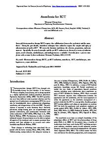
Figure 2.1: The steps taken to execute two dependent arithmetic instructions and their dependencies.
Examples of this trend included IBM’s Power4, which includes two 4-issue processors on a chip instead of a single wider-issue processor, and Intel’s Itanium which relied on VLIW techniques to reduce the amount of analysis and scheduling done at runtime. To give an example of the sort of performance we mean, consider the Alpha 21264 (EV6), which uses two small windows (20 entries for integer and 15 for float) instead of one big window (see [29] for a description of the issue logic in the EV6). The integer window statically assigns each instruction to a group of functional units before enqueueing it. It requires an extra clock cycle for data to move between instructions that happen to have been placed far apart from each other, as compared to if they had been placed near each other. The collective effect is that the EV6 is already paying for its large window size (although the overall cost is apparently acceptable—perhaps 2% on SPEC benchmarks). This chapter outlines the core of a processor that can fetch 8 instructions per clock, issue 20 instructions per clock, and has a window of 128 instructions. This processor, designed in the technology of mid 1999 (0.25µm aluminum), has critical path competitive to processors of the same period (our critical path is under 2ns) and with substantially higher ILP and program speed compared to today’s processors. Our processor relies on a novel design of the wake-up logic and of a multi-unit scheduler [44]. Our designs enable cyclic reuse of the reordering buffer with new instructions continually entering the buffer and taking up the place of the oldest, retiring ones, without having to use circuitry to compress instructions to the beginning of the reordering buffer. We have concentrated on redesigning the processor components that limit the execution time of dependent arithmetic instructions in the reordering buffer. Figure 2.1 shows the steps that must be taken in order to
20
execute two dependent arithmetic instructions without bypassing. In our example, Instruction B depends on the result of Instruction A. Instruction A wakes up Instruction B, once A has been successfully scheduled. Instruction B requests to be scheduled while waiting for the result of A. According to SPICE simulations of our layouts, our wakeup logic runs in 1.34ns and our scheduler logic runs in 1.69ns. Our circuit designs should be viewed as only one stake in the ground. Earlier study of the MIPS R10000 and the Alpha 21264 showed that their circuit implementations of superscalar components would not scale to large buffer sizes [93]. Subsequent processors, such as the AMD K6, have begun to use more scalable implementations to reimplement some of these components. There may well be other, possibly better, designs for the processor components described in this chapter. To our knowledge, there are no such designs in the literature prior to our study, which was published in 2000. While we present new scalable designs for some processor components in this chapter, there are many other processor components that we have not addressed. We have not redesigned the processor’s data paths, only the control paths. We have also not redesigned the logic for bypassing results among numerous functional units. Instead, in our program performance study, we measure a system with no bypasses. Finally, we have not addressed the problems of scaling the memory subsystem. This issue will be addressed in Chapter 3. In our program study, we assume a 32-entry memory buffer that has comparable functionality to the Alpha 21264’s buffer. All of our redesigned superscalar components draw on the same underlying idea. They all exploit the sequential ordering of instructions in a wrap-around reordering buffer and attach one or more cyclic segmented parallel prefix (CSPP) circuits to the reordering buffer. Figure 2.2(a) illustrates an eight-instruction wrap-around reordering buffer. Instructions are stored in the buffer in a wrap-around sequence. The oldest instruction in the buffer is Instruction A, pointed to by the Head pointer. The youngest, most recently fetched, is Instruction H pointed to by the Tail pointer. This work was partly motivated by our research group’s previous theoretical results on asymptotically optimal superscalar processors [48, 72]. In contrast, this work focuses on understanding the engineering problems of the wide-issue processors of the near future.
21
Figure 2.2(a) also shows a linear gate-delay implementation of a CSPP circuit. A CSPP circuit with a linear gate delay consists of a ring of operators,
�
, and MUXes. We attach this ring to the wrap-around
reordering buffer using different associative operators,
�
. The jth entry in the buffer is attached to input
in j , output out j , and segment bit s j of the CSPP circuit. The circuit applies the operator
�
to successive
inputs and assigns the result accumulated so far, also known as a prefix, to each output. The circuit stops accumulating whenever it encounters a high segment bit. For example, if s 6 out2 �
�
1 and s7 �
s0 �
s1 �
0, then
in6 � in7 � in0 � in1 . For the circuit to produce well-defined values, at least one instruction, typically
the oldest, must set its segment bit high in order to stop the cyclic accumulation of inputs. In general, many instructions can raise their segment bits, leading the circuit to accumulate inputs over multiple nonoverlapping, adjacent segments. Although Figure 2.2(a) shows a linear gate-delay implementation of a CSPP circuit; other, logarithmic gate-delay implementations exist. Figure 2.4(a), Figure 2.4(b), Figure 2.5 and Figure 2.6 illustrate four such implementations and we describe them in more detail in Section 2.3. All the CSPP implementations have identical interfaces and functionality, but the logarithmic gate-delay implementations can lead to dramatically faster circuits. The rest of this chapter describes our novel circuits, their VLSI layouts, and simulations, and analyzes the benefits of a large-window processor utilizing these circuits. Section 2.2 describes our designs of the wakeup, schedule, commit, and rename logic in terms of linear gate-delay CSPP circuits. Section 2.3 converts linear gate-delay CSPP circuits to faster, logarithmic gate-delay CSPP circuits and compares several alternative designs. Section 2.4 describes and analyzes our VLSI implementations of wakeup, schedule, and commit logic. Section 2.5 describes our program performance study and analyzes its results. Section 2.6 discusses implications for building a wide-window processor in future technologies.
2.2 CSPP Circuits for Superscalar Components This section shows how different superscalar components can be redesigned using CSPP circuits. Using CSPP circuits, we redesign the commit logic, the wakeup logic, the schedule logic, the rename logic, and the commit logic of a traditional superscalar processor. To simplify our explanation, we show each component
22
redesigned with linear gate-delay CSPP circuits first. In Section 2.3, we will convert our designs to faster logarithmic gate-delay CSPP circuits. Consider, first, the commit logic. The commit logic informs each instruction whether all earlier instructions in the buffer have committed. Figure 2.2(b) shows a linear gate-delay implementation of the commit logic attached to our eight-instruction wrap-around reordering buffer. The commit logic consists of a single one-bit-wide CSPP circuit with the operator AND. The AND gates accumulate the successive answer: “Have all earlier instructions committed?” Each multiplexer passes the accumulated answer to successive instructions, but stops at the oldest one. Figure 2.2(b) includes an example. In the example, wires carrying high signals are displayed in bold; Instructions A, B, E, and F have committed; and the commit logic has informed Instructions B and C that all earlier instructions have committed. Instructions A, B, and C can now act based on the output of the commit logic and their own status. Instructions A and B retire, while Instruction C becomes the new Head Instruction. Our wake-up logic uses CSPP circuits to determine when each instruction’s arguments are ready to be latched off a broadcast bus. Latched arguments remain in the window entry until the entry can be scheduled. The wake-up logic uses one CSPP circuit for each logical register defined in the processor’s instruction set architecture. Each CSPP circuit operates independently of the others and informs the buffer’s instructions about the readiness of its logical register. Figure 2.3(a) shows our wake-up logic for a processor with 32 logical registers. Each instruction in the reordering buffer receives 32 ready bits indicating the readiness of each register. Each instruction then uses a 32-to-1 multiplexer (not shown), for each of its arguments, to select the ready bits corresponding to the registers it needs. Figure 2.3(a) illustrates our linear gate-delay implementation of the wake-up logic for one register, register R5. The figure shows the values passing along the wake-up CSPP circuit. Wires carrying high signals are displayed in bold. The operator
�
for this CSPP circuit is simply a wire that passes the old
value along (i.e., a � b � a). Each instruction in the reordering buffer sets its segment bit high if it writes register R5. It sets its input bit high once it has computed R5’s value. In our figure, Instruction F has already
23
Cyclic Reordering Buffer E:R2=R2+R4
Cyclic Segmented Prefix
Cyclic Reordering Buffer
out0 in0
Commit Logic
E:R2=R2+R4 done
s0 F:R5=R3+R3
out1 in1
F:R5=R3+R3 done
s1 G:R4=R5+R7
out2 in2
G:R4=R5+R7 not done
s2 H:R6=R3+R7 Tail
out3 in3
H:R6=R3+R7 Tail
done
s3 A:R1=R2+R3 Head
out4 in4 s4
B:R8=R9+R9
out5 in5
A:R1=R2+R3 Head Initial Input Set to 1
done B:R8=R9+R9 done
s5 C:R5=R8+R1
out6 in6
All Previous Done
C:R5=R8+R1 not done
s6 D:R1=R5+R1
out7 in7
D:R1=R5+R1 not done
s7 Done? Oldest?
(a)
(b)
Figure 2.2: (a) An 8-entry wrap-around reordering buffer with adjacent, linear gate-delay cyclic segmented parallel prefix (CSPP). The � can be any associative operator, (b) Commit logic using CSPP.
24
Wake−Up Logic
g r rin ffe c rde Bu cli eo Cy R
For R29
Cyclic Reordering Buffer
For R0 R0
E:R2=R2+R4
E:R2=R2+R4
done
done
F:R5=R3+R3
F:R5=R3+R3
done
done
G:R4=R5+R7
G:R4=R5+R7
not done
not done
H:R6=R3+R7 Tail
A:R1=R2+R3 Head
E:R2=R2+R4 3
F:R5=R3+R3 4 request G:R4=R5+R7 4
H:R6=R3+R7 4 Tail
done
done
B:R8=R9+R9
B:R8=R9+R9
done
done
C:R5=R8+R1
C:R5=R8+R1
not done
not done
D:R1=R5+R1
D:R1=R5+R1
not done
not done
Head Instruction Initializes to R5 ready.
request A:R1=R2+R3 4
Head
1
request B:R8=R9+R9 1 request
Done? Writes R5?
(a)
Scheduler Logic
request
A:R1=R2+R3 Head
done
Cyclic Reordering Buffer
H:R6=R3+R7 Tail
done
Wake−Up Logic For R5
C:R5=R8+R1 2
�
4 if request
granted.
R5 ready. D:R1=R5+R1 2 request Requesting? Head?
(b)
(c)
Figure 2.3: (a) An 8-entry wrap-around reordering buffer with adjacent wake-up logic for a processor with 32 logical registers. (b) The wake-up logic for logical register R5. Asserted signals are shown in bold. (c) Scheduler logic scheduling four functional units.
25
computed a value of R5 and set its input bit high; Instruction C has not. As a result, Instruction G is informed that R5 is ready, but Instruction E is not. Our schedule logic uses a single CSPP circuit with addition for its operator
�
. Figure 2.3(c) illustrates
our scheduler which assigns four functional units to the four oldest requesting instructions in a wrap-around reordering buffer. For each buffer entry, the scheduler simply returns the sum, n, of all the older instructions requesting to be scheduled. (The sum can saturate at the number of functional units.) A requesting entry is scheduled to use functional unit n, if the value returned from the scheduler is less than the number of functional units. In the example of Figure 2.3(c), Instructions A,B,D, and E have been scheduled to functional units 0,1,2, and 3 respectively.
2.3 Alternative CSPP Circuits Although, for simplicity, the figures above show linear gate-delay prefix circuits, we found that logarithmic gate-delay implementations can significantly reduce the critical path delay. This section describes and contrasts four different implementations of CSPP circuits that all have only logarithmic gate delay in the window size. The next section will discuss the simulations and the layouts of our superscalar components built from these CSPP circuits. All four CSPP circuits described in this section implement the same function as the circuit of Figure 2.2(a). While the linear gate-delay CSPP circuit in Figure 2.2(a) applied the
�
operator in-order to
successive inputs, the four logarithmic gate-delay CSPP circuits rely on the associativity of the
�
operator,
by applying the operator in parallel to contiguous subsets of the inputs. They all have O � lg n � delays due to gates, but they have varying areas and delays due to wires. The four circuits are: a binary tree, a 4-ary tree, a “thicket” of trees and a “prefix/postfix thicket”. The binary tree circuit is shown Figure 2.4(a). The binary tree consists of a collection of binary tree nodes (each shown with grey backgrounds) that compute a segmented prefix in the way described in [21]. Our circuit is different from the circuit of [21] in that we modified the root node to make the tree implement a cyclic segmented prefix instead of an acyclic segmented prefix [45]. For a reordering buffer with
26
out0 in0 s0
out0 in0
Log−Depth Cyclic Segmented Prefix (CSP)
s0
out1 in1 s1
out1 in1
out2 in2 s2
out2 in2
out3 in3 s3
out3 in3
4−ary tree node
s1
s2
Binary root node
s3
Binary tree nodes
out4 in4 s4
out4 in4
out5 in5 s5
out5 in5
s4
Binary root node.
4−ary tree node
s5
out6 in6 s6
out6 in6
out7 in7 s7
out7 in7
s6
s7
(a) A CSPP circuit made of a binary tree.
(b) A 4-ary tree with a binary root node.
* *
*
(c) 4-ary tree node.
*
*
*
(d) Binary root node.
(e) “Switched operators”.
Figure 2.4: (a) A binary-tree implementation of CSPP. (b) A 4-ary tree with a binary root node. (c) A node in the 4-ary tree. (d) The binary root node. (e) The switched operators used in (c) and (d).
27
n instructions, the gate delay through the binary tree implementation consists of delays3 plus
� �
2 lg n ��� 1 � MUX delays. The delays can be thought of as
���
���
2 lg n � � 1 � �
operator
lg n ��� 1 � operators and MUXes
going up the tree, followed by lg n operators and MUXes going down the tree. A faster version of the tree circuit can be implemented by building a 4-ary tree, as shown in Figure 2.4(b). The details of a 4-ary tree node are shown in Figure 2.4(c–e).The binary root node shown in Figure 2.4(d) is the same one used in Figure 2.4(a). The delays going up the 4-ary tree are the same as the binary tree (although, as we shall see in Section 2.4, using a compound gate to implement a 4-ary MUX can speed up the circuit further.) The delays going down the tree are halved, however. This is because the values going up the tree arrive first and precompute all the values shown in bold. Later, when the value coming down the tree finally arrives, it passes through only one switched operator at the bottom of the 4-ary tree node. Thus the gate delay consists of only 3 2 lg n���
operator delays and 3 2 lg n� MUX delays. The use of 4-ary
trees to implement acyclic prefix is well known (see, for example, the scheduler logic in [93]), but we have not seen any 4-ary trees that implement a cyclic prefix. The 4-ary tree idea can be generalized to other widths. For example, whereas a 4-ary node produces a circuit with a gate delay of 3 2 lg n���
operator and MUX delays, an 8-ary node produces a circuit with
only 4 3 lg n��� operator and MUX delays. The third approach is to build a “thicket” of trees, such as is described in [21, Exercise 29.2-6]. Figure 2.5 illustrates this method. Once again, the main difference between this circuit and the one in the literature is that our circuit implements a cyclic prefix operation. The gate delay through a thicket implementation consists of only lg n � operator and MUX delays. The area increases substantially, however; and the savings in gate delay are partly offset by increased wire delays to traverse that area. One disadvantage of the thicket is that some signals must travel all the way from the bottom of the circuit to the top of the circuit and then all the way back down. Consider, for example, a scenario in which all segment bits are low except for s 6 , the next-to-last window entry. Figure 2.5 highlights one resulting path through the circuit. The value from the last window entry must travel all the way to the top of the circuit in 3 We
write lg n to for the log base 2 of n.
28
the first stage, and then work its way nearly to the bottom of the circuit in the subsequent stages. To address this doubled-wire-length problem in the thicket circuit, Rahul Sami devised what we call a “prefix-postfix thicket”. The prefix-postfix thicket, shown in Figure 2.6, combines the outputs of an acyclic, segmented prefix and an acyclic, segmented postfix in order to generate a CSPP. For example, Figure 2.6 highlights the datapath that computes out 3 , assuming that only one segment bit, s5 , is high. The prefix circuit computes in0 ��� in1 � in2 � . The postfix circuit computes � in5 � in6 � �
in7 . Since the prefix’s segment bit is
low, the root node combines the outputs of the prefix and the postfix circuits, in the correct order, generating the answer: out3 �
� �
in5 � in6 � �
in7 �
���
in0 ��� in1 � in2 �����
As our example illustrates, the “prefix-postfix thicket” computes any output signal while traversing the height of the reordering buffer at most once. The thickets require much more area than do the trees. The tree’s area grows as Θ � n lg n � since the height of the layout is Θ � n � and the width of the layout is Θ � lg n � . (An H-tree layout could get the area of a tree down to Θ � n � , but we are assuming that the window entries are laid out in a linear array for this study.) The thicket’s area grows as Θ � n 2 � for n window entries, since the height of the layout is Θ � n � , and the width of the last stage alone is Θ � n � because n 2 wires must move from the bottom half of the circuit to the top half. The thicket has the advantage, however, that it has half the gate delays of the binary tree. The 4-ary tree is somewhere in between with slightly greater area and about 3 4 the gate delays of the binary tree.
2.4 Implementation and Performance Having enumerated several logarithmic-depth prefix circuits, we will next describe and evaluate our VLSI implementations of wake-up, schedule, commit, and rename logic using each of these circuits and compare the different implementations. To avoid having a very long thin reordering buffer, we assume in our implementations that the reordering buffer is laid out in two columns of 64 buffer entries each (see Figure 2.7.) Each buffer entry is assumed to be 1000λ high. We believe that 1000λ is an overestimate of the height, possibly by more than a factor of 29
out0 in0 s0 out1 in1 s1 out2 in2 s2 out3 in3 s3 out4 in4 s4 out5 in5 s5 out6 in6 s6 out7 in7 s7
Figure 2.5: A CSPP circuit made of a wrap-around “thicket”, with one longest path highlighted.
30
out0 in0 s0
in0 s0 out1
in1 s1
in1 s1 out2
in2 s2
in2 s2 out3
in3 s3
in3 s3 out4
in4 s4
in4 s4 out5
in5 s5
in5 s5 out6
in6 s6
in6 s6 out7
in7 s7
in7 s7
Prefix Thicket
Root Nodes
Postfix Thicket
Figure 2.6: A CSPP circuit made of an acyclic prefix thicket, an acyclic postfix thicket, and root nodes that combine the results from the two acyclic thickets. The wires used by one particular reduction is shown with thick lines.
31
Entry 0
Entry 127
Entry 1
Entry 126
Entry 2
Entry 125
Entry 3
W
W
W
W
Entry 124
1000λ
W
...
W
W
R
Entry 63
W
...
Entry 64
Figure 2.7: The layout of the register window with the 4-ary wakeup logic tree shown.
two. We decided to use a larger-than-necessary buffer height so that our critical-path-length estimate would be too high rather than too low. The various broadcast circuits connecting the window entries to functional units run vertically over the entries, while the commit, wake-up, and schedule circuits run between the two columns of entries. Our circuits’ wire lengths reflect this layout. They include vertical wire lengths to traverse the height of reordering buffer as well as horizontal wire lengths to traverse the other circuits sandwiched between the two columns. Having settled on the buffer’s layout, we then designed our superscalar components from Section 2.2 using each of the CSPP implementations from Section 2.3. We based our designs on a 0.25µm, 5-metal-layer, Aluminum CMOS technology. For each design, we considered a number of alternative implementations, in static, domino and transmission gate logic. We also considered many different sizes for each gate along each
32
2-Tree Delay (ns) Est’d
SPICE
4-tree Area
Delay (ns)
(Mλ2 )
Est’d
SPICE
Thicket Area (Mλ2 )
Est’d
11
Commit
2.06
9
1.82
Wakeup
2.35
900
1.60
1.54
980
770
1.48
1.34
800
24
2.10
(T-gates) Schedule
1.78 2.35
1.94
Delay (ns)
26
Pre/Post Area
Delay (ns)
Area
(Mλ2 )
Est’d
SPICE
(Mλ2 )
1.76
140
1.46
1.41
160
1.99
13000
1.68
1.80
15000
2.03
320
1.64
1.69
360
SPICE
Table 2.1: Circuit delays and areas including step-up and wire costs. Circuits in all the rows, except for the “T-gates” row, use domino logic. Circuits in the “T-gates” row use transmission gates.
circuit’s critical path. We did not consider more than one size ratio for transistors within the same compound gate, however. Different size ratios could perhaps yield circuits faster than the ones we report. We have sized the transistors of our circuits for maximum speed, using a C program that we wrote 4 . Our program assumes that the inputs are minimum-sized and includes any needed step-up inverters. Outputs drive minimum sized gates. The program models the delay of a transistor and of a wire by a piecewisequadratic approximation function that we fitted to match the SPICE simulations of the 0.25µm technology [128]. The program’s input consists of a set of allowed sizes, and a gate-level description of the circuit’s critical path annotated with wire lengths. The program starts out by assigning a random size to each gate, computes the critical path’s delay, and then iterates using a genetic search algorithm to reassign sizes. It takes the program only a few minutes to converge to a very good circuit. We used our estimates to choose the most promising circuits and implement them. We laid out the critical paths of these circuits in Magic, and extracted the circuits using a model which distributes the RC of long wires into a series of resistors and capacitors. We ran SPICE on the circuits, and found that our sizing program’s estimates of the delays are consistently within 10% of the SPICE results. Table 2.1 summarizes, in a table, the results for our best designs. The figure assumes a processor with 32 logical registers and 128-entry wrap-around reordering buffer laid out in two columns. The processor’s wake-up logic includes all 32 CSPP circuits plus a 32-to-1 multiplexer for each argument in the reordering 4 The
program was primarily authored by me and Rahul Sami, with some restructuring by Dana Henry.
33
buffer. The processor’s schedule logic assigns four functional units to the four oldest requesting instructions in the reordering buffer. Each column of the table uses a different CSPP implementation from Section 2.3. Most of the circuits in the table are implemented with domino logic and driving inverters. There are two exceptions. The 32-to-1 MUXes within our wake-up logic are implemented with transmission gates. And the row labeled “T-gates” describes faster implementations of wake-up logic in which all multiplexers are built with transmission gates. The table shows the critical path delay and area estimate for our best commit, wake-up, and schedule designs. For all designs, the table reports the estimated delays generated by our sizing program. The table also includes the delays reported by SPICE for the circuits’ critical paths that we have laid out in Magic and simulated in SPICE. Finally, the table gives an estimate of each component’s area that accounts for both gates and wires. Our area estimates use four metal layers to route signals. Using only four layers likely overestimates area, since existing aluminum technologies already use eight metal layers. Our area estimates may also be somewhat high because we have not optimally sized gates outside of critical paths 5 . The remainder of this section describes our implementations of each logic component in greater detail and analyzes their performance.
2.4.1 Wake-Up Logic The description of the wakeup logic in Section 2.1 presented a simplified view. Our wake-up logic does not only compute the readiness of each argument. It also propagates the number of the functional unit producing each result. A woken-up instruction can use the functional unit number to read its argument off the unit’s result bus. The actual prefix circuit that we simulated thus passes 5-bit values (a ready bit, plus four bits identifying one of sixteen result-generating functional units) through the multiplexers. Thus the circuit is the same as the CSPP circuit described in Figure 2.3, but values traveling through the prefix are 5 bits wide instead of 1 bit wide. Table 2.1 confirms that the wake-up logic is the most area-intensive of our components. Fortunately, one 5 Wire
area dominates gate area, however, limiting the possible overestimate to at most 20–25%.
34
1300λ
24x 10x
18x
6000λ
36x 10x
18x
24000λ
24x 10x
18x 200λ
1x
3x 16x 10x 500λ
500λ
18x
500λ
10x
10x
10x 500λ 10x
10x 22x
1500λ
9x
10x 22x
6000λ
16x
10x 14x
24000λ
18x
10x 10x
200λ
10x 9x 500λ 10x
500λ 10x
500λ 10x
Figure 2.8: The gate sizing and wire lengths for the wakeup logic’s critical path.
of the least area-intensive implementations, the 4-ary tree, is also the fastest. The resulting wake-up logic’s width, for all 32 logical registers, is less than one fourth of the height of the two-column buffer. Using transmission gates, rather than domino logic to implement each multiplexer within the wake-up logic can further speed up the design. We have sized, laid out, and simulated with SPICE the wake-up logic’s critical path, using transmission gates to implement MUXes and trees to implement CSPP’s. Each tree node consists only of transmission-gate multiplexer(s) and driving inverters. The binary tree implementation runs in 1.94ns, whereas the 4-ary tree implementation runs in only 1.34ns according to our SPICE simulation. The 4-ary tree implementation speeds up much more than the binary tree implementation because a 4-ary transmission gate MUX is almost as fast as a 2-ary one, when the select bits are ready in advance. Figure 2.8 shows the critical path through our wake-up logic. The inverters are static. The figure includes the lengths of all wires and the sizes of all gates on the critical path. The gate sizes are given in multiples of the minimum gate width. The transmission gate multiplexers only use N-type transistors. The root is located on the far right of Figure 2.8 and uses a two-to-one multiplexer. SPICE simulation of our wake-up logic 35
yields worst-case delay of 1.34 ns, whereas our sizing program predicted 1.48 ns. There is one instance of the wakeup logic for each logical register. The final 32-to-1 multiplexer chooses one of the wakeup signals depending on the instruction’s operand field.
2.4.2 Scheduler Logic Our scheduler schedules four functional units as illustrated in Figure 2.3. All 128 reordering buffer entries can request a unit. The four oldest requesters receive positive acknowledgements together with the number of the unit that has been assigned to them. The rest receive a negative acknowledgement. Not surprisingly, the scheduler is our slowest component. To minimize delay, we have laid out the critical path of our scheduler using a prefix/postfix thicket implementation of CSPP and a unary encoding of each sum propagating through the thicket. Figure 2.9 shows the critical path through our scheduler. The ai signals encode the unary sum of the left sub-tree, and the b i signals encode the unary sum of the right sub-tree. Each box represents one compound domino logic gate. The inverters are static. SPICE simulations of our critical path yielded worst-case delay of 1.69ns, whereas our sizing program predicted 1.64 ns. In our study of instruction-level-parallelism, we use five separate schedulers to schedule four integer ALUs, four branch units, four memory units, four integer multiply units, and four floating point units. The five schedulers implemented with prefix/postfix thickets, require more total area than our wake-up logic implemented with a 4-ary tree. Together, the five schedulers’ width is less than half of the height of the the two-column reordering buffer. We account for this width when computing the wire delays of all of our circuits. Our scheduler’s speed compares favorably to the one described by Palacharla [93]. Palacharla used a synthetic 0.35µm and 0.18µm process extrapolated from 0.8µm and 0.5µm technologies. We used 0.25µm process parameters from MOSIS. Palacharla did not account for wire delays, whereas we did. We used a linear interpolation of the delay between the 0.35µm and 0.18µm to conclude that Palacharla predicts scheduler delays of about 0.8ns for a window of 128. In comparison our scheduler circuit for one functional unit has a delay of 0.71ns if we assume that all wires are of length 0. If we include wire delays for windows
36
5000λ 1000λ 1x
3x
500λ
8x f1
2000λ 14x
40x f1
4000λ 40x
40x f1
8000λ 28x
40x f1
16000λ 40x
40x f1
32000λ 40x
40x f1
500λ 40x
28x f1
500λ 22x
8x f1
6x
40x
22x
28x
14x
24x
18x
9x
f2
f2
f2
f2
f2
f2
f2
f2
28x
26x
20x
10x
24x
12x
9x
f3
f3
f3
f3
f3
f3
f3
22x
9x
20x
14x
18x
10x
10x
f4
f4
f4
f4
f4
f4
f4
40x
40x
40x
40x
40x
8x f1
500λ
f1
500λ
f1
500λ
500λ
f1
f1
500λ
40x
f1 ��� ���
a1 � S � b1
f1
f2 ��� ���
a1 � b1 � S � a2 � S � b2
f3 ��� ���
a1 � b2 � S � a2 � b1 � S
6x
40x
22x
28x
14x
24x
f2
f2
f2
f2
f2
f2
28x
26x
20x
10x
24x
f3
f3
f3
f3
f3
22x
9x
20x
14x
18x
f4
f4
f4
f4
f4
� a3 � S � b3 f4 ��� ���
a1 � b3 � S � a2 � b2 � S
� a3 � b1 � S � a4 � S � b4
Figure 2.9: The gate sizing and wire lengths for the scheduler’s critical path.
that are 100λ high, then our circuit incurs a delay of 0.88ns, and for windows that are 1000λ high, then the circuit delay is 1.32ns. Palacharla shows how to schedule two functional units of the same type (e.g., two FP adders), by chaining two schedulers together, which would give a delay of 2.64ns using 1000λ windows. Our scheduler for twice as many functional units (four instead of two) with windows of 1000λ has a delay of only 1.69ns.
2.4.3 Commit Logic We have laid out the critical path through a prefix/postfix thicket which computes the commit bits within 1.41ns. The gate sizing and wire lengths are shown in Figure 2.10. The A signals are from the left subtree, the B signals are from the right subtree, and the S’s are the segment signals. Since the commit CSPP is only one bit wide, the VLSI area of the prefix/postfix thicket is negligible.
37
5000λ 3x
40x
A
�
B
�
�
24x
S
B
40x
S
A
�
AS
�
AS
AS
�
B
B
B
B
500λ
500λ
28x
�
A
20x
�
B
40x
B S
�
500λ
A
�
40x
�
500λ
B
40x
B S
A
18x
�
B
B
40x
�
500λ
A
�
40x
�
32000λ
AS
�
28x
�
AS
A
B
AS
B
500λ
16000λ
S
A
�
40x
�
40x
�
A
�
B
B
500λ
40x
S
AS
A
�
40x
�
A
A
B
S
AS
B
�
40x
B
3x
�
AS
AS
�
8000λ
B
12x
B S
�
�
40x
�
B
3x
A
B
B
1x
4000λ
AS
�
40x
�
AS
A
AS
2000λ
AS
�
AS
A
AS
1000λ
500λ
B
B
B
B
B
B
B
S
S
S
S
S
S
S
Figure 2.10: The gate sizing and wire lengths for the commit logic’s critical path.
2.4.4 Rename Logic If each instruction in our instruction-set architecture generates only one result, we could implement rename logic in much the same way as our wake-up logic. We would pass through each logical register’s CSPP a 7-bit address instead of a 4-bit functional-unit number and a ready bit. The rename logic supplies each entry in the entire buffer with the the physical register numbers of its arguments. The physical register numbers in this implementation are the reordering buffer addresses of the instructions that write them.
2.5 Performance Impact The preceding sections show a strategy for redesigning many of the superscalar components to operate on a large wrap-around reordering buffer. Our circuits implement a reordering buffer that is more than three times larger than the reordering buffers of commercial processors (from 1999-2000), while reaching comparable clock speeds in a comparable technology. Program performance does not just depend on clock speeds, however, but also on the instruction-level parallelism (ILP) uncovered by the processor. In this section, we will try to quantify the effect that larger reordering buffers might have on the ILP of next-generation processors.
38
2.5.1 Our Simulation Environment We based our studies of ILP on the SIMOS instruction-level simulator of the Alpha Instruction Set Architecture [102, 125]. To measure instruction-level parallelism, Bradley Kuszmaul and I added a time-stamping mechanism to the SIMOS in-order simulator. The time-stamping mechanism is described in greater detail in Chapter 5. We attach a time-stamp to each architected register. For example, when simulating an instruction “R1:=R20+R23”, we set the time-stamp of R1 to one plus the maximum of the time-stamps of R20 and R23. The program counter also has a time-stamp, so when executing “BRANCH-IF-ZERO R3 +5”, which branches forward 5 instructions if R3 is zero, we can “max-in” the time-stamp of R3 to the stamp of the program counter. When executing a memory instruction, we can, for example, keep a single time-stamp on the memory system, which effectively serializes all store instructions, and makes every load instruction depend on the most recent store instruction (even if that store was to a different location). These simulation rules would compute the critical path for a processor with an infinite window, and an infinite number of functional units, no memory parallelism, and no branch speculation. It turns out that we can modify the time-stamping rules to handle many more interesting variations. We implemented time-stamping rules that model the delays induced by a limited fetch width from an infinite instruction cache or trace cache [104, 33] with a hybrid branch predictor [84] and misprediction penalties, by a limited window size with three different window refilling policies (wrap-around, compressing, and flushing), by a limited number of specialized, pipelined functional units assigned to oldest requesting instructions, and by an out-of-order load/store unit [65]. By maintaining multiple time-stamps for each state and resource, we can simulate a number of different processors concurrently in one simulation run. We have also not found an efficient way to model the effect of a limited number of functional units and a wraparound window in which the next instruction scheduled is the ready instruction in the lowestnumbered window entry, i.e. when the window is wrap-around but the scheduler is not. We believe that 39
several existing processors use such a scheduler. Such a scheduler is likely to be worse than a pure wraparound scheduler: it is usually preferable to schedule an older instruction over a younger instruction so that it can be retired sooner. One problem with a non-wrap-around scheduler on a wrap-around window is that it can exhibit non-monotonic behavior. 6 It can be very difficult to write good compilers for processors that exhibit non-monotonic behavior. The earliest time-stamping processor simulator that we know of was implemented for the GITA taggedtoken dataflow architecture [90]. We are also aware of a time-stamping simulation developed independently by Intel for the Pentium Pro processor. See Chapter 5 for a more detailed description, and a validation of our time-stamping algorithm.
2.5.2 The Simulated Processors We simulated two different processors using our time-stamping simulator. Both processors implement the 21264’s instruction set. The first processor, called α, resembles commercial processors of late 1990’s and provides a baseline for our study. The α has a 4-instruction fetch width and a single 32-instruction reordering buffer shared by all instructions. The processor fetches an unaligned block of four statically adjacent instructions at a time. The α can issue up to nine instructions at a time. The functional units, their numbers, and their latencies are described in Table 2.2. The second processor that we simulated, called β, approximates a processor that we believe could be built using our redesigned superscalar components and other recent advances. The β processor wakes up, schedules, and issues instructions from a single 128-instructions reordering buffer. Using a trace cache [104, 33], the processor fetches an unaligned dynamic sequence of eight instructions at a time. As a result, fetching of instructions only incurs delays when a mispredicted branch is encountered, rather than on every branch. The β can issue up to twenty instructions at a time. The functional units, their numbers, and their latencies are also described in Table 2.2. The two processors, α and β, share a number of characteristics. Both processors use a hybrid branch 6A
non-monotonicity in a processor is a situation where adding an instruction to the inner loop of a program can speed up the
program [69].
40
Common Characteristics:
Hybrid Branch Predictor (see [84]) Predictor selection 4096 2-bit counters (1024KB) Local Predictor 4096 2-bit counters (1024KB) Global Predictor (gshare w/ 3 bits) 8192 2-bit counters (2048KB) 32 Entry jump prediction stack 32 Entry load/store unit Instruction Latencies:
α
Integer ALU (non-multiplication)
1 (2) Cycles
Integer Multiply
7
Branch
1 (2)
Memory
3
Floating Point (non-division)
4
FP Single Precision Division
12
FP Double Precision Division
15
β
32 Entry Window
128 Entry Window
4-wide fetch
8-wide fetch
Fetch until taken branch (except for gcc T )
Fetch until mispredicted branch (except for gcc I )
2 integer ALUs
4 integer ALUs
2 branch units
4 branch units
2 memory ports
4 memory ports
1 integer multiplier
4 integer multiplier
2 floating point units
4 floating point units
Table 2.2: Simulated processor parameters
41
predictor that dynamically chooses between two branch predictors and incurs a 3-cycle penalty on a branch misprediction [84]. The branch predictor tables are the same size for both processors. (It may be that a larger branch predictor would make sense for a larger processor.) Both also have fully pipelined functional units and infinite-size caches. The two processors differ in two important aspects: the structure of their reordering buffer and the use of bypasses. The α processor uses a compressing reordering buffer much like the 21264, while the β uses a wrap-around reordering buffer. A compressing reordering buffer can make better use of its entries. On every clock cycle, the α’s compressing buffer retires all instructions that have finished executing and compresses all remaining entries by pushing them up to the top of the buffer. Thus, on every clock cycle, all unused entries are ready to be refilled with new instructions. In contrast, a wrap-around buffer cannot refill an unused entry until all older instructions have finished. All the circuits described in this chapter can operate on a compressing buffer just as well as a wrap-around one 7 ; however, we do not know how to compress a 128-instruction reordering buffer quickly. For this reason, the β assumes only a wrap-around buffer. Unlike the α, the β also suffers from lack of bypassing. In today’s processors, bypass paths allow many dependent instructions to issue back to back. With twenty functional units, we assume that the α will require an additional clock cycle between certain types of dependent instructions. We assume that instructions with multiple-cycle execution latencies can overlap their execution with the precharging of their results’ paths, allowing dependent instructions to issue without delay. Instructions with one-cycle execution latencies cannot precharge their results’ paths, however, because their dependents have not yet been scheduled. As a result, one-cycle instructions effectively cost a two-cycle delay.
2.5.3 Our Simulation Results We ran a number of simulations in order to better understand the performance of the α and the β and the performance loss associated with the use of a wrap-around buffer and the lack of bypassing. Table 2.3 and Table 2.4 shows the results of our simulations. The figure shows the average instruction7 In
fact, the schedule and commit logic can be made to run faster on a compressing buffer by eliminating segment bits.
42
Minimum Latency = 1
Minimum Latency = 2
EV6/700
α (4-fetch) (int)
(fp)
Wrap
Compress
Flush
Wrap
Compress
Flush
IPC
go
2.20
2.22
1.89
1.96
2.05
1.59
1.03
gcc
2.40
2.45
2.09
2.13
2.24
1.75
2.13
compress
1.64
1.68
1.33
1.54
1.68
1.12
1.37
li
2.62
2.67
2.21
2.44
2.49
1.97
1.27
ijpeg
2.63
2.70
2.30
2.39
2.64
1.79
2.75
perl
2.54
2.86
2.00
2.18
2.52
1.71
1.11
vortex
3.11
3.14
2.53
2.87
3.11
2.25
1.99
tomcatv
2.50
2.53
2.21
2.09
2.16
1.76
1.29
swim
3.52
3.97
2.37
3.52
3.97
2.37
0.99
su2cor
2.45
2.53
2.14
2.01
2.13
1.70
0.80
hydro2d
2.59
3.43
1.72
2.58
3.43
1.71
1.38
mgrid
3.34
3.55
2.18
3.33
3.54
2.17
2.10
applu
2.52
3.20
1.71
2.49
3.17
1.68
0.86
turb3d
3.46
3.54
2.64
3.42
3.53
2.54
1.78
apsi
2.46
3.12
1.76
2.44
3.10
1.74
1.23
fpppp
2.56
3.12
1.76
2.55
3.10
1.74
2.04
wave5
2.68
3.42
1.91
2.59
3.32
1.82
1.11
All benchmarks warmed up for 512M
(229 )
instructions, and then measured over the next 512M
instructions. Table 2.3: Simulated IPC for the α processor and its variations.
43
level parallelism of the SPEC cpu95 benchmarks [119] as measured by our time-stamping simulator. The benchmarks were compiled by and for an Alpha 21164 processor using the Digital C compiler invoked with cc -migrate -std1 -O5 -ifo -om
which is the standard vendor-supplied compiler option for compiling SPEC95. Since the 21164 is an inorder processor, our code was not optimized for the out-of-order features of the 21264. The highlighted columns in the figures correspond to the two described processors, α and β. Despite its limitations, the 128buffer β substantially outperforms the 32-buffer α. Even on benchmarks such as gcc which have relatively little parallelism, the wide-window processor shows a significant performance gain. The remaining columns vary the structure of the reordering buffer and the bypassing policy. The columns labeled “Wrap” and “Compress” report the performance of a wrap-around reordering buffer and a compressing reordering buffer, respectively. The columns labeled “Flush” are a strawman architecture in which when the window fills up, all instructions must retire before the next instruction can run. We found that the compressing window only buys a small amount of additional performance, and the flushing window is much slower. The columns labeled “Minimum Latency = 2” force all instructions to have at least a latency of two clock cycle in order to model the lack of bypassing in the β processor. Increasing the latency of the integer unit to two incurs a fairly significant overhead, but does not outweigh the benefit of a large reordering buffer. For comparison, we also report in the right-most column the average instruction-level parallelism achieved by a real machine, an Alpha GS140 21264 700MHz EV6 (the rightmost column.) We have derived these numbers by measuring the number of instructions executed for each SPEC benchmark and dividing by the clock speed and by the published runtimes. This IPC is only an estimate, since the published CPU95 results for the 21264 are compiled with a newer compiler, and so the instruction counts are different. This IPC should should resemble the IPC of our α processor. Comparing the α to the EV6, we conclude that our simulation can reasonably model the performance of some benchmarks (gcc, compress, ijpeg), but predicts a much higher IPC for other benchmarks (go, swim, su2cor) than is actually achieved by a 21264. We expect that many variables contribute to the inaccuracy.
44
First, the two processors differ in a number of significant ways. The 21264 has an integer window of 20 instructions and an FP window of 15 instructions, with a clustering mechanism that can further increase latencies. The α, on the other hand, has one window of 32 instructions. For example, [104] showed that the performance of the go program is very sensitive to window size even when holding everything else constant, and thus our 32-entry window may be better than the 21264’s split 40-entry window. The IPC numbers in [104] match ours fairly closely for go. The α also has two general FPU’s instead of one FP adder and one FP multiplier, two general-purpose memory ports instead of one for each window, and a pipelined divider. In addition, the α fails to model cache misses including I/O traffic. To isolate the impact of the trace cache on the performance, we also ran the gcc SPEC benchmark on the small processor with a trace cache, and on the big processor with the non-trace I-cache. Table 2.5 shows the impact of the trace cache. Surprisingly, the trace cache is responsible for a relatively small part of the speedup.
2.6 Conclusion By using the optimized circuits presented in this chapter, we conclude that superscalar processors with large instruction windows can be build. Architectural ideas such as clustering [93], SMT [121], and trace caches [104, 33] are largely orthogonal to our results. For example, processors should still be clustered, but the size of the windows can be made much larger. Patt et al [96] have been arguing for several years that the best use of a chip with a billion transistors is to build a single large uniprocessor. Our results suggest that such a processor can and should be built. In this chapter, the effects of accessing caches has largely been ignored. As the size of a superscalar processor’s execution core increases, the time required to access even the first level caches increases. Clustering enables a large instruction window to be clocked at very high clock speeds, but does nothing to reduce cache latency. In fact, a very large core may require an entire cycle just for a load instruction to get to the first level cache before the cache access can even start. The next chapter addresses the problem of long cache latencies in large superscalar processors.
45
Minimum Latency = 1
Minimum Latency = 2
EV6/700
β (8-fetch) (int)
(fp)
Wrap
Compress
Flush
Wrap
Compress
Flush
go
3.11
3.11
2.79
2.72
2.73
2.36
—
gcc
3.32
3.33
3.05
2.85
2.87
2.55
—
compress
2.01
2.01
1.84
1.99
1.99
1.68
—
li
3.33
3.33
3.11
3.04
3.04
2.82
—
ijpeg
4.82
4.91
4.27
4.50
4.64
3.46
—
perl
3.23
3.23
2.92
2.75
2.75
2.46
—
vortex
4.61
4.61
4.12
4.31
4.33
3.73
—
tomcatv
3.24
3.24
3.05
2.59
2.59
2.38
—
swim
6.31
6.36
4.16
6.30
6.36
4.15
—
su2cor
3.10
3.10
2.91
2.46
2.46
2.25
—
hydro2d
5.34
5.56
3.73
5.22
5.42
3.66
—
mgrid
5.88
5.89
4.20
5.84
5.87
4.16
—
applu
4.67
5.03
3.24
4.59
4.99
3.13
—
turb3d
6.65
6.70
5.19
6.35
6.43
4.86
—
apsi
4.66
4.77
3.34
4.56
4.70
3.25
—
fpppp
3.75
3.83
2.85
3.73
3.81
2.83
—
wave5
4.96
5.14
3.52
4.73
4.89
3.36
—
All benchmarks warmed up for 512M
(229 )
instructions, and then measured over the next 512M
instructions. Table 2.4: Simulated IPC for the β processor and its variations.
46
Minimum Latency = 1
Minimum Latency = 2
GS140, 6/700
α
Wrap
Compress
Flush
Wrap
Compress
Flush
Spec Base
gccI
2.40
2.45
2.09
2.13
2.24
1.75
2.13
gccT
2.49
2.58
2.11
2.18
2.34
1.76
—
gccI
3.14
3.14
2.95
2.74
2.74
2.49
—
gccT
3.32
3.33
3.05
2.85
2.87
2.55
—
β
All benchmarks warmed up for 512M (229 ) instructions, and then measured over the next 512M instructions. Table 2.5: The impact of the trace cache. The runs labelled gcc I used a traditional I-cache, where the runs labelled gccT used a trace cache model.
47
Chapter 3
Speculative Clustered Caches1 In the previous chapter, we showed how to construct fast circuits for implementing the instruction windows of superscalar processors. In this chapter, we discuss and address the problem of increased memory latencies as the size of the processor increases. In the following chapters, we deal with the problems of branch prediction and efficiently evaluating superscalar processor designs. Although our circuits are fast, further increasing the size of the reorder buffer still results in an overall decrease in clock speed. To enable larger instruction windows and faster clock speeds, clustering is needed. Clustering partitions the instruction window and functional units into smaller groups, or clusters, each of which may be clocked at much faster rates. The processor must forward the results from one cluster to other clusters where consuming instruction may need the data. Past researchers have designed such microarchitectures, but primarily from the perspective of analyzing the performance impact of the additional delays due to inter-cluster bypassing. In this chapter, I report on my joint work with Dana Henry, Rahul Sami and Bradley Kuszmaul in addressing the performance of the cache hierarchy in large, clustered superscalar processors. As either the size of individual clusters or the total number of clusters increases, the physical distance to the first level data cache increases as well. Although clustering may expose more parallelism by allowing a greater number of instructions to be simultaneously analyzed and issued, the gains may be obliterated if the latencies to 1 This
work is joint work with Dana S. Henry, Bradley C. Kuszmaul and Rahul Sami and parts were reported in [49].
48
memory grow too large. We propose to augment each cluster with a small, fast, simple Level Zero (L0) data cache that is accessed in parallel with a traditional L1 data cache. The difference between our solution and other proposed caching techniques for clustered processors is that we do not support versioning or coherence. This may occasionally result in a load instruction that reads a stale value from the L0 cache, but the common case is a low latency hit in the L0 cache. We first design a 8-cluster processor and analyze the impact of the L0 cache on this specific processor configuration. We then simulate a wide range of processor configurations to demonstrate the effectiveness of the L0 cache for different numbers of clusters, cluster sizes, inter-cluster register bypassing networks and instruction-to-cluster distribution policies. Our simulation studies show that 4KB, 2-way set associative L0 caches provide a 6.5-12.3% IPC improvement over the range of simulated processor configurations.
3.1 Introduction The trend in modern superscalar uniprocessors is toward microarchitectures that extract more instruction level parallelism (ILP) at faster clock rates. To increase ILP, the processor execution cores use multiple functional units, buffers, and logic for dependency analysis to support a large number of instructions in various stages of execution. Such a large window of execution requires very large and complex circuits in traditional superscalar designs. Techniques such as very deep pipelining, clustering, and using fast circuits such as those described in Chapter 2 can help maintain aggressive clock speeds, but fail to address a crucial component of the performance equation: cache latency. As the processor core increases in size, and the clock cycle time decreases, the number of cycles required to load a value from the cache continues to grow. In Figure 3.1, we show the harmonic mean IPC performance across the SPEC2000 integer benchmarks for a one-cluster processor (left most bar) and for several configurations of an eight-cluster processor. Due to the additional area of the eight-cluster processor, we are forced to increase the latency to the level-one data cache. The second bar in Figure 3.1 shows the performance of the 8-cluster processor with a larger 6-cycle L1 latency to compensate for the signal propagation delays across the extra chip area. The third bar shows the unrealistic case where we do not adjust the
49
L1 latency for the increased area of the eight-cluster processor. In this chapter, we present our speculative, clustered Level Zero (L0) data caches, an effective, yet simple technique to address the cache latency problem in clustered superscalar processors. As shown in Figure 3.1, augmenting the eight-cluster processor with L0 caches (rightmost bar) provides a 26.7% IPC increase over the single cluster configuration, versus only a 16.3% increase for the configuration without L0 caches. Our caching solution achieves an IPC rate that is within 2% of the unimplementable configuration with the 3-cycle L1 cache. The increasing size of the processor core forces the L1 data cache to be placed further away, resulting in longer cache access latencies. Larger on-chip caches further exacerbate the problem by requiring more area (longer wire delays) and decode and selection logic. Modern processors are already implementing clustered microarchitectures where the execution resources are partitioned to maintain high clock speeds. Two-cluster processors have been commercially implemented [35, 65], and designs with larger numbers of clusters have also been studied [7, 98]. We propose to augment each cluster with a small Level Zero data cache. The primary design goal is to maintain hardware simplicity to avoid impacting the processor cycle time, while servicing some fraction of the memory load requests with low latency. To avoid the complexity of maintaining coherence or versioning between the clusters’ L0 caches, a load from a L0 cache may return erroneous values. The mechanisms that already exist in superscalar processors to detect memory-ordering violations of speculatively issued load and store instructions can be used for recovery when the L0 data cache provides an incorrect value. The chapter is organized as follows. In Section 3.2, we briefly review related research in clustering processors and caching in processors with distributed execution resources. Section 3.3 details the base processor configuration used in our simulation studies, and also explains the simulation methodology. Section 3.4 describes our speculative L0 cache organization, the behavior of the caching protocol, and analyzes the performance for the base processor configuration. Section 3.5 presents our performance results over a wide range of processor and L0 cache configurations. Finally, Section 3.6 concludes the chapter.
50
2 1 cluster (3 cycle) 8 cluster (6 cycle) 8 cluster (3 cycle) 8 cluster + L0 cache
1.8 1.6
Harmonic Mean IPC
1.4 1.2 1 0.8 0.6 0.4 0.2 0 Figure 3.1: The performance impact of increasing level-one data cache latency due to a large processor core. The L0 cache helps reduce the effects of the large L1 cache latency.
51
3.2 Related Work Clustering breaks up a large superscalar into several smaller components [28, 64, 104, 114]. To the degree that most register results travel only locally within their cluster, the average register communication delay is reduced. At the same time, smaller hardware structures associated with each cluster run faster. There has been much research in clustered microarchitectures. Palacharla et al. studied the critical latencies of circuits in superscalar processors and showed that the circuits do not scale well [93]. They suggested dividing the processor core into two clusters to address the complexity of more traditional organizations. In Chapter 2, we showed how to design more scalable circuits for superscalar processors. Nevertheless, clustering is still an attractive technique to attain even faster clock rates. Our circuits may simply allow the individual clusters to be larger. The Alpha 21264 implemented a two-cluster microarchitecture [35, 65]. For highly-clustered processors, the manner in which instructions are assigned to clusters may play an important role in determining overall performance. Baniasadi and Moshovos explored different instruction-distribution heuristics for a quad-clustered superscalar processor with unit inter-cluster register-bypassing delays [7]. In many of these studies, the focus is on the communication of register values between clusters and how this additional delay affects overall performance. Therefore to isolate these effects, the assumptions about the cache hierarchy are a little relaxed. Although the cache configurations (size and associativity) used in these studies are reasonable (32KB to 64KB, 2- or 4-way set associative), the cache access latencies of one cycle [93, 98] and two cycles [7] are unrealistically fast. Even in our study in Chapter 2, we used very optimistic assumptions about the cache to measure the potential impact of a large instruction window. The aggressive clock speeds of modern processors force the computer architect to choose either smaller and faster caches (for example the 2 cycle, 8KB, 4-way L1 cache on the Pentium 4 [54]) or larger and slower caches (for example the 3 cycle, 64KB, 2-way L1 cache on the AMD Athlon [86]). In either case, the average number of clock cycles needed to service a load instruction is likely to increase due to increased miss rates or longer latencies. In this chapter, we examine the performance implications of considering more realistic cache access latencies in the context of large, clustered superscalar processors. For clustered superscalars with in-order instruction distribution, Gopal et al. [38] propose the Specu-
52
lative Versioning Cache to handle outstanding stores. In their approach, small per-cluster caches, which we will refer to as level zero or L0 caches, and the L1 run a modified write-back coherence protocol. The modifications allow different caches to cache different data for the same address. A chain of pointers link different versions of a memory address. A cluster that issues a load from an uncached address initiates a read request along a snooping bus. The responses from all clusters’ L0’s and the global L1 are combined by a global logic, the Version Control Logic, and the latest version is returned. Similarly a cluster’s first store to a given address travels across the snooping bus and invokes the global logic that inserts the store into the chain of pointers and invalidates any mispredicted loads between that store and its successor in the chain. Both operations require that data travel back and forth across all the clusters and to L1. Hammond et al. [41] proposed a similar solution for the Hydra single-chip multiprocessor.
3.3 Base Processor Configuration and Simulation Environment We start by briefly describing our processor parameters and our simulation environment. We have chosen a simple integer processor cluster that we believe can be clocked at an aggressive clock speed. We loosely model a single integer cluster of our processor on the Alpha 21264 [35, 65] integer core. The processor executes the Alpha AXP instruction set and uses resources summarized in Table 3.1. Each cluster’s area approximates that of the 21264 integer core scaled down to a 0.18µm copper process. For single-cluster configurations, we model a wrap-around instruction window. For multiple-cluster configurations, we also retire instructions in program order, but only reuse a cluster after all instructions in that cluster have retired. Figure 3.2 shows the floorplan for our clustered processor. Table 3.1 also describes the parameters of our initial instruction and data memory hierarchies, without any clustered L0 data caches. For our Level 1 memory system, we use a banked L1 cache and a banked load store unit (Load Store Unit), similar to the interleaved ARB [32]. We propose using 16 banks, with each bank containing 8KB of cache and a 16-entry Load Store Unit, and a pipelined butterfly network connecting the clusters with Level 1. When an Load Store Unit bank is full, only the oldest memory instruction can
53
Instruction Fetch
0.38cm
(40KB Trace Cache & 16KB Instruction Cache)
1.89cm
Cluster 0
Cluster 1
Cluster 2
Cluster 3
(20 instrs.)
(20 instrs.)
(20 instrs.)
(20 instrs.)
Cluster 7
Cluster 6
Cluster 5
Cluster 4
(20 instrs.)
(20 instrs.)
(20 instrs.)
(20 instrs.)
0.34cm
0.34cm
L1 Network
0.15cm
Global LSU and L1 Data Cache (128KB)
0.68cm
1.38cm
Figure 3.2: Processor floorplan
54
Number of Clusters Cluster Window Size Cluster Issue Width Cluster Functional Units
Cluster Interconnect Instruction Distribution L1 D-Cache
Data TLB Load Store Unit L1 I-Cache Instruction TLB Unified L2 Cache Trace Cache [33, 103] Main Memory Branch Prediction Decode/Rename Bandwidth Instruction Fetch Queue Load Misspeculation Recovery
8 20 instructions per cluster 4 instructions per cluster 4 Integer ALUs 1 Integer Multiplier 2 Memory Ports Unidirectional Ring 1 cycle per cluster Sequential 64KB, 4-way set associative 6 cycle latency 16 banks 128 entries, 4-way set associative 30 cycle miss latency 16 entries per L1 bank 5 cycle latency 64KB, 2-way set associative 6 cycle latency 64 entries, 4-way set associative 30 cycle miss latency 2MB, 4-way set associative 15 cycle latency 512 traces 20 instruction per trace 76 cycle latency 33KB McFarling (gshare/local) [84] 10 instructions per cycle 32 instructions Selective Re-execution
Table 3.1: The 8-cluster processor configuration
55
issue to that bank. We do not simulate contention in the banks or the network; however, our studies 2 indicate that with 16 banks, contention in the butterfly or at the banks does not significantly affect performance. The processor aggressively speculates on loads, issuing them as soon as their arguments are ready even if there are earlier unresolved stores. We use the selective re-execution method of recovering from misspeculated loads [103]. One cycle after a load instruction is informed that it has mispredicted, it rebroadcasts its result causing any chain of dependent instructions to iteratively reissue. The mispredicted load’s immediate children must first request to be scheduled before reissuing. Unlike most other instructions, they cannot overlap their scheduling stage with the rebroadcasting of their parent load instruction’s value. If the dependencies are across clusters, we charge additional cycles corresponding to the interconnect delay. We base our studies of ILP on the cycle-level out-of-order simulator from the SimpleScalar 3.0 Alpha AXP toolset [4, 11]. We added support for modeling an instruction window partitioned into multiple clusters. We model inter-cluster delays that correspond to a unidirectional ring interconnect. We simulated the SPEC2000 integer benchmarks [119]. The benchmarks were compiled on a 21264 with full optimizations. We used the train data set for all simulations. The simulation windows were chosen to skip the initial warmup code of the benchmarks. We simulated each benchmark for 50 million instructions. Throughout this section, the mean IPC refers to the geometric mean of the IPC across all benchmarks.
3.4 The Clustered Cache This section adds our new memory hierarchy to our clustered processor. We first present an abstract view of our clustered L0 caches, and describe the behavior of loads and stores in our clustered processor. We then present the details of our implementation along with a performance analysis. We also explore other points in the design space by considering different L0 cache configurations and store broadcasting behaviors. 2 We
observed the number of memory requests destined for the same bank on the same cycle, and found the number of such
conflicts to be small.
56
Store Communication Mechanism Cluster1 stores
remote stores Cluster2 stores
Cluster1 L01
remote stores
remote stores Clustern stores
Cluster2
Clustern
L02
L0n
L1 Data Cache and LSU
Figure 3.3: An n-cluster processor with independent L0 caches
3.4.1 The L0 Protocol In designing the cache model, we stress the importance of hardware simplicity, requiring minimal changes to existing structures, so as not to impact the cycle time. Our model is illustrated in Figure 3.3. Each Clusteri has its own private (local) cache L0 i , in addition to a global shared L1 cache. The L0 caches
contain only values generated by retired instructions; this eliminates the extra hardware required to support multiple versions of a value. We also require that values loaded from the L0 caches are always treated as speculative values, which must be verified later. This requirement greatly simplifies the design, because it obviates the need for a coherence mechanism between the multiple L0 caches and the L1 cache. Thus, the L0 caches are truly local structures, which do not require any new global structures for correct execution. To improve the performance of these L0 caches, we allow for a Store Communication Mechanism to communicate stores from their source cluster to other clusters, as shown in Figure 3.3. Again, our model does not require that all stores are sent to all clusters: any particular store may be received by none, some, or all of the other clusters. This is a scalable solution, and enables the design of simple hardware for the common case, without worrying about correctness in rare corner cases. In addition to L0 data caches, the memory hierarchy includes a global load store unit, and the L1 data cache. The global Load Store Unit and L1 data cache are collectively referred to as Level 1. When a memory
57
instruction is sent to the Load Store Unit, the instruction’s location in the window is included so the Load Store Unit can identify the correct order of the instructions. All loads and stores behave according to the following protocol. The configuration without L0 caches can be treated as a special case in which the L0 caches have zero size.
Load Issue: A load is issued when its address is ready, and the load has been scheduled to a memory port. The L0 data cache in the load’s cluster is accessed. If the load hits in the L0 cache, the value is returned in a single cycle. Whether or not the L0 cache hits, the load is simultaneously issued to Level 1. The load arrives at the Load Store Unit sometime later. The Load Store Unit is then scanned for an earlier store to the same address. If such a store is found, the value is sent back to the load’s cluster. If such a store is not found, the data is retrieved from the L1 data cache or higher levels of the memory hierarchy, and sent back to the cluster. If the load hit in the L0 cache, then when the load’s data arrives from Level 1, the value is compared against the previously used L0 value. If they differ, a load misspeculation is flagged.
Store Issue: A store is issued when its address and data are ready, and the store has been scheduled to a memory port. The address and data are sent to the Load Store Unit. Upon arrival at the Load Store Unit, the address is compared against newer loads that have already reached the Load Store Unit. The search is truncated if a newer store to the same address is encountered. If a conflicting load is found, a load misspeculation is flagged and the store’s value is forwarded to the dependent load’s cluster. An issuing store may also be sent through the Store Communication Mechanism to other clusters. Each cluster maintains a buffer of these received stores. Depending on the mechanism and the buffer size, a store may not reach some or all of the other clusters. This buffer is used only to keep stores until they can be written into the L0 cache on retirement; we do not add hardware to search for and forward load values from this buffer.
Store Retirement: When a store retires from the window, its value is written into the L1 data cache and removed from the Load Store Unit. The store’s value is written into the local L0 data cache. Additionally, the
58
value is written into the L0 caches in other clusters where the store was successfully received and buffered.
Load Retirement:
When a load retires from the window, the correct loaded value is written into the local
L0 cache.
Load Misspeculation: When a load is found to be misspeculated, the misspeculated load value is updated with the value sent from Level 1, and all dependent instruction are eventually re-executed.
3.4.2 Implementation We now turn to the design of actual hardware to implement the L0 cache model described above. We present our design in the context of the clustered processor specified in Table 3.1; however, the L0 cache mechanism is orthogonal to the choice of interconnection network and instruction distribution policy, and could potentially benefit a wide range of clustered architectures. We explore other design points in Section 3.5. The L0 cache must be fast enough to be accessed in a single cycle and small enough to not compromise the distance and latency to L1. We propose dual-ported 4KB, 2-way set-associative L0 caches as a reasonable choice. We believe these caches are sufficiently fast to allow a 1-cycle access and sufficiently small that the number of cycles required to access Level 1 does not increase. We use two segmented broadcast buses to implement the Store Communication Mechanism in Figure 3.3. Each bus communicates stores from each cluster to every other cluster. Each bus is divided into two segments connected to 4 clusters each; a broadcasted store reaches other clusters in its segment in a single cycle, while it takes an extra cycle to reach clusters in the other segment. On every cycle, each segment is independently scheduled, and the oldest outstanding store gets to broadcast. The scheduling can be done a cycle early while the store reads its arguments. When a cluster receives a remote store on the broadcast bus, it is inserted into a local Incoming Store Buffer to be cached on retirement. This buffer can hold at most 32 stores. If the buffer is full, any received stores are dropped without being buffered.
59
3.4.3 Performance Analysis To evaluate the performance of the L0 caches, we simulated four processor configurations: the single-cluster baseline with 3-cycle latency to L1 memory, our clustered processor with no L0 caches described in Section 3.3, our processor enhanced with the 2-way, 4KB L0 caches and the Store Communication Mechanism described in this section, and an unrealistic processor with no L0 caches but a 1-cycle access time to Level 1. Our simulation results are presented in Figure 3.4. We observe a significant performance improvement with little additional hardware: the addition of the L0 caches improves the mean IPC by 12%, and by as much as 19% for one benchmark (vpr). The cumulative improvement over the single-cluster baseline is 46%. Further, Figure 3.4 shows that the processor configuration with the 2-way 4KB L0 caches achieves 89% of the ILP of the unrealistic “ideal” processor with a 1-cycle latency for all Level 1 accesses. Thus, the simple L0 cache mechanism goes a long way towards solving the problem of high-latency L1 accesses for clustered processors. Another measure of the efficacy of the L0 caches is given in Figure 3.5, which shows the fraction of L0 accesses that result in a successful hit, return a misspeculated value, or miss altogether. We note that on average 80% of the dynamic loads hit in the local L0 cache, and this value is incorrect under 10% of the time. Most of these incorrect L0 loads occur when there is an earlier store to the same location in the window. A fast Load Store Unit could potentially prevent some of these misspeculations by forwarding values from earlier stores that have already issued. To investigate the potential performance gain from using these stores, we also simulated a configuration in which we added the functionality of a Load Store Unit to the Incoming Store Buffer. We assumed that this local 32-entry Load Store Unit could be accessed in a single cycle. The addition of this Load Store Unit resulted in an incremental performance improvement of only 1.3%. The additional complexity and area required to implement this Load Store Unit functionality may make this design unattractive. In fact, even an unrealistic “ideal” 1-cycle global Load Store Unit increased the ILP of our processor with L0 caches by only 1.4%. This supports our conviction that complex mechanisms
60
7 1 Cluster, 3−cycle L1 (Baseline) 8 Cluster, 6−cycle L1 8 Cluster, 4KB 2−way L0 Cache, 6−cycle L1 8 Cluster, 1−cycle L1 (Ideal)
6
5
IPC
4
3
2
1
0
bzip
crafty eon
gap
gcc
gzip
mcf
parser perl
twolf vortex vpr g.mean
Figure 3.4: Performance of 4KB 2-way associative L0 caches
61
for versioning and coherence yield very little performance improvement. This is true even if we make the unrealistic assumption that versioning across all clusters can fit into a single cycle.
3.4.4 L0 Design Alternatives In this section, we explore the design space for our L0 caches and the store communication mechanism. We perform ILP studies to quantify the effects of varying the cache sizes and associativities, the number of store broadcast buses used in the store communication mechanism, and the policy for handling overfull incoming store buffers. Cache hit rates may be improved by increasing the cache’s size and/or associativity, but the additional performance comes with the price of a larger cache access latency and area. L0 caches that require too much area may force changes in our layout, thus forcing other latencies in the processor to increase. We repeated our simulation study with every combination of L0 cache configurations with 2KB, 4KB and 8KB sizes, and 1-way (direct mapped), 2-way and 4-way set associativities. The mean IPC for these configurations is listed in Table 3.2(a). While holding associativity constant, increasing the size of the L0 caches from 2KB each to 4KB each yields an overall improvement of IPC of about 2%. The performance improvement of the 8KB configurations gains only another 1% over the 4KB configuration, despite the fact that twice as much storage is needed. A similar trend can be seen for the associativity of the caches. The increase from a direct mapped cache to a 2-way set associative cache yields a performance increase of approximately 2.5%. A 4-way set associative cache further increases the performance by only another 0.5%. From these results, we decided that the 4KB 2-way set associative L0 cache configuration was a reasonable tradeoff between size, associativity and performance. An alternative design point that we considered was a small, fully associative L0 cache configuration. The number of entries in a fully associative L0 cache must be restricted to avoid impacting the access latency. We repeated the performance simulations with fully associative L0 caches with 32, 64 and 128 entries. The ILP results are listed in Table 3.2(b). The largest configuration (128-entry) outperformed only the 2KB direct-mapped configuration from Table 3.2(a).
62
1
0.9
0.8
fraction of accesses
0.7
0.6
0.5
0.4
0.3
0.2
0.1
0
L0 Misses L0 Misspeculations Correct L0 Hits bzip
crafty eon
gap
gcc
gzip
mcf
parser perl
Figure 3.5: Breakdown of L0 accesses
63
twolf vortex vpr average
Size
Fully Associative
Associativity 1-way
2-way
4-way
Size
Entries
IPC
2KB
1.929
1.977
1.991
256B
32
1.866
4KB
1.966
2.012
2.024
512B
64
1.908
8KB
1.996
2.046
2.056
1KB
128
1.961
(a)
(b)
Table 3.2: (a) Mean IPCs for different sizes and associativities of L0 caches. (b) Mean IPCs for different sized fully associative L0 caches.
The design of the Store Communication Mechanism can affect the effectiveness of our L0 caches. In our previous simulations, the clusters shared two segmented store broadcast buses which comprise the Store Communication Mechanism. Additionally, a cluster dropped any broadcasted stores when its local Incoming Store Buffer was full. Our studies suggest that one or two segmented broadcast buses are adequate. We ran our simulations with an unlimited number of broadcast buses and observed a performance gain of less than 1% over two buses. This is not surprising, since we would expect on average less than one store to issue per cycle. Even a program that computes at an average rate of 5 instructions per cycle would typically issue less than one store per cycle. Broadcasted stores that are dropped due to a full Incoming Store Buffer can potentially degrade performance. The dropped broadcasted store may cause a local L0 cache to contain a stale version of the data, or cause future references to the same address to miss in the local L0 cache. We ran our simulations with a modified store broadcast policy that does not drop store broadcasts. Instead, the store broadcast is repeated when there is enough room in the destination Incoming Store Buffer. With this policy, the last entry of an Incoming Store Buffer is always reserved for the oldest uncommitted store instruction to prevent deadlock. We also ran another version of our simulation where the Incoming Store Buffers have infinite storage capacity. In both simulations, the incremental ILP increase was negligible (less than 0.05%). Thus, we chose
64
the policy of simply dropping broadcasted stores when the incoming buffer fills up because the performance impact is insignificant, and the implementation is much simpler.
3.5 Design Space We have shown how a specific design of a 8-cluster superscalar processor benefits from our L0 caches. The incorporation of L0 caches in a processor is largely independent of other design parameters of the microarchitecture. In this section, we explore the impact of L0 caches on a wide variety of other possible design points for the underlying processor configuration. In this section, we use a slightly different cluster configuration than from the previous study. There are only a couple of notable differences. Because we also explore configurations with fewer numbers of clusters, the L1 data cache latencies also vary depending on the total estimated area of the processor core. The number of instructions per cluster has been increased to 32, which is a more convenient power of two for when we simulate different sized clusters. Lastly, the number of store broadcast buses is unrestricted, and the buses are not segmented. Not dividing the broadcast buses into segments may give the large, 8-cluster configuration a slight advantage, but it is more reasonable for the configurations with fewer clusters. Furthermore, the results of Section 3.4.3 indicate that the overall performance is not greatly affected by the store communication mechanism. We simulate a processor with the parameters specified in Table 3.3. Unless otherwise stated, all of the studies presented in this section use this basic cluster configuration. The L1 cache latency varies depending on the number of clusters in the configuration. For the single cluster configuration, memory accesses have a relatively short distance to travel to reach the level one data cache. For our one-cluster processors, we charge a 3-cycle cache latency, which includes both wire delay and the cache lookup. This is comparable to the L1 data cache latency of the 21264 [65]. The delay path is represented by the arrow in Figure 3.6a. The sizes of the integer cluster, the issue queue, and the data cache are all drawn approximately to scale based on the floorplan of the 21264 [35]. For two-cluster configurations, we assume a placement of the L1 data cache such that both clusters can still access the cache in 3 cycles. Figure 3.6b shows one possible arrangement of the clusters and the cache. Notice that the length of the delay path to and from the cache is not very
65
L1 Data Cache Issue Queue
L1 Data Cache
L1 Data Cache
Integer Core1 Integer Core2
Integer Core
Integer Core1 Integer Core2
Integer Core4 Integer Core3
(a)
(b)
(c)
Figure 3.6: Possible arrangements of the L1 data cache and (a) one cluster, (b) two clusters, and (c) four clusters.
much longer than in the case for a single cluster, and therefore we do not charge any additional cycles to access the cache. In a four-cluster configuration, there will be two clusters that are farther away from the L1 cache than the other two clusters. One possible arrangement is illustrated in Figure 3.6c. In this case, the lower two clusters are further away from the cache. If we arrange the four clusters in a straight line, then the outer clusters will be further from the cache. In any case, we increase the cache latency by one cycle to compensate for the additional distance, thus bringing the four-cluster L1 data cache latency to a total of four cycles. By a similar argument, an eight-cluster processor requires even more time just to get to the cache and back, and so two more cycles are charged for all eight-cluster configurations 3 . This is consistent with the delays for the eight-cluster configuration in Section 3.4. For the simulations in this section, we simulated the SPEC2000 integer benchmarks. We used the test data set for all simulations. We skipped the first 100 million instructions of each benchmark, and then simulated the next 100 million instructions. 3 Vinod
Viswanath conducted some of the VLSI studies to estimate the latency of driving a signal across the processor cores.
66
Cluster Window Size Cluster Issue Width Cluster Functional Units Cluster Interconnect Instruction Distribution L1 D-Cache (1 cluster) (2 clusters) (4 clusters) (8 clusters) Data TLB
Load Store Unit L1 I-Cache
32 instructions 4 instructions 4 Integer ALUs 1 Integer Multiplier 2 Memory Ports Unidirectional Ring 1 cycle per cluster Sequential (First-Fit) 16 banks, 128KB total 4-way set associative 3 cycle latency 3 cycle latency 4 cycle latency 6 cycle latency 128 entries 4-way set associative 30 cycle miss latency 16 entries per L1 bank 16KB 2-way set associative
Instruction TLB
Unified L2 Cache
Trace Cache [33, 103] Main Memory Branch Prediction Branch Misprediction Penalty Decode/Rename Bandwidth Instruction Fetch Queue Load Misspeculation Recovery
Table 3.3: Default processor parameters.
67
64 entries 4-way set associative 30 cycle miss latency 2MB 4-way set associative 12 cycle latency 512 traces 20 instruction per trace 76 cycle latency 6KB McFarling [84] (Bi-Mode[75]/local) 6 cycles 10 instructions per cycle 32 instructions Selective Re-execution
3.5.1 Base Configuration Performance For each processor configuration, we simulated the processor without any L0 caches, and with 2KB, 4KB and 8KB L0 caches. We also varied the L0 cache associativity: 1-way, 2-way or 4-way. Figure 3.7 shows the harmonic mean IPCs for SPEC2000 achieved without L0 caches, and with L0 caches of different sizes and associativities. Configurations with direct-mapped 8KB, 2-way 4KB, or 4-way 2KB L0 caches all provide similar IPC improvements. Larger or more highly associative configurations provide diminishing gains at the cost of additional hardware. The performance gains for the one and two-cluster configurations with a 2-way 4KB L0 cache are approximately 5%. For larger configurations, the L1 cache latency increases which makes the fast L0 cache more important. Adding the L0 cache to the quad-cluster configuration results in a 6.2% IPC improvement. For the eight-cluster configuration, the processor core has grown so large that the increased L1 cache latency actually decreases the overall performance when compared to the quad-cluster configuration. The L0 caches are needed just to make the eight-cluster processor keep up with the quadcluster processor. Based on these results, the dual or quad-cluster configurations with L0 caches appear to be the best design points. We have shown that our L0 caches provide increases in ILP for processors with varying numbers of clusters. The size of the clusters, the issue width of the clusters, and the instruction-to-cluster distribution rules were all held constant to observe the benefit provided by the L0 caches for those design points. We now explore a larger design space to demonstrate that our L0 caching solution is a general solution that provides performance improvements across a wide variety of processor configurations. The 4KB 2-way set associative L0 cache appears to be a reasonable tradeoff between capacity, associativity, and performance, and we use this for all remaining configurations. We repeat that all configurations correspond to the parameters listed in Table 3.3 unless otherwise noted.
3.5.2 Cluster Size and Issue Width The 4-issue cluster configurations used thus far may not be the only interesting design point. The cluster configurations in future highly clustered superscalar processor may have smaller issue queues and fewer
68
2
No L0 Cache 1−way 2−way 4−way
Harm. Mean IPC
1.5
1
0.5
0
2K 4K 8K 1 Cluster
2K 4K 8K 2 Clusters
2K 4K 8K 4 Clusters
2K 4K 8K 8 Clusters
Figure 3.7: Impact of L0 caches of different sizes and associativities.
69
Small Cluster
Medium Cluster
Large Cluster
Cluster Window Size
16
32
64
Issue Width
2
4
6
Integer ALUs
2
4
6
Integer Multiplier
1
1
2
Memory Ports
2
2
2
DL1 latency (in cycles) (1 cluster)
2
3
4
(2 cluster)
2
3
4
(4 cluster)
3
4
5
(8 cluster)
4
6
7
All other parameters are the same as in Table 3.3. Table 3.4: The processor parameters for our smaller and larger clusters.
functional units to achieve higher clock rates. On the other hand, the trend in the organization of the processor clusters may go the other direction towards larger and more complex cores. We simulated processor configurations for both of these design possibilities. We group these into small cluster and large cluster configurations, as listed in Table 3.4. The latencies to the level one data cache have been adjusted to compensate for the different sized clusters. The original configuration from Table 3.3 is also included for reference, and is called the medium cluster configuration. The IPC performance results for the different sized clusters are plotted in Figure 3.8. The key observation is that our L0 caches provide a relatively consistent performance improvement across all of the medium and large-sized configurations regardless of the number or size of clusters. The performance improvement is smaller for the few cluster/small cluster configurations. This is not surprising since the corresponding L1 latencies are not very large for these small processors. The medium and large eight-cluster configurations perform worse than the corresponding quad-cluster configurations. The large dual-cluster configuration
70
2
Small, No L0 Small, w/ L0 Medium, No L0 Medium, w/ L0 Large, No L0 Large, w/ L0
Geo. Mean IPC
1.5
1
0.5
0
1 Cluster
2 Clusters
4 Clusters
8 Clusters
Figure 3.8: IPC impact of different cluster sizes.
performs nearly as well as the large quad-cluster configuration. The large dual-cluster processor may be more desirable than the large quad-cluster configuration since doubling the hardware only results in marginal performance gains. This configuration is consistent with the 128 instruction processor studied in Chapter 2, which was composed of two smaller 64 instruction windows used in a wrap-around fashion. The medium quad-cluster processor may also be an interesting design point since the smaller cluster size may allow for faster clock speeds while still being able to achieve decent levels of instruction level parallelism.
71
3.5.3 Inter-cluster Register Bypassing and Instruction Distribution The processor configurations that we have analyzed so far dispatch instructions to the clusters in program order using a First-Fit distribution rule. There are other possible ways to assign instructions to clusters. By attempting to group dependent instructions into the same clusters, inter-cluster register communication can be decreased. On the other hand, distributing instructions across multiple clusters allows better utilization of the execution resources and issue slots of the other clusters. Baniasadi and Moshovos investigated a variety of instruction distribution heuristics for a quad-clustered superscalar processor [7]. In their study, the inter-cluster communication mechanism was assumed to have a single cycle delay between any two clusters regardless of how near or far the clusters are physically located from each other. We call this the Unit Interconnect. Depending on the implementation details, this may not be feasible for processors with four or more clusters, which is why we used the ring network for the eight-cluster processor studied in Section 3.4. We implemented several of the instruction distribution rules from [7] to test the sensitivity of the L0 cache performance to instruction distribution. In particular, we used the MOD n , BC, and LC distribution rules. The MODn rule assigns the first n instructions to one cluster, and then the next n instructions to the next cluster, and so on. The BC (Branch Cut) rule assigns all instructions to the same cluster until a branch instruction is reached. All subsequent instructions are directed to the next cluster until a branch is reached again, and so on. From our simulations, we found that switching clusters at every third branch (BC3) is more effective because our clusters have a larger issue width than those used in [7]. The LC (Load Cut) rule is similar to the BC rule, except that a cluster switch occurs when a load instruction is encountered. One difference from the BC rule is that back-to-back loads are assigned to the same cluster. We also used a load cut rule that switches clusters on every third non-consecutive load instruction (LC3). The last distribution heuristic simulated is a dependency based rule (PAR), where we assign an instruction to the same cluster as its parents. If the parents exist in more than one cluster, then the instruction is assigned to the latter cluster based on the ordering of the ring network. If the assigned cluster is full, then the instruction is assigned to the next available cluster.
72
No L0 Cache w/ L0 Cache 2
Harm. Mean IPC
1.5
1
0.5
0
FF
MOD3 MOD13 BC3
LC1
LC3
PAR
Ring Interconnect
FF
MOD3 MOD13 BC3
LC1
Unit Interconnect
Figure 3.9: Different instruction distribution policies and interconnects.
73
LC3
PAR
Figure 3.9 shows the IPC performance for quad-cluster configurations using different instruction-tocluster distribution rules, as well as different inter-cluster register bypass networks. The results show that among the instruction distribution techniques and inter-cluster register bypass networks simulated, the 2way 4KB L0 data caches do provide consistent performance improvements. Because the cluster sizes and organizations differ from [7], the relative performance of the distribution rules also differ from the original study. In particular, the larger per-cluster issue width reduces the impact of the inter-cluster register bypassing delays.
3.5.4 Misspeculation Recovery Models The cost of a misspeculated load instruction in our model is not too great because of the selective reissue recovery mechanism [103]. Depending on the implementation, the logic required to support selective reissue may be quite complex. A simpler alternative is to simply squash all instructions following the misspeculated load. Such a recovery scheme is used by the Alpha 21264 when a load misspeculates [65]. In this scenario, the cost of a misspeculation is much greater, because many instructions not dependent on the load may be forced to reexecute. We simulated the base processor configurations with different numbers of clusters, using the squash recovery mechanism. Figure 3.10 plots the results. For a fixed number of clusters, the first two bars show the IPC results for the original configuration using selective reissue (SR), both with and without L0 caches. The remaining four bars are for blind squashing. The first pair use a Load Wait Table (LWT), a PC-indexed table of 1-bit entries. If a load misspeculates, the corresponding entry is set to 1. Any load that has a LWT entry set high may not speculatively issue. The table is periodically cleared. This type of speculation control is used in the Alpha 21264. The last pair of bars are for the case of blind speculation, where all loads are always allowed to speculate. The L0 caches provide decent program speedups across all processor configurations when the selective reissue mechanism is used. The penalty for misspeculating is very costly when the processor implements squash recovery. As the number of instructions in-flight increases, the opportunities for L0 cache misspec-
74
2
No L0 Cache (SR) w/ L0 Cache (SR) No L0 Cache (LWT) w/ L0 Cache (LWT) No L0 Cache (blind) w/ L0 Cache (blind)
Harm. Mean IPC
1.5
1
0.5
0
1 Cluster
2 Clusters
4 Clusters
Figure 3.10: IPC impact of recovery strategies
75
8 Clusters
ulations increase because there is a greater chance that there is an earlier uncommitted store instruction to the same address. For the one and two-cluster configurations, the L0 caches show reasonable speedups for both the selective reissue and blind recovery models. For any configuration with two or more clusters, the gains with the LWT prediction control are very small. The reason for this is that the LWT is too conservative and tends introduce many more false dependencies than necessary. For larger processors, either better load dependence prediction is necessary [19], or the selective recovery mechanism must be used.
3.6 Summary As superscalar processors are designed to handle a larger number of in-flight instructions, and as the processor clock cycle continues to decrease, the cache access latency will continue to grow. Longer delays to service load instructions result in degraded performance. We address this problem in the context of clustered superscalar processors by augmenting each execution cluster with a small, speculative Level Zero (L0) data cache. The hardware is simple to implement because we allow the cache to occasionally return erroneous values, thus obviating the need for coherence or versioning mechanisms. We have shown that a small 4KB 2-way set associative L0 data cache attached to each cluster can yield an overall IPC rate that is close to a processor with an unimplementably fast L1 cache. By varying many important processor parameters, we have demonstrated that the L0 caches can be gainfully employed in a large variety of clustered superscalar architectures. As the processor-memory speed gap increases, techniques such as our L0 caches that address the cache access latency will become increasingly important.
76
Chapter 4
Dynamic Branch Prediction1 In the previous two chapters, we have presented some solutions to dealing with data dependencies, structural dependencies and memory dependencies in large superscalar processors. The processor configurations that we have examined can simultaneously track up to hundreds of instructions in various stages of execution. Branch instructions typically occur once out of every five or six instructions in integer codes. With current branch prediction rates in the 90–95% range, we can only expect about 50-120 useful instructions. To prevent massive resource idling in large processors, it is vital that branch prediction accuracy be improved. In this chapter, we present and analyze several new techniques for better branch prediction.
4.1 Introduction Conditional branches in programs are a serious bottleneck to improving the performance of modern processors. Superscalar processors attempt to boost performance by exploiting instruction level parallelism, which allows the execution of multiple instructions during the same processor clock cycle. Before a conditional branch has been resolved in such a processor, it is unknown which instructions should follow the branch. To increase the number of instructions that execute in parallel, modern processors make a branch prediction and speculatively execute the instructions in the predicted path of program control flow. If later on the branch 1 Parts
of this work were reported in [82].
77
is discovered to have been mispredicted, actions are taken to recover the state of the processor to the point before the mispredicted branch, and execution is resumed along the correct path. The penalty associated with mispredicted branches in modern superscalar processors has a great impact on performance. The performance penalty is only increasing as processor pipelines deepen and the number of outstanding instructions increase. For example, the AMD Athlon processor has 10 stages in the integer pipeline [86], while the Intel NetBurst microarchitecture used in the Pentium 4 processor is “hyperpipelined” with a 20 stage branch misprediction pipeline [54]. Wider issue processors further exacerbate the problem by creating a greater demand for instructions to execute. Despite the huge body of existing research in branch predictor design, these microarchitecture design trends will continue to create a demand for more accurate branch prediction algorithms. For each branch, the address of the branch is available to the predictor, and the predictor itself may maintain state to track the past outcomes of branches. From this information, a binary prediction is made. This is the lookup phase of the prediction algorithm. After the actual branch prediction has been computed, the outcome is presented to the prediction algorithm and the algorithm may choose to update its internal state to (hopefully) make better predictions in the future. This is the update phase of the predictor. The overall sequence of events can be viewed as alternating lookup and update phases. In this chapter, we describe our contributions to improving the performance and understanding of branch predictors. We first survey the large body of published branch prediction algorithms. Next, we describe a novel approach to designing large hybrid branch predictors my using techniques motivated from the machine learning literature. Finally, we use an information theoretic approach to analyze the performance of existing prediction structures. The results of our analysis motivates the sharing of branch predictor state which yields smaller and thus faster branch predictors. The problem of branch prediction fits into the framework of the machine learning problem of sequentially predicting a binary sequence. For each trial of the learning problem, the branch predictor must make a prediction, and then at the end of the trial, the actual outcome is presented. The prediction algorithm then updates its own state in an attempt to improve future predictions. In each round, the algorithm may be
78
presented with additional information, such as the address of the branch instruction. All predictions and all outcomes are either 0 or 1 (for branch not-taken or branch taken, respectively). The prediction algorithm is called an expert. Algorithms such as the Weighted Majority algorithm and the Winnow algorithm have been proposed for learning problems where there are several experts, or an ensemble of experts, and it is desired to combine their “advice” to form one final prediction. Some of these techniques may be applicable to the prediction of conditional branches since many individual algorithms (the experts) have already been proven to perform reasonably well. This study explores the application of the Weighted Majority algorithm for the dynamic prediction of conditional branches. Many algorithms exist for using the history of branch outcomes to predict future branches. The different algorithms often make use of different types of information and therefore target different types of branches. Some of the predictors concentrate on detecting global correlations between different branches, while others exploit local patterns and correlations between different instances of the same branch. It has been shown that two different branch predictors combined together to build a hybrid predictor accurately predicts branches with different types of behaviors [84]. Such a hybrid predictor was implemented in the Alpha 21264 microprocessor [65]. There has been other subsequent work in designing hybrid branch predictors employing both static and dynamic approaches [18, 39]. The common theme among these hybrid predictors is that there is some form of selection mechanism that decides which component predictor should be used. This approach ignores the predictions of the non-selected component predictors which may provide valuable information. We propose prediction fusion as an alternative to prediction-selection mechanisms. Similar to prediction selection, prediction fusion may take into account the past performance of the component branch predictors when computing its final prediction. What makes prediction fusion different from the prediction selection approaches is that prediction fusion also considers the current predictions of all component predictors. That is, the meta-predictor is used to make the actual branch prediction, instead of just selecting one of the predictors. This may be very important for branches that require both global and per-address branch history to be successfully predicted [108, 109]. In this chapter, we propose and analyze the performance of Weighted
79
Majority Branch Predictors (WMBP). Then we present the design of a lookup table approximation of the WMBP called the Combined Output Lookup Table (COLT) predictor. Compared to the Quad-Hybrid predictor (the best selection based hybrid predictor previously published), the Combined Output Lookup Table predictor achieves an average conditional branch misprediction rate that is 12% lower on the SPEC2000 integer benchmarks. Past research has exploited the strong biases in the states of the branch predictor counters to design more accurate prediction algorithms. For example, the Bi-Mode predictor dynamically predicts predominatelytaken and predominately-not-taken branches with different structures, which results in potentially destructive interference being converted into neutral interference. Such studies take advantage of the strong bias in the direction bit of the prediction counters. We make the observation that there is also a very strong bias in the hysteresis (least significant) bit of the prediction counters. We use the concept of entropy from information theory to experimentally estimate the information conveyed by the hysteresis bit. Our results indicate that the information content of the hysteresis bit is quite low, nearly one tenth of a bit on average. By reencoding the states of the finite state machine that corresponds to the counter, and by sharing a single hysteresis bit among multiple counters, we design a shared split counter that has an effective cost of less than two bits per counter. A similar sharing of counter state was recently proposed for the branch predictor tables in the canceled Alpha EV8 processor [107], although the original state encodings were used. Our implementations of existing branch predictors with shared split counters reduces the size (as measured in total bits of state) of the predictors by 25-33% while having an insignificant impact on the prediction accuracy. Although we may have plenty of area to implement our branch predictors in very large processors, aggressive clock cycle times may still limit the practical size of the prediction tables. By using shared split counters, we can reduce the size of the tables, which results in shorter wire lengths and reduced capacitative loading, which in turn results in faster access times. Our technique can be used to enable larger prediction tables for a fixed clock cycle, or faster prediction lookup latencies for a fixed table size. The rest of this chapter is organized as follows. In Section 4.2, we survey the past research in branch prediction. This overview covers static and profile-based branch prediction, single-scheme branch predictors,
80
and multi-scheme (hybrid) branch predictors. In Section 4.3, we analyze existing selection-based hybrid branch predictors, and propose the Weighted Majority Branch Predictor for combining or fusing multiple predictor outcomes to improve prediction accuracy. In Section 4.4, we propose a simple fusion-based hybrid predictor called the Combined Output Lookup Table (COLT), describe how we optimize the predictor components, and analyze how the COLT predictor combines multiple predictions. In Section 4.5, we present an analysis of the saturating two-bit counter which motivates the proposal of shared split counters for reducing the space requirements of branch prediction tables. Finally, we draw our final conclusions in Section 4.6.
4.2 Related Work There has been a great deal of research effort directed towards the reduction of misprediction rates of conditional branches. This section presents a survey of many of the prediction algorithms that have been proposed and in some cases even implemented in real commercial processors. The first class of prediction algorithms that are presented are the static branch predictors. Static branch predictors do not make use of any run-time information about the program’s behavior to make future predictions. The second class of prediction algorithms are the dynamic branch predictors. The dynamic prediction algorithms take advantage of actual run-time information, such as the past outcomes of a particular branch, the past branch addresses, or other available processor state. Both static and dynamic prediction algorithms may make use of profiling information. Profiling information consists of statistics and other information collected by instrumenting a program and then executing it with sample data. The assumption is that if the sample data is representative of actual run-time data, the branch patterns and behavior will also be similar. Additionally, program level information, such as the highlevel structure of the program, can be used to aid the decision of how a branch should be statically predicted. A static branch predictor may use this information to statically fix the prediction of each branch to the most likely outcome as determined by the profiling. Dynamic branch prediction algorithms can also take advantage of profiling information. For example, the Agree predictor (see Section 4.2.2) could use the profiling information to initialize its bias bits. Although profiling involves the execution of the program, the result-
81
ing branch predictions are statically encoded in the final program binary, and so profile-based prediction is classified as a static prediction technique. Two or more branch predictor components can be combined into a multi-scheme predictor. A multischeme predictor consists of a set of simpler branch predictors, and a meta-predictor that determines a final prediction based on the predictions of its components. The components themselves may also be multischeme predictors, although they are usually simpler single-scheme branch predictors 2 . To compute a final prediction, the meta-prediction algorithms may make use of dynamic run-time information, profile collected information, or both or none of the above. The rest of this section is organized as follows. Section 4.2.1 describes some of the basic algorithms for static branch prediction and techniques for performing profile-based static branch prediction. Section 4.2.2 surveys many of the single-scheme dynamic branch prediction algorithms that have been published in the literature. Section 4.2.3 gives a description of the multi-scheme meta-prediction algorithms that have been proposed by other researchers.
4.2.1 Static and Profile-Based Prediction Static branch prediction algorithms tend to be very simple, and by definition do not incorporate any feedback from the run-time environment. This characteristic is both the strength and weakness of static prediction algorithms. By not paying any attention to the dynamic run-time behavior of a program, the branch prediction is incapable of adapting to changes in branch prediction patterns. These patterns may vary based on the input set for the program or different phases of a programs execution. The advantage of static branch prediction techniques is that they are very simple to implement, and do require very little hardware resources. Static branch prediction algorithms are of less interest in the context of future generation, large VLSI-area processors because the additional area for more effective dynamic branch predictors can be afforded. Nevertheless, static branch predictors may still be used as components in more complex multi-scheme dynamic branch predictors. 2 The
terminology single-scheme and multi-scheme (or hybrid) first appeared in [17].
82
Profile-based static prediction can achieve better performance than simpler rule-based algorithms. The key assumption underlying profile-based approaches is that the actual runtime behavior of a program can be approximated by different runs of the program on different data sets. In addition to the branch outcome statistics of sample executions, profile-based algorithms may also take advantage of information that is available at compile time such as the high-level structure of the program. Information collected from profiling may also be used to guide the meta-prediction algorithms of multi-scheme predictors (see Section 4.2.3). The main disadvantage with profile-based techniques is that profiling must be part of the compilation phase of the program, and existing programs can not take advantage of the benefits without being recompiled. This section continues with a brief survey of some of the rule-based static branch prediction algorithms, and then presents an overview of profile-based static branch prediction.
4.2.1.1
Single Direction Prediction
The simplest branch prediction strategy is to predict that the direction of all branches will always go in the same direction (always taken or always not-taken). Older pipelined processors, such as the Intel i486 [56], used the always not-taken prediction algorithm. This trivial strategy simplifies the task of fetching instructions because the next instruction to fetch after a branch is always the next sequential instruction in the static order of the program. Apart from cache misses and branch mispredictions, the instructions will be fetched in an uninterrupted stream. Unfortunately, branches are more often taken than not taken. For integer benchmarks, branches are taken approximately 60% of the time [124]. The opposite strategy is to always predict that a branch will be taken. Although this achieves a higher prediction accuracy rate than an always not-taken strategy, the hardware is more complex. The problem is that the branch target address is generally unavailable at the time the branch prediction is made. One solution is to simply stall the front end of the pipeline until the branch target has been computed. This wastes processing slots in the pipeline (i.e. this causes pipeline bubbles) and leads to reduced performance. If the branch instruction specifies its target in a PC-relative fashion, the destination address may be computed in as little as an extra cycle of delay. Such was the case for the early MIPS R-series pipelines [63]. In an
83
attempt to recover some of the lost processing cycles due to the pipeline bubbles, a branch delay slot after the branch instruction was architected into the ISA. That is, the instruction immediately following a branch instruction is always executed regardless of the outcome of the branch. In theory, the branch delay slots can then be filled with useful instructions, although studies have shown that compilers can not effectively make use of all of the available delay slots [85]. Faster cycle times may introduce more pipeline stages before the branch target calculation has completed, thus increasing the number of wasted cycles.
4.2.1.2
Backwards Taken/Forwards Not-Taken
A variation of the single direction static prediction approaches is the Backwards Taken/Forwards Not-Taken (BTFNT) strategy. A backwards branch is a branch instruction that has a target with a lower address (i.e. one that comes earlier in the program). The rationale behind this heuristic is that the majority of backwards branches are loop branches, and since loops usually iterate many times before exiting, these branches are most likely to be taken. This approach does not require any modifications to the ISA since the sign of the target displacement is already encoded in the branch instruction. This static branch prediction strategy is used in the HP PA-RISC2.0 ISA [51].
4.2.1.3
Ball/Larus Heuristics
Some instruction set architectures provide the compiler an interface through which branch hints can be made. The HP/Intel IA-64 ISA defines such branch hits [52]. These hints are encoded in the branch instructions, and an implementation of an ISA may choose to use these hints or not. The compiler can make use of these branch hints by inserting what it believes are the most likely outcomes of the branches based on highlevel information about the structure of the program. This kind of static prediction is called program-based prediction. Ball and Larus introduced a set of heuristics based on the program structure to statically predict conditional branches [6]. These rules are listed in Table 4.1. The heuristics make use of branch opcodes, the operands to branch instructions, and attributes of the instruction blocks that succeed the branch instructions
84
Heuristic Name Loop Branch Pointer
Opcode
Guard Loop Exit Loop Header Call Store Return
Heuristic Description If the branch target is back to the head of a loop, predict taken. If a branch compares a pointer with NULL, or if two pointers are compared, predict in the direction that corresponds to the pointer being not NULL, or the two pointers not being equal. If a branch is testing that an integer is less than zero, less than or equal to zero, or equal to a constant, predict in the direction that corresponds to the test evaluating to false. If the operand of the branch instruction is a register that gets used before being redefined in the successor block, predict that the branch goes to the successor block. If a branch occurs inside a loop, and neither of the targets is the loop head, then predict that the branch does not go to the successor that is the loop exit. Predict that the successor block of a branch that is a loop header or a loop preheader is taken. If a successor block contains a subroutine call, predict that the branch goes to that successor block. If a successor block contains a store instruction, predict that the branch does not go to that successor block. If a successor block contains a return from subroutine instruction, predict that the branch does not go to that successor block.
Table 4.1: The Ball and Larus heuristics for program-based static branch prediction.
in an attempt to make predictions based on the knowledge of common programming idioms. In some situations, more than one heuristic may be applicable. For these situations, there is an ordering of the heuristics, and the first rule that is applicable is used. Ball and Larus evaluated all permutations of their rules to decide on the best ordering. Some of the rules capture the intuition that tests for exceptional conditions are rarely true (e.g. Pointer and Opcode rules), and some other rules are based on assumptions of common control flow patterns (the Loop rules and the Call/Return rules).
85
4.2.1.4
Profiling
Profile-based static branch prediction involves running an instrumented version of a program on sample input data, collecting statistics, and then feeding back the collected information to the compiler. The compiler makes use of the profile information to make static branch predictions which are inserted into the final program binary as branch hints. One simple approach is to run the instrumented binary on one or more sample datasets, and determine the frequency of taken branches for each static branch instruction in the program. If more than one data set is used, then the measured frequencies can be weighted by the number of times each static branch was executed. The compiler inserts branch hints corresponding to the more frequently observed branch directions during the sample executions. In [31], such an experiment was performed, and it was found that for some benchmarks, different runs of a program were successful at predicting future runs on different data sets. In other cases, the success varied depending on how representative the sample data sets were. The advantage of profile-based prediction techniques and the other static branch prediction algorithms is that they are very simple to implement in hardware. One disadvantages of profile-based prediction is that once the predictions are made, they are forever “set in stone” in the program binary. If an input set causes branching behaviors that are different from the training sets, performance will suffer. Additionally, the instruction set architecture must provide some interface to the programmer to insert branch hints.
4.2.2 Dynamic Single-Scheme Prediction Although static branch prediction techniques can achieve conditional branch prediction rates in the 70%80% range [13], if the profiling information is not representative of the actual run-time behavior, prediction accuracy may suffer greatly. Dynamic branch prediction algorithms take advantage of the run-time information available in the processor, and can react to changing branch patterns. Dynamic branch predictors typically achieve branch prediction rates in the range of 80%-95% ([84, 130] for example). Dynamic branch predictors may require a significant amount of chip-area to implement, especially when more complex algorithms are used. To avoid the pipeline delay of computing the target address, additional
86
resources are usually devoted to predicting the branch target as well [12, 76]. For small processors, such as older generation CPUs or processors targeted for embedded systems, the additional area for these prediction structures may simply be too expensive. For larger, future generation, wide-issue superscalar processors, accurate conditional branch prediction is critical. Furthermore, these processors have much larger chip-areas, and so considerable resources may be dedicated to the implementation of dynamic branch predictors. An additional benefit of dynamic branch prediction is that performance enhancements can be realized without profiling all of the applications that one wishes to run and recompiling the corresponding binary executables. This section describes many of the single-scheme dynamic branch prediction algorithms that have been published. Many of these prediction algorithms are important on their own, and some have even been implemented in commercial processors. The algorithms are also important because they are the primary components of the multi-scheme predictors that are described in Section 4.2.3 and the rest of the chapter.
4.2.2.1
Smith’s Algorithm
Smith’s algorithm [112] is one of the earliest proposed dynamic branch direction prediction algorithms, and one of the simplest. The branch address (PC) is hashed down to m bits 3 . These m bits are then used as an index into a small random access memory consisting of 2 m counters. Each counter has a width of k bits. The most significant bit of the counter is used for the branch direction prediction. If the most significant bit is a one, then the branch is predicted to be taken; if the most significant bit is a zero, the branch is predicted to be not-taken. Figure 4.1 illustrates the hardware for Smith’s algorithm. The notation Smith κ means Smith’s algorithm with k ! κ. After a branch has resolved and its true direction is known, the counter is updated depending on the branch outcome. If the branch was taken, then the counter is incremented only if the current value is less than the maximum possible. For instance, a k-bit counter will saturate at 2 k " 1. If the branch was not-taken, then the counter is decremented if the current value is greater than zero 4 . This simple finite state machine is 3 Smith proposed an exclusive-or hashing function
in [112], although most modern implementations use a simple # PC mod 2 m $
hashing function which requires no logic to implement. 4 The original paper [112] presented the counter as using values from % 2 k &
87
1
up to 2k &
1
% 1 in two’s complement notation.
k-bit counters
m bits PC
2m counters
1
Branch Prediction
Figure 4.1: The branch address (PC) is hashed to produced a smaller m-bit index. In this case, the hashing function is ' PC mod 2m ( . The index is used to address a random access memory that contains k-bit counters. The most significant bit of the counter is used for the branch direction prediction.
88
also called a saturating k-bit counter, or an up-down counter. The case of Smith’s algorithm when k
!
1 simply keeps track of the last outcome of a branch that
mapped to the counter. Some branches are predominantly biased towards one direction. For example, a branch at the end of a for loop is usually taken, except for the case of a loop exit. This one exceptional case is called an anomalous decision. The outcomes of several of the most recent branches to map to the same counter can be used if k
)
1. By using the histories of several recent branches, the counter will not be
thrown off by a single anomalous decision. The additional bits add some hysteresis to the predictor’s state. Smith also calls this inertia. Figure 4.2 illustrates a short sequence of branches and the predictions made by Smith’s algorithm for k
!
1 (Smith1 ) and k
!
2 (Smith2 ). Prior to the anomalous decision, both versions of Smith’s algorithm
predict the branches accurately. On the anomalous decision, both predictors mispredict. On the following branch, Smith1 mispredicts again because it only remembers the most recent branch and predicts in the same direction. This occurs despite the fact that the vast majority of prior branches were taken. On the other hand, Smith2 makes the correct decision because its prediction is influenced by several of the most recent branches instead of the single most recent branch. For such anomalous decisions, Smith 1 makes two mispredictions while Smith2 only errs once. 4.2.2.2
Two-Level Table
Yeh and Patt [129, 130, 131] and Pan et al. [94] proposed variations of the same branch prediction algorithms called Two-Level Adaptive Branch Prediction and Correlation Branch Prediction, respectively. The name used here is 2Lev. The 2Lev predictor employs two separate levels of branch history information to make the branch prediction. The first of the two levels of the 2Lev predictor contains a table of size lev1 entries of the outcomes for the last k branches. All branches that map to the same entry share outcome histories. This first level table is called the branch history table (BHT), and each entry in the BHT is called a branch history register (BHR). The complement of the most significant bit is then used as the branch direction prediction. The formulation presented here is functionally equivalent and is used in the more recent literature.
89
Anomalous Decision *
Branch Direction
State
Smith1 Prediction
1
1
1
1 1
1
1
1
1
1 1
1
1
1
1
1 1
1
.. .
.. .
.. .
.. .
.. .
1
1
1
1 1
1
0
1
1
1 1
1
+
1
0
0
1 0
1
+
1
1
1
1 1
1
1
1
1
1 1
1
.. .
.. .
.. .
.. .
.. .
State
Smith2 Prediction
Both Mispredict Only Smith1 Mispredicts
Figure 4.2: When the branch direction is consistently biased in one direction, both Smith 1 and Smith2 predict accurately. The columns labeled “State” in the table represent the state of the counter before the prediction is made. The prediction is always equal to the most significant (i.e. the leftmost) bit of the counter. The anomalous not-taken outcome causes Smith 1 to make two mispredictions, while the additional state in Smith2 adds some hysteresis or inertia so that only a single misprediction occurs.
90
PHT PC 2-bit counter
opcode, etc. hash2 BHT hash1 lg # sizelev1 $
sizelev2 concat sizelev1
lg # sizelev2 $
1
BHR Branch Prediction
Figure 4.3: The branch address (PC) is hashed form an index into the BHT. The contents of the corresponding BHR are then concatenated with a hash of the PC to index into the second level table, the PHT. The most significant bit of the counter in the corresponding PHT entry is used to make the branch prediction. The choice of BHT size, and the two hashing functions allow several variations of the 2Lev branch predictor.
The contents of the BHR are concatenated with a hashed version of the PC to index the second level table, called the pattern history table. The PHT consists of an array of size lev2 two-bit saturating counters (the same as Smith2 ). The most significant bit of the indexed entry from the PHT is used to make the final prediction. Figure 4.3 illustrates a generic 2Lev predictor. Depending on which variation of the 2Lev algorithm is used, the number of entries in the BHT will vary. The simplest uses one BHR (i.e. sizelev1
!
1). This records the branch outcomes of all branches executed.
This type of history tracking is called global branch history, and the single entry table is referred to as the global branch history register (GBHR). Figure 4.4 illustrates the hardware for a global history indexed 2Lev predictor.
91
PHT n bits
PC
m bits 2m,
BHR
n
entries
concat m - n bits
1
Branch Prediction
Figure 4.4: The global branch history table has only a single entry. The contents of the BHR are the branch outcomes of the last m branches. This allows the branch predictor to correlate with global branch patterns.
The second variation uses a larger BHT, indexed by the lower bits of the branch address. If the table is large enough, each static branch is mapped to a single BHR. The BHR in this configuration records the outcome of the last k times a particular branch was executed. This type of history is called local or per-address branch history, and the table is called a per-address branch history table (PBHT). Figure 4.5 illustrates the hardware for a per-address indexed 2Lev predictor. Yeh and Patt also introduced a third variation [131] that uses a BHT with size lev1
)
1, but uses an
arbitrary hashing function to divide the branches into different groups. Each group shares a single BHR. Example set partitioning functions include using only the higher order bits of the PC, or dividing based on opcode. This type of history is called per-set branch history, and the table is called a per-set branch history table (SBHT). Figure 4.6 illustrates the hardware for a per-set indexed 2Lev predictor. Yeh and Patt use the letters G (for global), P (for per-address) and S (for per-set) to denote the different variations of the 2Lev branch prediction algorithm. The choice of hashing functions used on the PC before the branch address is concatenated with the BHR
92
PHT
PC n bits lg . sizelev1 / bits
2m,
BHT
n
entries
concat 1
Branch Prediction m bits
Figure 4.5: The per-address branch history table uses the lower bits of the branch address (PC) to index into the BHT. In this fashion, the BHR contains the last m outcomes of a particular static branch.
(hash2 in Figure 4.3) provides a few more variations of the 2Lev algorithm. The first option is to simply ignore the PC and use only the BHR to index the PHT. All branches thus share the entries of the PHT, and this is called a global pattern history table (GPHT). The second alternative is to use the lower bits of the PC to create a per-address pattern history table (PPHT). The last variation is to apply some other hashing function (analogous to the hashing function for the per-set BHT) to index into a per-set pattern history table (SPHT). Yeh and Patt use the letters g, p, and s to indicate these three indexing variations. Combined with the three branch history options (G, P and S), there are a total of nine variations of 2Lev predictors using this taxonomy. The notation presented by Yeh and Patt is of the form xAy, where 021436587:9;7=< > and ?2143A@ 7 BC7EDF> . Therefore, the nine 2Lev predictors are GAg, GAp, GAs, PAg, PAp, PAs, SAg, SAp and SAs. In general, the 2Lev predictors identify patterns of branch outcomes, and associate a prediction with each pattern. This allows correlations with complex branch patterns that the simpler Smith predictors can not track (for
93
PHT
PC opcode, etc... hash
n bits 2m,
BHT
n
entries
concat 1
Branch Prediction m bits
Figure 4.6: The per-set branch history table uses a hash of the branch address (PC) to index into the BHT. The hash may use the upper bits of the PC, or may partition the branches into different sets based on opcode or other information.
94
example, an alternating sequence of Taken, Not-Taken, Taken, Not-Taken and so on, can be predicted with a 2Lev predictor, but will at best result in a 50% prediction accuracy for the Smith 2 algorithm). Two-Level predictors have been intensely studied by branch prediction researchers. Additional insight into how the 2Lev predictors work and what the relevant design tradeoffs are can be found in [105] and [27].
4.2.2.3
Loop Terminating Predictors
In general, the termination of a for-loop is difficult to predict using either the Smith or 2Lev algorithms already presented in this section. Each time a for-loop is encountered, the number of iterations executed is often the same as the previous time the loop was encountered. A simple example of this is the inner loop of a matrix multiply algorithm where the number of iterations is equal to the matrix block size. Because of the consistent number of iterations, the loop exit branch should be very easy to predict. Unfortunately, a 2Lev algorithm approach would require BHR sizes greater than the number of iterations of the loop. Beyond a small number of iterations, the storage requirements for such a predictor becomes prohibitive. An approach to predicting loop termination branches using an iteration count was proposed by Chang and Banerjee [15]. For a small number of statically determined branches, hardware is used to track the iteration counts I1 7 I2 7 GHGIGH7 Ik of the last k times the loop was encountered. The next time the loop is encountered, this AVG algorithm predicts that the loop will iterate L times, where L is the average of the last k iteration counts, rounded down to the nearest integer. A counter is used to keep track of the current number of iterations of the loop, and while this count is less than L, the for loop branch is predicted to be taken (i.e. the loop will continue iterating). When this count finally reaches L, the AVG algorithm predicts that the last iteration of the loop has been executed and therefore predicts the branch to be not-taken. Regardless of whether or not the AVG algorithm correctly predicted the loop exit branch, when the loop finally does exit, the oldest count (I1 ) is overwritten with the second oldest count, the second oldest (I 2 ) is overwritten with the third oldest, and so on, and the most recent loop iteration count is written into I k . The algorithm described by Chang and Banerjee is very expensive to implement in hardware, and the computation of an average implies a potentially expensive division if k is not chosen to be a power of 2.
95
Each of the k loop counts, as well as the counter used to keep track of the number of iterations in the current invocation of the loop all need to be J lgCK bits wide to successfully track a loop that iterates C times. Evers et al. [26] proposed a simpler version of the AVG predictor that is effectively an AVG predictor with k ! 1. That is, the prediction of the number of iterations in a loop is based solely on the last run of the loop, and no earlier invocations. This greatly reduces the storage requirements necessary to implement the predictor, and also removes the potentially complex hardware that would be needed to compute the average of the last k loop iteration counts. Because of the lower cost per entry, it is feasible to increase the number of counters thus enabling more loops to be tracked. Instead of allowing the compiler to choose only a few branches to be predicted by the AVG algorithm (only 20 loops are selected in [15]), this version attempts to track all branches by indexing the table of loop counters with the lower bits of the branch address. This predictor is called Loop in [26].
4.2.2.4
Index Sharing Predictors
The 2Lev algorithm requires the branch predictor designer to make a tradeoff between the width of the BHR (the number of history bits to use), and the number of bits from the branch address to use. By employing a larger number of history bits, more opportunities to correlate with past branch outcomes are uncovered. A larger number of distinct static branches can be differentiated by using more bits from the branch address. Furthermore, if enough bits from the branch address are used to identify the different branches, the frequently occurring history patterns will map into the PHT in a very sparse distribution, thus implying that there exists some redundancy in the indexing. McFarling proposed a variation of the 2Lev predictor (specifically the GAp variation) called gshare [84]. The gshare algorithm attempts to make better use of the index bits by hashing the BHR and the PC together. The hashing function used is a bit-wise exclusive-or operation. The combination of the BHR and PC tends to contain more information due to the non-uniform distribution of PC values and branch histories. This is called index sharing. Figure 4.7 illustrates a set of PC and branch history pairs and the resulting PHT indices used by the GAp
96
B ! Branch
G ! Global
GAp
gshare
Address
History
PHT index
PHT index
A
0110001000
0000000011
0100000011
0110001011
B
0110001000
0000001000
0100001000
0110000000
C
1010110100
0000001000
1010001000
1010111100
D
1010110100
0100101000
1010001000
1110011100
!
GAp PHT index gshare PHT index
!
B0 L 4 M G0 L 4 B0 L 9 N G0 L 9
Figure 4.7: In this example, the PHT index computation for the GAp algorithm uses the lower five bits from the PC B0 L 4 and concatenates ( M ) them with the five most recent global branch outcomes G 0 L 4 . Because examples C and D are differentiated only in the more distant branch histories, the GAp algorithm is not able to use this information to distinguish between the two cases. On the other hand, the gshare algorithm makes use of all ten bits from both the branch address and the global history, and is able to map all four examples to distinct PHT entries. XyL z denotes bits y through z of X.
and gshare algorithms. Because the GAp algorithm is forced to tradeoff the number of bits used between the BHR width and the PC bits used, some information from one of these two sources must be left out. In the example, the GAp algorithm uses 5 bits from the PC and 5 bits from the global history. Notice that examples C and D result in identical PHT indices for the GAp algorithm, thus providing an opportunity for interference. On the other hand, the exclusive-or of the ten bits of the branch address with the full ten bits of the global history yields four distinct PHT indices. The hardware for the gshare predictor is shown in Figure 4.8. The circuit is very similar to the 2Lev predictor, except that the concatenation operator for the PHT index has been replaced with an XOR operator. If the number of global history bits used m is less than the number of branch address bits used n, then the global history is XORed with the upper m bits of the n branch address bits used. The reason for this is that
97
PHT n bits
PC
m bits 2max O m P nQ entries
BHR
XOR 1
max R m L n S bits
Branch Prediction
Figure 4.8: The gshare algorithm is very similar to the GAp algorithm, except that the concatenation operator (see Figure 4.4) is replaced with an exclusive-or operator. This allows more bits from the branch address and branch history to be used in creating the PHT index.
the upper bits of the PC tend to much sparser than the lower order bits. Evers et al. [26] proposed a variation of the gshare predictor that uses a per-address branch history table to store local branch history. The pshare algorithm is the local-history analogue of the gshare algorithm. The low order bits of the branch address are used to index into the first level BHT in the same fashion as the 96TVU
2Lev predictors. Then the contents of the indexed BHR are XORed with the branch address to form
the PHT index.
4.2.2.5
Skewed Predictors
The PHT used in the 2Lev and gshare predictors is a direct mapped, tagless structure. Aliasing occurs between different address-history pairs in the PHT. The PHT can be viewed as a cache-like structure, and the three-C’s model of cache misses [53, 117] gives rise to an analogous model for PHT aliasing [87]. A particular address-history pair can “miss” in the PHT for the following reasons:
98
W
Compulsory aliasing occurs the first time the address-history pair is ever used to index the PHT. The only recourse for compulsory aliasing is to initialize the PHT counters in such a way that the majority of such lookups still yield accurate predictions. Fortunately, Michaud et al. show that compulsory aliasing accounts for a very small fraction of all branch prediction lookups (much less than 1% on the IBS benchmarks) [87]. W
Capacity aliasing occurs because the size of the current working set of address-history pairs is greater than the capacity of the PHT. This aliasing can be mitigated by increasing the PHT size. W
Conflict aliasing occurs when two different address-history pairs map to the same PHT entry. Increasing the PHT size often has little effect on reducing conflict aliasing. For caches, the associativity can be increased or a better replacement policy can be used to reduce the effects of conflicts.
There is little to do about compulsory aliasing, and studies of the relationship between branch predictor size and prediction accuracy have been studied ([129, 130] for example). Increasing the associativity of the branch prediction structures is not a practical approach to reducing conflict aliasing in the PHT. The PHT is a tagless structure, and so tags would have to be added to identify between the different address-history pairs in the PHT. Since each PHT entry consists of only a one or two bit counter, the additional storage for an entire address-history tag would increase the size of the PHT many times over. The amount of conflict aliasing is a result of the hashing function used to map the address-history pair into an index of the PHT (this hash function is modulo size lev2 for the 2Lev and gshare algorithms). The gskewed algorithm [87] divides the PHT into three (or more) banks. Each bank is indexed by a different hash of the address-history pair. The results of these three lookups are combined by a majority vote to determine the overall prediction. The intuition is that if the hashing functions are different, even if two address-history pairs destructively alias to the same PHT entry in one bank, they are unlikely to conflict in the other two banks. The hashing functions f 0 7 f 1 and f 2 presented in [87] have the property that if f 0 ' x1 ( f1 ' x1 (Y! X
f 1 ' x2 ( and f 2 ' x1 (Z! X
!
f 0 ' x2 ( , then
f 2 ' x2 ( if x1 ! X x2 . For three banks of 2n entry PHTs, the definitions of the three
99
hashing functions are: f0 ' x 7 y ( !
H ' y( N
H[
1'
x( N
x
f1 ' x 7 y ( !
H ' y( N
H[
1'
x( N
y
f2 ' x 7 y ( !
N
x
H[
where x and y are both n bits long, and H ' b n 7 bn
1
'
y(
7 GHGIGH7 [ 1
N
H ' x(
b3 7 b2 7 b1 (
!\'
bn N b1 7 bn 7 bn
7 GHGIGH7 [ 1
b3 7 b2 ( and H [
1
is
the inverse of H (see [106] for more information about this family of hashing functions). For the gskewed algorithm, the arguments x and y of the hashing functions are the n low order bits of the branch address, and the n most recent global branch outcomes. The hardware for the gskewed predictor is illustrated in Figure 4.9. The branch address and the global branch history are hashed separately with the three hashing functions described above. Each of the three resulting indices is used to address a different PHT bank. The direction bits from the 2-bit counters in the PHTs are combined with a majority function to make the final prediction. Two different update policies for the gskewed algorithm are total update and partial update. The total update policy treats each of the PHT banks identically and updates all banks with the branch outcome. The partial update policy does not update a bank if that particular bank mispredicted, but the overall prediction was correct. The partial update policy improves the overall prediction rate of the gskewed algorithm. When only one of the three banks mispredicts it is not updated, thus allowing it to contribute to the correct prediction of another address-history pair. Shorter branch histories tend to reduce the amount of possible aliasing because there are fewer possible ]
address
branch history pairs. On the other hand, longer histories tend to provide better branch prediction
accuracy because there is more correlation information available. The choice of the branch history length involves a tradeoff between capacity and aliasing conflicts. A modification to the gskewed predictor is the enhanced gskewed predictor, or egskewed predictor. In this variation, PHT banks 1 and 2 are indexed in the usual fashion using the branch address, global history, and the hashing functions f 1 and f 2 , while PHT bank 0 is indexed only by the lower bits of the program counter. The rationale behind this approach is as follows. When the history length becomes larger, the number of branches between one instance of a branch address
]
branch history pair, and another identical instance tends to increase. This increases the probability 100
PHT Bank0
PHT Bank1
PHT Bank2
n bits
PC
f0 0 n bits f1
BHR 1
f2
1
Majority
Branch Prediction
Figure 4.9: Different hashing functions are used to index into three different PHT banks. A majority vote of the three sub-predictions if taken to arrive at a final prediction. The idea is that even if an aliasing conflict occurs in one bank, it is unlikely to occur in the other two banks, and the overall prediction will be correctly made.
101
that aliasing will occur in the meantime and corrupt one of the banks. Since the first bank is addressed by branch address only, the distance between successive accesses will be shorter, and so the likelihood that an unrelated branch aliases to the same entry is less. Although not discussed in [87], per-address local history pskewed predictors are also possible [25].
4.2.2.6
The Agree Predictor
The gskewed algorithm attempts to reduce the effects of conflict aliasing by storing the branch prediction in multiple locations. The agree predictor reduces destructive aliasing interference by reinterpreting the PHT counters as a direction agreement bit [115]. When two address-history pairs map into the same PHT entry, there are types of interference that can result. The first is constructive or positive interference where the PHT entry correctly predicts the branch outcomes for both address-history pairs. The second form of interference is destructive or negative interference. Destructive interference occurs when the counter updates of one address-history pair corrupt the stored state of a different address-history pair, thus causing more mispredictions. The address-history pairs that result in destructive interference are each trying to update the counter in opposite directions; that is, one address-history pair is consistently incrementing the counter, and the other pair attempts to decrement the counter. The main observation is that both address-history pairs are heavily biased in one direction. The agree predictor stores the most likely predicted direction in a separate biasing bit. This biasing bit may be stored in the BTB line of the corresponding branch, or in a separate hardware structure. The biasing bit is initialized to the outcome of the first instance of the branch. Instead of predicting the branch direction, the PHT counter now predicts whether or not the branch will go in the same direction as the corresponding biasing bit. Another interpretation is that the PHT counter predicts whether the branch outcome will agree with the biasing bit. Figure 4.10 illustrates the hardware for the agree predictor. Like the gshare algorithm, the branch address and global branch history are combined to index into the PHT. At the same time, the branch address is also used to look up the biasing bit from (say) the BTB. If the most significant bit of the indexed PHT counter
102
Biasing Bits
p bits 1
PC n bits
PHT
BHR m bits Branch Prediction XOR 0
Figure 4.10: The agree predictor stores the likely branch direction separately from the PHT. The PHT counters are reinterpreted so they predict whether or not the branch outcome will agree with the biasing bit.
is a one (predict agreement with the biasing bit), then the final branch prediction is equal to the biasing bit. If the most significant bit is a zero (predict disagreement with the biasing bit), then the complement of the biasing bit is used for the final prediction. The number of biasing bits stored is generally different than the number of PHT entries. After a branch instruction has resolved, the corresponding PHT counter is updated based on whether or not the actual branch outcome agreed with the biasing bit. In this fashion, two different address-history pairs may conflict and map to the same PHT entry, but if their corresponding biasing bits are set accurately, the predictions will not be affected.
103
4.2.2.7
The Bi-Mode Predictor
The Bi-Mode predictor is another branch prediction algorithm that attempts to use multiple PHTs to reduce the effects of aliasing [75]. The Bi-Mode predictor consists of two PHTs (PHT 0 and PHT1 ), both indexed in a gshare fashion. The indices used on the PHTs are identical. A separate choice predictor is indexed with the lower order bits of the branch address. The choice predictor is a table of two-bit counters (identical to a Smith2 predictor), where the most significant bit indicates which of the two PHTs to use. In this manner, the branches that have a strong taken bias are placed in one PHT, and the branches that have a not-taken bias are separated into the other PHT, thus reducing the amount of destructive interference. The two PHTs have identical sizes, although the choice predictor may have a different number of entries. The PHT bank selected by the choice predictor is always updated when the final branch outcome has been determined. The other PHT bank is not updated. The choice predictor is always updated with the branch outcome, except in the case where the choice predictor’s direction is the opposite of the branch outcome, but the overall prediction of the selected PHT bank was correct. These update rules effectively implement a partial update policy. Figure 4.11 illustrates the hardware for the Bi-Mode predictor. The branch address and global branch history are hashed together to form an index into the PHTs. The same index is used on both PHTs, and the corresponding predictions are used. Simultaneously, the low order bits of the branch address are used to index the choice predictor table. The prediction from the choice predictor drives the select line of a multiplexer to choose one of the two PHT banks. Although not discussed in [75], a per-address (local history) version of the Bi-Mode predictor can also be built. Such a predictor will be referred to as a Pi-Mode predictor (‘p’ for per-address). The predictor is identical to the Bi-Mode predictor expect that the BHT consists of many entries indexed by the branch address.
104
s bits
PHT0
PHT1
Choice Predictor
PC
n bits 0 BHR
m bits XOR 1
0
Branch Prediction
Figure 4.11: The Bi-Mode predictor maintains two separate PHTs for up to two “modes” of branch predictor behaviors. The branch address and global branch history are used to compute two identical indices into the two PHT banks. One of the predictions is then selected by a separate choice predictor.
105
4.2.2.8
The YAGS Predictor
The Bi-Mode predictor study [75] demonstrated that the separation of branches into two separate mostly taken and mostly not-taken substreams is beneficial. The YAGS (Yet Another Global Scheme) approach is similar to the Bi-Mode predictor, except that the two PHTs record only the instances that do not agree with the direction bias. The PHTs are replaced with a T-Cache and an NT-Cache. Each cache entry contains a 2-bit counter and a small tag (6-8 bits) to record the branch instances that do not agree with their overall bias. If a branch does not have an entry in the cache, then the selection counter is used to make the prediction. The hardware is illustrated in Figure 4.12. To make a branch prediction with the YAGS predictor, the branch address indexes a choice PHT (analogous to the choice predictor of the Bi-Mode predictor). The 2-bit counter from the choice PHT indicates the bias of the branch and is used to select one of the two caches. If the choice PHT counter indicates taken, then the NT-Cache is consulted. The NT-Cache is indexed with a hash of the branch address and the global history, and the stored tag is compared to the least significant bits of the branch address. If a tag match occurs, then the prediction is made by the counter from the NT-Cache, otherwise the prediction is made from the choice PHT (predict taken). The actions taken for a choice PHT prediction of not-taken are analogous. After the branch outcome is known, the choice PHT is updated with the same partial update policy used by the Bi-Mode choice predictor. The NT-Cache is updated if it was used, or if the choice predictor indicated that the branch was taken, but the actual outcome is not-taken. Symmetric rules apply for the T-Cache. In the Bi-Mode scheme, the second level PHTs must store the directions for all branches, even though most of these branches agree with the choice predictor. The Bi-Mode predictor only reduces aliasing by dividing the branches into two substreams. The insight for the YAGS predictor is that the PHT counter values in the second level PHTs of the Bi-Mode predictor are mostly redundant with the information conveyed by the choice predictor, and so only the exceptional cases need be stored. In the study of [75], 2-way associativity was also added to the T-Cache and NT-Cache, which only required the addition of one bit to maintain LRU state. The tags that are already stored are reused for the purposes of associativity and only an extra comparator and simple logic need to be added. The replacement
106
Choice PHT PC BHR XOR
1
T-Cache Tag
NT-Cache Tag
2bC
0 1
2bC
0 1
Cache Hit 1 0
Prediction
Figure 4.12: Like the Bi-Mode predictor, the YAGS predictor uses a choice PHT to divide branches into mostly taken and mostly not-taken substreams. For each substream, a cache of only the anomalies is maintained and predictions are made from the cache only when the branch address matches the stored tag. This removes a lot of the redundancy of the direction and choice PHTs used in the Bi-Mode predictor, which also further reduces aliasing effects.
107
Confidence
Branch
Estimator
Predictor
^
inversion threshold?
Branch Prediction
Figure 4.13: Selective branch inversion applied to a generic branch predictor
policy is LRU, with the exception that if the counter of an entry in the T-Cache indicates not-taken, it is evicted first because this information is already captured by the choice PHT. The reverse rule applies for entries in the NT-Cache. The addition of 2-way associativity slightly increases prediction accuracy, although it adds some additional hardware complexity as well. A per-address version is also possible. This would be called YAPS (Yet Another Per-address Scheme).
4.2.2.9
Selective Branch Inversion
The previous several branch prediction schemes all aim to provide better branch prediction rates by reducing the amount of interference in the PHT (conflict avoidance). Another approach, Selective Branch Inversion (SBI), attacks the interference problem differently by using interference correction [83]. The idea is to estimate the confidence of each branch prediction [57]; if the confidence is lower than some threshold, then the direction of the branch prediction is inverted. A generic SBI predictor is shown in Figure 4.13. Note that the SBI technique can be applied to any existing branch prediction scheme. An SBI gskewed or SBI BiMode predictor achieves better prediction rates by performing both interference avoidance and interference correction.
108
4.2.2.10
The Perceptron Predictor
By maintaining larger branch history registers, the additional history stored provides more opportunities for correlating the branch predictions. There are two major drawbacks with this approach. The first is that the size of the PHT is generally exponential in the width of the BHR. The second drawback is that many of the history bits may not actually be relevant, and thus act as training “noise”. 2Lev predictors with large BHR widths take longer to train. One solution to this problem is the Perceptron predictor [60]. Each branch address (not address-history pair) is mapped to a single entry in a perceptron table. Each entry in the table consists of the state of a single perceptron. A perceptron is the simplest form of a neural network [9, 101]. A perceptron can be trained to learn certain boolean functions f ' x ( : _
n `
_ *
, where _a!b3 0 7 1 > .
In the case of the perceptron branch predictor, each of the inputs x i is equal to 1 if the branch was taken (BHRi = 1) and xi is equal to -1 if the branch was not-taken (BHR i = 0). There is one special bias input x 0 which is always one. The perceptron has one weight w i for each input xi , including one weight w0 for the bias input. The perceptron’s output y is computed as: n
y ! w0 c
∑ wi xi
id 1
If y is negative, the branch is predicted not-taken. Otherwise the branch is predicted to be taken. After the branch outcome is available, the weights of the perceptron are updated. Let t branch was not-taken, and t
!
"
1 if the
1 if the branch was taken. In addition, let θ ) 0 be a training threshold. The
variable yout is computed as: eff ff g
yout
!
ff ffh "
1
if y ) θ
0
if
"
θi yi θ
1 if y j θ
Then if yout is not equal to t, all of the weights are updated as w i : ! wi c txi , i "
!
1k3
0 7 1 7 2 7�GIGHG�7 n > . Intuitively,
θ i y i θ indicates that the perceptron has not been trained to a state where the predictions are made with
high confidence. By setting yout to zero, the condition yout
109
!X
t will always be true, and the perceptron’s
weights will be updated (training continues). When the correlation is large, the magnitude of the weight will tend to become large. One limitation of using the perceptron learning algorithm is that only linearly separable functions can be learned [30]. Linearly separable boolean functions are those where all instances of outputs that are 1 can be separated in hyperspace from all instance whose outputs are 0 by a hyperplane. In [60], it is shown that for half of the SPEC2000 integer benchmarks [119], over 50% of the branches are linearly inseparable. The perceptron predictor generally performs better than gshare on benchmarks that have more linearly separable branches, whereas gshare outperforms the perceptron predictor on benchmarks that have a greater number of linearly inseparable branches [60]. The perceptron predictor allocates a single set of perceptron state for each static branch. The number of weights increases linearly with the width of the BHR, and therefore the overall storage requirements also increase linearly with the amount of history that is used. Contrast this to the 2Lev predictors where the size of the PHT grows exponentially with the history length. Additionally, because the perceptron predictor can adjust the weights corresponding to each bit of the history, the algorithm can effectively “tune out” any history bits that are not relevant (low correlation). Figure 4.14 illustrates the hardware organization of the perceptron predictor. The lower order bits of the branch address are used to index the table of perceptrons in a per-address fashion. The weights of the selected perceptron and the BHR are forwarded to a block of combinatorial logic that computes y. The prediction is made based on the complement of the sign bit (most significant bit) of y. The value of y is also forwarded to an additional block of logic and combined with the actual branch outcome to compute the updated values of the weights of the perceptron. The design space for the perceptron branch predictor appears to be much larger than that of the gshare and Bi-Mode predictors for example. The perceptron predictor has four parameters: the number of perceptrons, the number of bits of history to use, the width of the weights, and the learning threshold. Jiménez and Lin [60] empirically derived a relation for the optimal threshold value as a function of the history length. The threshold θ should be equal to l 1 G 93h c 14m , where h is the history length. Because learning is halted after y out
110
)
θ, no weight can ever be greater than θ.
Perceptron Table
PC
w0
w1
wn
Updated Weight Values
BHR
Compute y
y
Recompute Weights
n bits Sign Bit
Branch Outcome Branch Prediction
Figure 4.14: The perceptron predictor maintains a table of perceptron weights that is indexed by the program counter in a per-address fashion. The weights and the global branch history register are inputted into the perceptron evaluation logic, and a prediction is made based on the sign of the computed value y. After the branch outcome is available, the weights for the perceptron are updated based on the current values of the weights, the perceptron’s last prediction, and the actual outcome.
111
Therefore, the number of bits needed to represent each weight is J lg θK , plus one additional bit for the sign. This reduces the number of dimensions in the design space down to two parameters. The number of history bits that can potentially be used is still much larger than in the gshare predictors (and similar schemes).
4.2.2.11
Alloyed History Predictors
The
5nToU
96TVU
predictors use correlations with local, or per-address, branch history. Programs may contain some
predictors are able to make predictions based on correlations with the global branch history. The
branches whose outcomes are well predicted by 5;TpU predictors and other branches that are well predicted by 96TVU
predictors. On the other hand, some branches require both global branch history and per-address branch
history to be correctly predicted. These mispredictions are called wrong-history mispredictions [109, 111]. An Alloyed branch predictor removes some of these wrong-history mispredictions by using both global and local branch history. A per-address BHT is maintained as well as a global branch history register. Bits from the branch address, the global branch history, and the local branch history are all concatenated together to form an index into the PHT. The combined global/local branch history is called alloyed branch history. This approach allows both global and local correlations to be distinguished by the same structure. Alloyed branch history also enables the branch predictor to detect correlations that depend on both types of history; this class of predictions is one that could not be successfully predicted by either alone. Alloyed predictors can also be classified as
qrTVU
5nTVU
or
96TVU
predictors
predictors (M for “merged” history), where the
second level table can be indexed in the same way as the 2Lev predictors. Therefore, the three basic Alloyed predictors are MAg, MAp and MAs. Alloyed history versions of other branch prediction algorithms are also possible, such as mshare (alloyed history gshare) or mskewed (alloyed history gskewed). Figure 4.15 illustrates the hardware organization for the Alloyed predictor. Like the
96ToU
predictors, the
low order bits of the branch address are used to index into the local history BHT. The corresponding local history is then concatenated with the contents of the global BHR and the bits from the branch address. This index is used to perform a lookup in the PHT and the corresponding counter is used to make the final branch prediction. The branch predictor designer must make a tradeoff between the width of the global BHR and
112
PHT
PC n bits lg . sizelev1 / bits
Alloyed History
per-address BHT
1
Branch Prediction Global BHR
Figure 4.15: The Alloyed predictor combines both global and per-address branch histories to reduce wronghistory mispredictions. The local history BHT is indexed in the same way as a 9sToU predictor. The histories and bits from the branch address are all concatenated together to form a PHT index. The corresponding PHT entry is then used for the branch prediction.
the width of the per-address BHT entries. An Alloyed Perceptron predictor was also proposed and studied in [58]. The perceptron logic uses both global and local history as input.
4.2.2.12
Path-History Predictors
With the history-based approaches to branch prediction, it may be the case that two very different “streams” of the program execution may have overlapping branch address and branch history pairs. For example, in Figure 4.16, the program may reach branch X by executing blocks A, C and D, or by executing B, C, and D. When attempting to predict branch X in block D, the branch address and the branch history for the last two global branches are identical. Depending on the path by which the program arrived at block D, branch X is primarily not-taken (for path ACD), or primarily taken (for path BCD). The different branch outcome 113
A
B if(y==0) goto C;
if(y==5) goto C;
History = T
History = T C if(y < 12) goto D;
History = TT D Path ACD: Branch Address = &X Branch History = TT Branch Outcome = Not-Taken
X
if(y % 2) goto E;
Path BCD: Branch Address = &X Branch History = TT Branch Outcome = Taken
Figure 4.16: The address-global history pair at branch X in block D is the same regardless of whether the block was reached by going through block A or block B, but the outcome of the branch is completely determined by which path was taken to arrive at block D. Branch outcome based histories do not contain enough information to distinguish between the two cases.
patterns will cause a great deal of interference in the PHT counter. Path-based branch correlation has been proposed to make better branch predictions when dealing with situations like the example in Figure 4.16 [89, 99]. Instead of storing the last n branch outcomes, k bits from each of the last n branch addresses are stored. The concatenation of these nk bits encodes the branch path of the last n branches, thus potentially allowing the predictor to differentiate between the two very different branch behaviors in the example of Figure 4.16. Combined with a subset of the branch address bits of the current branch, an index into a PHT is formed. The prediction is then made in the same way as the 2Lev predictor. Figure 4.17 illustrates the hardware for the Path-Based branch predictor. The bits from the last n branches are concatenated together to form a path history. The path history is then concatenated with the low order bits of the current branch address. This index is used to perform a lookup in the PHT, and the final
114
PHT
PC
k bits from PC 2nk ,
n Path History Shift Registers
m
entries
1
Branch Prediction nk bits
m bits
Figure 4.17: A subset of k bits from the last n branch addresses are concatenated together to form a pathhistory. The path history is combined with bits from the current program counter to form an index into the PHT. The corresponding PHT entry is then used to make the prediction.
prediction is made. After the branch is processed, bits from the current branch address are added to the path history, and the oldest bits are discarded. The path history register can be implemented with shift registers. The number of bits per branch address to be stored k, the number of branches in the path history n and the number of bits from the current branch address m all must be carefully chosen. The PHT has 2 nk -
m
entries,
and therefore the area requirements can become prohibitive for even moderate values of n, k and m. An alternative approach proposed in [116] uses n different hashing functions f 1 7 f2 7�G�G�G�7 f n . Hash function fi creates a hash of the last i branch addresses in the path history. The hash function used may be different between different branches, thus allowing for variable-length path histories. The selection of which hash function to use can be determined statically by the compiler, chosen with the aid of program profiling, or dynamically selected with additional hardware for tracking how well each of the hash functions is performing. Tarlescu et al. proposed the elastic history buffer (EHB) [118]. A profiling phase statically chooses a
115
branch history length for each static branch. The compiler communicates the chosen length by using branch hints. The EHB approach is basically a branch history version of the variable-length path history predictor. Similar to Branch Classification (see Section 4.2.3.4), the branch hints may also encode a static always taken or always not-taken prediction.
4.2.2.13
Dynamic History Length Fitting Predictors
The optimal history length to use in a predictor varies between applications. Some benchmarks may have program behaviors that change frequently and are better predicted by more adaptive short history predictors. Other benchmarks may have distantly correlated branches, which require long histories to detect the patterns. By fixing the branch history length to some constant, some benchmarks may be better predicted at the cost of reduced performance for others. Juan et al. propose dynamic history length fitting (DHLF) to address the problem of varying optimal history lengths [61]. Instead of fixing the history length to some constant, the predictor uses different history lengths and attempts to find the length that minimizes branch mispredictions. For benchmarks that require shorter histories, a DHLF predictor will tune itself to consider fewer branch outcomes; for benchmarks that require longer histories, a DHLF predictor will adjust for that situation as well. The DHLF technique can be applied to all kinds of correlating predictors (gshare, Bi-Mode, gskewed, etc.).
4.2.3 Dynamic Multi-Scheme Prediction Different branches in a program may be strongly correlated with different types of history. Because of this, some branches may be accurately predicted with global history based predictors, while others are more strongly correlated with local history. Programs typically contain a mix of such branch types, and for example, choosing to implement global history based predictor may yield poor prediction accuracies for the branches that are more strongly correlated with their own local history. To a certain degree, the Alloyed branch predictors address this issue, but a tradeoff must be made between the number of global history bits used and the number of local history bits used. Furthermore, the
116
Alloyed branch predictors can not effectively take advantage of predictors that use other forms of information, such as the Loop predictor. This section describes algorithms that employ two or more single-scheme branch prediction algorithms, and combine these component predictors with a meta-prediction algorithm that selects one of the components to make the final prediction.
4.2.3.1
The Tournament Selection Meta-Predictor
The simplest and earliest proposed multi-scheme branch predictor is the Tournament Selection algorithm [84]. The predictor consists of two component predictors P0 and P1 , and a meta-predictor M. The component predictors can be any of the single-scheme predictors described in Section 4.2.2, or even one of the multischeme predictors described in this subsection. The meta-predictor M is a table of 2-bit counters indexed by the low order bits of the branch address. This is identical to the lookup phase of Smith 2 , except that a (meta-)prediction of zero indicates that P0 should be used, and a (meta-)prediction of one indicates the P1 should be used (the meta-prediction is made from the most significant bit of the counter). The meta-predictor simply makes a prediction of which component should be selected. The Tournament Selection predictor has some similarities with the singlescheme Bi-Mode predictor, but a partial update policy has not been studied for the Tournament Selection. The Bi-Mode predictor can be considered a special case of the Tournament Selection multi-scheme predictor where both P0 and P1 are the same kind of predictor. After the branch outcome is available, P0 and P1 are updated according to their respective update rules. Although the meta-predictor M is structurally identical to Smith 2 , the update rules (i.e. state transitions) are different. Recall that the 2-bit counters used in the predictors are finite state machines, where the inputs are typically the branch outcome and the previous state of the FSM. For the meta-predictor M, the inputs are now c0 , c1 and the previous FSM state, where c i is one if Pi predicted correctly. Table 4.2 lists the state transitions. When P1 ’s prediction was correct and P0 mispredicted, the corresponding counter in M is incremented, saturating at a maximum value of three. Conversely, when P1 mispredicts and P0 predicts
117
c0
c1
Modification
(P0 correct?)
(P1 correct?)
to M
NO
NO c
0
NO
YES
J c
1K
YES
NO
l "
1m
YES
YES c
0
Table 4.2: The 2-bit counters in the Tournament Selection’s meta-table use different update rules than in the Smith2 algorithm. The value of the counter is only modified when exactly one component predictor is correct. J c 1K is a saturating addition, and l " 1m is a saturating subtraction.
correctly, the counter is decremented, saturating at zero. If both P0 and P1 are correct, or both mispredict, the counter in M is unmodified. Figure 4.18a illustrates the hardware for the Tournament Selection mechanism with two generic component predictors P0 and P1 . The prediction lookups on P0 , P1 and M are all performed in parallel. When all three predictions have been made, the meta-prediction is used to drive the select line of a multiplexer to choose between the predictions of P0 and P1 . Figure 4.18b illustrates an example Tournament Selection predictor with gshare and PAp component predictors. A multi-scheme predictor similar to the one depicted in Figure 4.18b was implemented in the Compaq Alpha 21264 microprocessor [65].
4.2.3.2
The Two-Level Tournament Selection Meta-Predictor
The meta-predictor in the Tournament Selection mechanism is structurally identical to a Smith 2 table. Analogous to the 2Lev branch predictors, a two-level Tournament Selection meta-predictor can also be constructed [17]. Bits from the branch address are used to perform a lookup on a BHT. The contents of the indexed BHR are then combined with bits from the branch address to form an index into the Branch Predictor Select Table (BPST). The combination can be performed by concatenation (like the 2Lev predictors), or by hashing (similar to the gshare/pshare predictors). The BPST consists of a table of counters identical to
118
P0
PC
P1
PHT
XOR
PC
BHR
BHT
PHT concat
M
M
gshare prediction0
0
1 0
PAp prediction0
prediction1
meta prediction
1
prediction1
meta prediction
Branch Prediction
Branch Prediction (a)
(b)
Figure 4.18: (a) The Tournament Selection meta-predictor with two generic component branch predictors. The most significant bit of a counter from M is used to select between the two component predictors P0 and P1 . (b) An example Tournament Selection multi-scheme branch predictor with gshare and PAp components.
119
P0
PC
BHR
P1
BPST
XOR
prediction0
0
prediction1
meta prediction
Branch Prediction
Figure 4.19: Similar to the 2Lev branch prediction algorithm, the 2Lev Tournament Selection meta-predictor incorporates branch history to refine its predictor selections. Global, per-address or per-set branch history may be incorporated by either hashing or concatenating the history bits with the branch address. The second level BPST is then used to choose on of the two component branch predictors.
the meta-prediction table of the single-level Tournament Selection meta-predictor. The most significant bit is used to select the prediction from P0 or P1 . Figure 4.19 illustrates the hardware for the 2Lev Tournament Selection predictor with two generic component branch predictors P0 and P1 . The hardware in Figure 4.19 uses global branch branch history in a gshare style for the index into the BPST, although versions employing per-address or per-set indexing, as well as index formation by concatenation are also possible. The addition of branch history to the metapredictor improves overall branch prediction accuracy by providing additional correlation information to the BPST.
4.2.3.3
The Static Selection Meta-Predictor
Through profiling and program-based analysis, reasonable branch prediction rates can be achieved for many programs with static branch prediction. The downside of static branch prediction is that there is no way 120
to adapt to unexpected branch behavior, thus leaving the possibility for undesirable worst-case behaviors. Grunwald et al. proposed using profiling techniques, but limited only to the meta-predictor [39]. The entire multi-scheme branch predictor supports two or more component predictors, all of which may be dynamic. The selection of which component to use is determined statically and encoded in the branch instruction as branch hints. The meta-predictor requires no additional hardware except for a single multiplexer to select between the component predictors’ predictions. The process of determining the static meta-predictions is a lot more involved than traditional profiling techniques. Training sets are used to execute the programs to be profiled, but the programs are not executed on native hardware. Instead, a processor simulator is used to fully simulate the branch prediction structures in addition to the functional behavior of the program. The component predictor that is correct with the highest frequency is selected for each static branch. There are several advantages to the Static Selection mechanism. The first is that the hardware cost is negligible (a single additional n-to-1 multiplexer for n component predictors). The second advantage is that each static branch is assigned to one and only one component branch predictor. This means that the average number of static branches per component is reduced, which alleviates some of the problems of aliasing conflicts. Although meta-predictions are performed statically, the underlying branch predictions still incorporate dynamic information, thus minimizing the potential effects of worst-case branch patterns. The primary disadvantage is the overhead associated with simulating branch prediction structures during the profiling phase.
4.2.3.4
Branch Classification
The Branch Classification meta-prediction algorithm [18] is similar to the Static Selection algorithm, and may even be viewed as a special-case of Static Selection. A profiling phase is first performed, but, in contrast to Static Selection, only the branch taken rates are collected (similar to the profile-based static branch prediction techniques described in Section 4.2.1). Each static branch is placed in one of six branch classes depending on its taken rate. Those which are heavily biased in one direction, defined as having a
121
taken-rate or not-taken rate of
j
5%, are statically predicted. The remaining branches are predicted using a
Tournament Selection method. The overall predictor has the structure of a Static Selection multi-scheme predictor with three components (P0 , P1 and P2 ). P0 is a static not-taken branch predictor. P1 is a static taken branch predictor. P2 is itself another multi-scheme branch predictor, consisting of a Tournament Selection meta-predictor M and two component predictors, P2 L 0 and P2 L 1 . The two component predictors of P2 can be chosen to be any dynamic or static branch prediction algorithms, but are typically a global history 2Lev predictor and a local history 2Lev predictor. The Branch Classification algorithm has the advantage that easily predicted branches are removed from the dynamic branch prediction structures, thus reducing the number of potential sources for aliasing conflicts. This is similar to the benefits provided by branch filtering [16] and branch promotion [95]. Figure 4.20a illustrates the hardware for a Branch Classification meta-predictor with static taken and non-taken predictors, as well as two unspecified generic components P2 L 0 and P2 L 1 , and a Tournament Selection meta-predictor to choose between the two dynamic components. Figure 4.20b shows a diagram of the hierarchy of the different parts of the Branch Classification algorithm.
4.2.3.5
The Multi-Hybrid Selection Meta-Predictor
Up to this point, none of the multi-scheme meta-predictors presented are capable of dynamically selecting from more than two component predictors. By definition, the Tournament Selection (and the 2Lev variant) can only choose between two components. The Static Selection approach can not dynamically choose any of it components. The Branch Classification algorithm can statically choose one of three components, but the dynamic selector used only chooses between two components. The Multi-Hybrid multi-scheme branch predictor [26] does allow the dynamic selection between an arbitrary number of component predictors. The lower bits of the branch address are used to index into a table of prediction selection counters. Each entry in the table consists of n 2-bit saturating counters, c1 7 c2 7 GHGIG cn , where ci is the counter corresponding to component predictor Pi . The components that have
122
P0
PC
Branch Classification
P1
M
P2 P0
(Static Not-Taken) prediction0
P1
M
(Static Taken)
prediction1 P2 t 0
0
P2 t 1
meta prediction Dynamic Branch Prediction
0 1
Instruction Register
Static Branch Hint
Final Branch Prediction
(a)
(b)
Figure 4.20: (a) The Branch Classification multi-scheme predictor consists of two static component branch predictors, P0 and P1 , and a Tournament Selection multi-scheme component predictor P2 . The components of the Tournament Selection predictor, P2 L 0 and P2 L 1 may be any dynamic component predictors. Based on the taken-rates of the static branches derived from profiling runs of the program, branch hints are encoded in the instruction word to select from P0 , P1 and P2 . (b) The Branch Classification multi-scheme predictor can be represented as a hierarchy of multi-scheme meta-predictor nodes and single-scheme branch direction predictor leaves.
123
been predicting well have higher counter values. The n components, P !u3 P1 7 P2 7�GIGHGH7 Pn > , are arranged in a pre-determined total ordering 3 P 7�vw> such that P1
v
P2
vxGHG�Gsv
Pn . The meta-prediction is made by selecting
the component whose counter value is 3 (the maximum) and the priority ordering is used to break ties. Formally, the component chosen Pchoose is: Pchoose
!
sup
wy ry t y=zw{
3
Pi
1
P | ci
!
3 >~}
All counters are initialized to 3, and the update rules guarantee that at least one counter will have the value of 3. To update the counters, if at least one component with a counter value of 3 was correct, then the counter values corresponding to components that mispredicted are decremented (saturating at zero). Otherwise, the counters corresponding to components that predicted correctly are incremented (saturating at 3). Figure 4.21 illustrates the hardware organization for the Multi-Hybrid meta-predictor with n component predictors. The branch address is used to lookup an entry in the table of prediction selection counters, and each of the n counters is checked for a value of three. A priority encoder generates the index for the component with a counter value of three and the highest priority in the case of a tie. The index signal is then forwarded to the final multiplexer that selects the final prediction. Unlike the Static Selection or even the Branch Classification meta-prediction algorithms, the MultiHybrid meta-predictor is capable of dynamically handling any number of component branch predictors. One disadvantage of the Multi-Hybrid meta-predictor is that different priority orderings of the component predictors may yield varying performance benefits for different programs, but a particular instance of the Multi-Hybrid algorithm is stuck with a fixed order. Furthermore, for n component predictors, there are n! possible orderings, thus making it very difficult to even use simulation-based techniques to choose the optimal ordering. Evers et al. simulated all possible orderings for their branch predictors, and showed that their hand-chosen ordering performed very close to the best possible ordering [26]. The expected performance and worst possible performance over all orderings was not reported.
124
Predictor Selection Counters PC
c1
c2
cn
P1
P2
Pn
Priority Encoder
Branch Prediction
Figure 4.21: The Multi-Hybrid meta-prediction algorithm can dynamically select from any n component predictors. The branch address is used to select an entry from the prediction selection counter table, and the predictor whose counter is equal to three is chosen. A priority encoder is used to break ties, using a pre-determined ordering of the component predictors. The selection counter update rules ensure that at least one counter always has a value of three.
125
4.2.3.6
The Quad-Hybrid Selection Meta-Predictor
The Quad-Hybrid selection meta-predictor is a generalization of the Tournament selection mechanism. In effect, the Quad-Hybrid is simply a Tournament selector used as a meta-meta-predictor between a pair of two-component Tournament branch predictors. As presented in [25], the Quad-Hybrid supports exactly four component predictors5 . Figure 4.22 shows the hardware organization of the Quad-Hybrid selection mechanism. In the first “round” of the selection process, one Tournament-style meta-predictor M left chooses between P0 and P1 , while a separate independent meta-predictor M right chooses between P2 and P3 . In the second round, a third Tournament-style selection mechanism M final chooses between the components that were selected in the previous round. The meta-predictors perform better with 3-bit saturating counters instead of the normal 2-bit counters. This mimics the behavior of a single-elimination playoff tree used for sports championships. In the original study, predictors P0 and P1 were gshare predictors with different history lengths, M left used 3-bit saturating counters, and some auxiliary state was also maintained to implement a partial update scheme between the to gshare components. The collection was called a Dual History Length gshare predictor, or DHL gshare. The components P2 and P3 were PAs and loop local history predictors. Similar to the two-level Tournament Selection mechanism presented in Section 4.2.3.2, the indexing of the meta-prediction tables can be augmented with global history bits. In the original presentation of the Quad-Hybrid predictor, the second round meta-predictor table is indexed with a hash of the branch address and global history in a gshare fashion. It is possible to use additional history bits in any of the metaprediction tables of the Quad-Hybrid predictor. The bits used may vary between different meta-prediction tables. 5 The
Quad-Hybrid predictor was called a Multi-Hybrid in [25]. We have elected to use the name Quad-Hybrid to distinguish
between the two distinct prediction schemes.
126
PC
Mleft
Mright
P0
P1
P2
P3
Mfinal
First Round
Second Round
Branch Prediction
Figure 4.22: The Quad-Hybrid predictor uses the Tournament meta-predictor in a recursive selection tree organization. The Tournament meta-predictors are repeatedly applied to reduce two predictions to one. The widths of the counters in different meta-prediction tables may vary.
127
4.3 Weighted Majority Branch Predictors (WMBP) The problem of predicting the outcome of a conditional branch instruction is a prerequisite for high performance in modern processors. It has been shown that combining different branch predictors can yield more accurate prediction schemes, but the existing research only examines selection-based approaches where one predictor is chosen without considering the actual predictions of the available predictors. The machine learning literature contains many papers addressing the problem of predicting a binary sequence in the presence of an ensemble of predictors or experts. The Weighted Majority algorithm [80] applied to an ensemble of branch predictors yields a prediction scheme that results in a 5-11% reduction in mispredictions. We also demonstrate that a variant of the Weighted Majority algorithm that is simplified for realizable hardware implementation still achieves misprediction rates that are within 1.2% of the ideal case.
4.3.1 The Binary Prediction Problem Consider the Binary Prediction Problem of predicting the next outcome of a binary sequence based on past observations. Borrowing from the terminology used in [80], the problem proceeds in a sequence of trials. At the start of the trial, the prediction algorithm is presented with an instance, and then the algorithm returns a binary prediction. Next, the algorithm receives a label, which is the correct prediction for the instance, and then the trial ends. Now consider the situation where there exist multiple prediction algorithms or experts, and the problem is to design a master algorithm that may consider the predictions made by the n experts E 1 7 E2 7 GHGIGH7 En , as well as observations of the past to compute an overall prediction. Much research has gone into the design and analysis of such master algorithms. Littlestone and Warmuth introduced the Weighted Majority algorithm [80], which was independently proposed by Vovk [126]. The Weighted Majority algorithm works with an ensemble of experts, and is able to predict nearly as well as the best expert in the group without any a priori knowledge about which experts perform well. Theoretical analysis has shown that these algorithms behave very well even if presented with irrelevant attributes, noise, or a target function that changes with time [50, 79, 80].
128
The binary prediction problem fits very well with the problem of predicting the outcomes of conditional branches. The domain of dynamic branch prediction places some additional constraints on the prediction algorithms employed. Because these techniques are implemented directly in hardware, the algorithms must be amenable to efficient implementations in terms of logic gate delays and the storage necessary to maintain the state of the algorithm. The Weighted Majority algorithm and other multiplicative update master algorithms have been successfully applied to several problem domains including gene structure prediction [22], scheduling problems [10], and text processing [37] for example. In this section, we present a hardware unintensive variant of the Weighted Majority algorithm, and experimentally demonstrate the performance of our algorithm.
4.3.2 Methodology We chose several branch predictor configurations using the best algorithms from the state of the art. From these predictors, we formed different sized ensembles based on the total required storage. Analyzing branch predictors at different hardware budgets is a common approach since the storage needed is roughly proportional to the processor chip area consumed. The branch prediction algorithms used for our experts are the global branch history gskewed [87], Bi-Mode [75], YAGS [24] and perceptron [60], and per-branch history versions of the gskewed (called pskewed) and the loop predictor [26]. Out of all of the branch prediction algorithms currently published in the literature, the perceptron is the best performing algorithm that we examined. For the master algorithms studied in this section, the sets of predictors used are listed in Table 4.3.
We simulated each master algorithm with the ensembles of experts listed in Table 4.3. The notation X y denotes the composite algorithm of master algorithm X applied to ensemble y. For example, multi-hybrid γ denotes the multi-hybrid algorithm applied to ensemble γ. We used the SimpleScalar tool set to evaluate the performance of the different branch prediction algorithms presented in this study. SimpleScalar is an execution driven processor simulator from the University of Wisconsin [4, 11]. The in-order branch predictor simulator sim-bpred was modified to support the many
129
Ensemble
Hardware
Number of
Actual
Experts in
Name
Budget
Experts
Size (KB)
the Ensemble
α
8KB
3
6.4
PC(7,30) YG(11,10) LP(8)
β
16KB
5
14.4
BM(13,13) PC(7,30) YG(11,10) PS(10,11,4) LP(8)
γ
32KB
6
29.9
BM(14,14) GS(12,12) PC(7,30) YG(11,10) PS(11,13,8) LP(9)
δ
64KB
6
62.4
BM(13,13) GS(16,16) PC(7,30) YG(11,10) PS(10,11,4) LP(8)
η
128KB
6
118.9
BM(13,13) GS(16,16) PC(7,30) YG(11,10) PS(13,16,10) LP(9)
Expert Name
Abbreviation
Parameters
Bi-Mode
BM
log2 (counter table entries), history length
gskewed
GS
log2 (counter table entries), history length
YAGS
YG
log2 (counter table entries), history length
perceptron
PC
log2 (number of perceptrons), history length
pskewed
PS
log2 (pattern table entries), log 2 (counter table entries), history length
loop
LP
counter width
Table 4.3: The sets of experts used in our experiments for varying hardware budgets as measured by bytes of storage necessary to implement the branch predictors. Descriptions of the parameters for the listed in the lower table.
130
component branch predictors used in this study, as well as the tournament, multi-hybrid, and our proposed multi-scheme meta-prediction algorithms. SimpleScalar version 3.0 for the Alpha AXP was used. The programs used for testing the branch predictors are the integer applications from the SPEC2000 benchmark suite [119]. All benchmarks were compiled on an Alpha 21264 server using cc with optimizations enabled. The optimization flags, and the input sets used are listed in Table 4.4. The binaries are optimized for the 21264 processor, and the optimization flags were obtained from the Compaq ES40 (a 21264-based server) configuration file from the SPEC processor performance listings. The files are predominantly from the training input data set. Many of the perlbmk inputs require support for forking multiple processes, which is not currently supported in SimpleScalar, so an input file that does not require forking was chosen instead. All programs were simulated for one billion instructions. The metric used to determine performance is the conditional branch misprediction rate, and we report the arithmetic mean across all benchmarks.
4.3.3 Motivation In this section, we analyze the performance of the tournament and multi-hybrid master algorithms and motivate the use of a “smarter” approach using results from machine learning research. Selection based master algorithms compute an index idx 1 1 7 n , and then the master algorithm’s final prediction equals the prediction of Eidx . Note that the computation of idx ignores the current predictions of the experts. Selection based master algorithms can potentially miss opportunities for making correct predictions. For the tournament meta-predictor, we classify each dynamic instance of a branch depending on the correctness of its components and the meta-prediction. Since the tournament selector uses an ensemble of exactly two component predictors, there are four possible classifications: both components are correct, the selected component is correct and the other component is wrong, the selected is wrong and the other is correct, or both are wrong. In the cases where both components are correct or both components are wrong, the selection mechanism is useless in the sense that the overall branch prediction is not affected by the meta-prediction. The situations where the meta-predictor matters is when the two components disagree.
131
Benchmark Name
Input Set
Flags
bzip2
train-{source,graphic}
-g3 -fast -O4
crafty
train
-g3 -fast -O4 -inline speed
eon
train-{cook,kajiya,rushmeier}
-O2
gap
train
-g3 -fast -O4
gcc
train
-g3 -fast -O4
gzip
train
-g3 -fast -O4
mcf
train
-g3 -fast
parser
train
-g3 -fast -O4
perlbmk
ref-{makerand.pl}
-g3 -fast
twolf
train
-g3 -fast -O4
vortex
train
-g3 -fast
vpr
train-{place,route}
-g3 -fast -O4
Table 4.4: The SPEC 2000 integer benchmarks used in the simulations, the corresponding input data sets, the compilation flags used to compile the binaries. The flags -arch ev6 -non_shared were also used for all benchmarks.
132
Size
8KB
16KB
32KB
64KB
128KB
% Correct (no choice)
86.99
88.18
88.57
92.69
93.45
% Correct (w/ choice)
7.21
6.88
6.91
3.37
3.12
% Wrong (no choice)
2.95
2.60
2.45
2.22
2.05
% Wrong (w/ choice)
2.85
2.34
2.07
1.72
1.38
71.67
74.62
76.95
66.21
69.33
Choice Rate
Table 4.5: Each dynamic branch executed in the gcc benchmark is classified into one of four groups depending on the outcomes of the two component predictors in a tournament scheme.
Table 4.5 shows the statistics collected for the gcc benchmark. The general trends are similar for other benchmarks. The choice rate is the percentage of correctly predicted branches when only one of the two components was correct. This is a direct measure of the selection capability of the tournament predictor. The tournament predictor has a choice rate of 71.67% for the 8KB predictor, which indicates that there is some potential for improvement, or that perhaps a selection based technique is not the best approach. The class of mispredicted branches with no choice is interesting because this represents the missed opportunities, that is situations where the correct prediction was present, but the meta-predictor was unable to pick it out. Lastly, the fact that 2-3% of branches fall into the wrong with no choice class across all hardware budgets suggests that using only two component predictors may be inadequate. Table 4.6 shows similar statistics for the multi-hybrid predictor (again for gcc). The rows labeled “Correct (no choice)” and “Wrong (no choice)” list the percentage of branches where all of the components were correct, or all were wrong. The row labeled “Correct (w/ choice)” is the percentage of correctly predicted branches when some choice had to be made (there exists both components that are correct and incorrect). The other classification is instances where some choice existed, but the multi-hybrid chose poorly. This is similar to the missed opportunities of the tournament selector, although some instances may be viewed as being easier to select correctly, for example when 5 out of 6 components are correct.
The remaining
classes are a detailed breakdown of the different cases of missed opportunities based on how many of the
133
α
Ensemble Components
β
γ
δ
η
3
5
6
6
6
% Correct (no choice)
45.14
41.64
40.98
41.35
41.83
% Correct (w/ choice)
49.16
53.47
54.58
54.80
54.50
% Wrong (no choice)
1.49
0.78
0.60
0.62
0.53
% Wrong (w/ choice)
4.22
4.10
3.84
3.24
3.15
Breakdown of “% Wrong (w/ choice)” % Overall Wrong When: 1 Component Correct
2.78
1.32
1.01
0.94
0.86
2 Components Correct
1.44
1.26
0.94
0.80
0.77
3 Components Correct
1.05
0.83
0.68
0.66
4 Components Correct
0.47
0.72
0.56
0.58
0.34
0.26
0.28
5 Components Correct
Table 4.6: Statistics collected for the multi-hybrid algorithm on gcc. Branches are classified depending on the correctness of the selected component, and the total number of correct components.
134
components provided correct predictions. Some entries are blank because there are fewer components in the corresponding configurations. There is potentially some useful information that can be used if the meta-predictors paid attention to not only the past performance of components, but also to their current predictions. Taking a simple majority vote among the predictors would be able to correctly predict the branches where most components are correct but the selected component is not. From the statistics presented in Table 4.6, branches where more components are correct than not account for 0.82%-1.52% of all mispredictions in gcc.
4.3.3.1
Prediction Fusion
From the results of this section, we draw two primary conclusions. The first is that a larger variety of branch predictor components is helpful for predicting more branches correctly. The second is that there are many missed opportunities for successful predictions because the information conveyed by the components’ current predictions are ignored by selection based meta-predictors. In the next section, we use these observations to motivate the design of a better branch predictor that leverages both the variety of information from several component predictors, as well as the information available in their actual predictions. Past research of multi-scheme branch predictors have focused on selecting a single predictor to make the prediction. We now present a new method for combining or fusing the predictions of multiple single-scheme branch predictors to produce more accurate predictions. We classify any prediction algorithm that combines the past history of the performance of its components with the current predictions of the components as a prediction fusion algorithm. Selection based algorithms can be considered a special subset of prediction fusion algorithms. To formalize the distinction between prediction selection and prediction fusion algorithms, let p i1 7 pi2 7 GHGIGH7 pin be the predictions made by the n predictors on the i th branch, and bi be the branch outcome for the i th branch. To compute a prediction for branch i, a prediction selection algorithm proceeds in two steps. First, a function I computes an index idx
1 1 7
n , where I is a function of the actual outcomes of past branches 3 b j
and the past predictions of the components 3 p kj |
j
1 1 7
135
n7 k
j
|
j
j
i> ,
i > . The second phase determines the final
overall prediction by returning p idx . Prediction fusion algorithms cover a more general class of functions that encompass any function F that returns a boolean result from 3 b j |
j
j
i > and 3 pkj |
j
1a 1 7
n7 k
i
i > (note the change to a less than or
equal to). The key difference is that the function F may have a dependence on the current predictions of the components, pi1 7 pi2 7�G�GHGI7 pin , and the meta-predictor directly computes the final branch prediction.
4.3.4 Weighted Majority Branch Predictors The statistics presented in Section 4.3.3 motivate the exploration of better master algorithms for branch prediction, particularly algorithms that take into account the current predictions of the ensemble of experts. The algorithm that we choose to use in this study is the Weighted Majority algorithm, and in particular the variant that Littlestone and Warmuth call WML in [80]. The algorithm is listed in Figure 4.23. The WML algorithm assigns each of the n experts E 1 7 E2 7 GHG�G�7 En positive real-valued weights w 1 7 w2 7 G�G�GH7 wn , where all weights are initially the same. During the prediction phase of each trial, the algorithm computes q0 , which is the sum of the weights that correspond to experts that predict 0, and q 1 , which is the sum of the weights for experts predicting 1. If q 0
j
q1 , then the Weighted Majority algorithm returns a final prediction
of 1. That is, the algorithm predicts with the group that has the larger total weight. During the update phase of the trial, the weights corresponding to experts that mispredicted are multiplicatively reduced by a factor of β
1
'
0 7 1 ( unless the weight is already less than γ n times the sum of all of the weights at the start of the
trial, where γ
1a 0 7 12 (
. The multiplication by β reduces the relative influence of poorly performing experts
for future predictions. The parameter γ acts as an “update throttle” which prevents an expert’s influence from being reduced too much, so that the expert may more rapidly regain influence when it starts performing well. This property is useful in situations where there is a “shifting target” where some subset of experts perform well for some sequence of predictions, and then another subset of experts become the best performing of the group. This is particularly applicable in the branch prediction domain where branch behavior may vary as the program enters different phases of execution. To apply the Weighted Majority algorithm to branch prediction, we maintain a table of weights indexed
136
Weighted Majority Algorithm (WML) P : a p1 p2 = pn W : w0 w0 = w0
/* n prediction functions (i.e. experts) */ /* all of the weights are initially the same */
for each branch b { WML Prediction Phase totalSum := 0 for each pi P { if (p b = Taken) totalSum := totalSum + W i else totalSum := totalSum - W i } if (totalSum 0) WML predicts Taken else WML predicts Not Taken
/* i 1 n */ /* p b is p’s prediction for branch b */ /* W i is pi ’s weight */
WML Update Phase totalSum := takenSum + notTakenSum outcome := actual branch direction for each pi P { if p b ; outcome 6w W p ~ nγ totalSum W i := W i � β }
/* 0 γ
1 2
*/
}
Figure 4.23: The Weighted Majority (WML) algorithm.
137
by the branch address (the instance). The weights corresponding to the branch in question are used to compute the weighted sums q0 and q1 which determine the final prediction. This allows different instances to use different sets of weights, since the best subset of experts for one branch may be different than the best subset for another. Throughout the rest of this section, the tables used in the simulations have 2048 sets of weights. This is the same number of entries as used by the Multi-Hybrid selection mechanism as reported in [26], thus making for a more meaningful comparison. We simulated the Weighted Majority algorithm using the same ensembles used in Section 4.3.3 for the multi-hybrid algorithm. We explored a wide range of value for the parameters β and γ. From our initial experiments, we observed that higher values of β and γ resulted in higher overall prediction accuracy. We evaluated the Weighted Majority algorithm with a bias towards larger values. In particular, we simulated the predictor using every combination of β γ γ !
1
3
1�3
0 G 01 7 0 G 25 7 0 G 5 7 0 G 7 7 0 G 8 7 0 G 85 7 0 G 9 7 0 G 99 > and
0 G 1 7 0 G 3 7 0 G 45 7 0 G 475 7 0 G 499 > . Out of these combinations of β and γ, the best values are β 0 G 499. Since γ !
!
0 G 85 and
0 G 499 is very close to the maximum allowable value of 12 , we conclude that for the
branch prediction domain the best set of experts shifts relatively frequently. As presented, the WML algorithm can not be easily and efficiently implemented in hardware. The primary reason is that the weights would require large floating point formats to represent, and the operations of adding and comparing the weights can not be performed within a single processor clock cycle. As described, the WML algorithm decreases the weights monotonically, but the performance is the same if the weights are all renormalized after each trial. Renormalization prevents underflow in a floating point representation. Furthermore, the storage needed to keep track of all of the weights is prohibitive. Nevertheless, the performance of the WML algorithm is interesting as it provides performance numbers for an ideal case. Figure 4.24 shows the branch misprediction rates of the WML algorithm (for β ! 0 G 85 7 γ ! 0 G 499) compared against the multi-hybrid. The best branch prediction scheme consisting of a single expert at the time of the study (the perceptron predictor, in early 2001) is also included for comparison. Compared to the single predictor, WMLη makes 10.9% fewer mispredictions, and 5.4% fewer than multi-hybrid η . These results are encouraging and motivate the exploration of hardware unintensive implementations.
138
WML Performance vs. Baseline Predictors 0.046 perceptron Multi-Hybrid WML
Misprediction Rate
0.044
0.042
0.04
0.038
0.036
0.034 8
16
32 Size (KB)
64
128
Figure 4.24: The WML master algorithm yields lower misprediction rates than the selection based multihybrid master algorithm and the best singleton algorithm.
139
There are several aspects of the WML algorithm that need to be addressed: the representation of weights, updating the weights, the γ update threshold, and normalization. In place of floating point weights, k-bit integers can be used instead. Multiplication is a costly operation to perform in hardware. We therefore replace the multiplication by β with additive updates. This changes the theoretical mistake bounds of the algorithm. We justify this modification because in our application domain, the size of the ensemble of experts is relatively small and so this change in the asymptotic mistake bounds should not greatly affect prediction accuracy. The limited range of values that can be represented by a k-bit integer plays a role similar to the update threshold imposed by γ because a weight can never be decreased beyond the range of allowable values. Instead of normalizing weights at the end of each trial, we use update rules that increment the weights of correct experts when the overall prediction was wrong, and decrement the weights of mispredicting experts when the overall prediction was correct. We call this modified version of the Weighted Majority algorithm aWM (for approximated Weighted Majority), and the algorithm is listed in Figure 4.25. Figure 4.26 shows the performance of the aWM algorithm compared to the ideal case of WML. Because the smaller ensembles have smaller hardware budgets, the amount of additional resources that may be dedicated to the weights is limited, and therefore the size of the weights used are smaller. For ensembles α β and γ, the sizes of the weights are 2, 3 and 4 bits, respectively. Ensembles δ and η each use 5-bit weights. The most interesting observation is how well the aWM algorithm performs when compared to the ideal case of WML despite the numerous simplifications of the algorithm that were necessary to allow for a hardware implementation. The Weighted Majority approach to combining the advice from multiple experts has an advantage over selection based approaches. Consider a situation where the expert that has been performing the best over the last several trials suddenly makes an incorrect prediction. In a selection based approach, the master algorithm simply chooses based on the past performance of the experts and will make a misprediction in this situation. On the other hand, it is possible that when the best expert mispredicts, there may be enough experts that predict in the opposite direction such that their collective weight is greater than the mispredicting experts. For the aWMη predictor executing the gcc benchmark, situations where the weighted majority is
140
aWM Algorithm P : a¡ p1 ¢ p2 ¢=£££¢ pn ¤ W : ¡ w0 ¢ w0 ¢=£££¢ w0 ¤
/* (w0 : 2 ¥ k ¦ 1 § for k-bit weights) */
for each branch b { aWM Prediction Phase Identical to WML aWM Update Phase outcome := actual branch direction pred := prediction of aWM Prediction Phase maxWeight := 2k ¨ 1 for each pi © P { if (outcome pred) { if ª=ª p ª b «; ¬ outcome «s�ª W ª i «~® 0 «=« W ª i « := W ª i « ¨ 1 } else { if ª=ª p ª b «¯ outcome «s W ª i «~° maxWeight « W ª i « := W ª i «s± 1 } }
(largest possible value for k-bit weight)
}
Figure 4.25: The aWM algorithm.
141
aWM Performance vs. Ideal WML 0.046 aWM WML
Misprediction Rate
0.044
²
0.042
0.04
0.038
0.036
0.034 8
16
32 Size (KB)
64
128
Figure 4.26: Despite several simplifications made to adapt the WML algorithm for efficient hardware implementation, the modified version aWM still performs very well when compared to the ideal case of WML.
142
correct and the expert with the greatest weight is incorrect occur over 80% more frequently than cases where the best expert is correct and the weighted majority is wrong. This confirms of our earlier hypothesis that the information conveyed by the collection of all of the experts’ predictions is indeed valuable for the accurate prediction of branches. The Weighted Majority algorithm can also be useful for the problem of determining branch confidence, which is a measure of how likely a prediction will be correct [57]. For aWM η on gcc, when q0 and q1 are within 10% of being equal, the overall accuracy of the predictor is only 54%. This means that when we do not have a “strong” majority, the confidence in the prediction should not be very great.
4.4 Combined Output Lookup Table (COLT) Predictor In the previous section, we saw how using techniques from machine learning to combine multiple branch predictors is superior to previous approaches that attempt to select a correct component from a larger ensemble. In particular we analyzed a predictor based on the Weighted Majority Algorithm. Even though we presented a variant that is implementable in hardware, the additional circuit complexity due to the various adders, comparators, and logic may still make the aWM approach undesirable. In this section, we first describe how to choose ensembles of predictors of various sizes. Then we present and analyze a table lookup approach to prediction fusion with a new meta-predictor called the Combined Output Lookup Table (COLT). Although the COLT predictor is inspired by the results of the Weighted Majority Branch Predictor, the COLT employs an entirely different algorithm. Finally, we explore the design space of the COLT predictor and present performance results.
4.4.1 Methodology In this section, we describe our methodology for simulating and evaluating branch prediction algorithms. We also detail our approach for optimizing the components in hybrid branch predictors. The methodology used for this study differs from the previous section because we had developed a newer simulation infrastructure.
143
4.4.1.1
Simulation Environment
We collected traces of conditional branches from the integer benchmarks of the SPEC2000 suite [119]. Using the functional in-order simulator from the SimpleScalar toolset for the Alpha instruction set [11], we collected 500 million branches from each benchmark using the train input sets. One half billion conditional branches roughly corresponds to 2.5 billion instructions. We also skipped over the initial 100 million conditional branches to avoid start-up effects. The binaries were compiled on an Alpha 21264 using cc with full optimizations. The reported misprediction rates are arithmetic means across all benchmarks, except in the cases where we examine the benchmarks individually. For our ILP study, we modified the MASE simulator6 to support the predictors analyzed in this section [73]. We also simulated an overriding predictor configuration to support large branch predictors in a very fast clock speed processor [59]. We fast forward past the initial start-up code, and then we simulate 100 million instructions because the MASE out-of-order processor simulator is much slower than our trace-fed branch predictor simulator. The binaries and input files are identical to those used for the misprediction rate simulations.
4.4.1.2
Genetic Optimization of Hybrid Predictors
Choosing components for a hybrid branch predictor is an enormous search problem. Indeed, even optimizing a single type of branch predictor may require large amounts of computation if the number of parameters is large. We performed all of our tuning and optimization using traces of the first ten million conditional branches from the SPEC test inputs to avoid over-training of the predictors. This is the same number of instructions used for tuning the perceptron predictor in [60]. We first individually optimized the component branch predictors. The component predictors considered are bimodal [112], gshare [84], Bi-Mode [75], enhanced gskewed with partial update [87], YAGS [24], PAs [129], pshare and pskewed [25], the loop predictor [15, 26], and the alloyed history (global/local) perceptron predictor [58]. For all components except for the alloyed perceptron and the loop predictor, we 6 We
used a pre-release version of the MASE simulator. The MASE simulator will be part of SimpleScalar version 4.0 [11].
144
performed an exhaustive search of the parameter space. For example, for the gshare predictor, we simulated all pairs of PHT sizes and branch history lengths for with a maximum hardware budget of 256KB. The configuration space is constrained by the fact that the number of PHT entries is always a power of two, and the branch history length is always less than or equal to the base-two logarithm of the number of PHT entries. For the alloyed perceptron, we used the optimal configurations reported in [58]. After optimizing the individual component branch predictors, we used these predictors as candidates for inclusion in our hybrid predictor configurations. We considered the 59 different configurations listed in Table 4.7 with sizes ranging from 1KB to 64KB. There are 2 59 possible ways the components can be chosen. The design space is even larger when the parameters of the meta-predictor are factored in as well. To optimize our hybrid predictors over such a huge search space, we used a genetic algorithm approach [55].
The encoding of our search problem as a genetic algorithm is straightforward. Each hybrid predictor configuration is encoded as a bit string. The first 59 bits correspond to the potential components, where a 1 denotes the inclusion of the corresponding component. After the component inclusion bits, the parameters of the meta-predictor are encoded in binary. These fields are simply concatenated together. A particular assignment of component inclusion bits and parameter fields comprise a branch predictor configuration or, using the terminology of genetic algorithms, an individual. For each execution of the genetic algorithm, we use a fixed hardware budget such that any configuration that exceeds this limit is not considered. The genetic algorithm executes as follows. An initial population of individuals is generated at random; invalid individuals (e.g. ones that exceed the hardware budget) are removed and replaced with another random configuration. Each individual of the population is then simulated and we use the average branch prediction rate as the fitness function. From this information, we select the best configurations to produce the following generation, and then the process is repeated. Our rules for generating a new generation of predictors is as follows. We select the best k configurations as potential parents. Out of these k configurations, two parents are selected at random with the constraint that they are not the same individual. A crossover point is selected at random to create a new configuration.
145
size 1KB 2KB 4KB 8KB 16KB 32KB 64KB
size 0.38KB 0.75KB 1.5KB 3KB 6KB 12KB 24KB 48KB
gshare PHT entries history length 4096 7 8192 8 16384 9 32768 15 65536 16 131072 17 262144 18 Bi-Mode PHT entries history length 512 6 1024 8 2048 10 4096 11 8192 13 16384 14 32768 15 65536 16
size 0.88KB 2KB 3.75KB 8KB 16KB 32KB 52KB
BHT entries 512 2048 2048 4096 8192 16384 16384
PAs PHT entries 2048 2048 8192 16384 32768 65536 131072
history length 6 6 7 8 8 8 10
size 1.88KB 3.75KB 7.75KB 16.5KB 33KB
Enhanced pskewed BHT entries PHT entries 512 2048 1024 4096 2048 8192 4096 16384 8192 32768
history length 6 6 7 9 9
Enhanced gskewed size PHT entries history length 0.38KB 512 7 0.75KB 1024 8 1.5KB 2048 9 3KB 4096 12 6KB 8192 13 12KB 16384 14 24KB 32768 15 48KB 65536 16
size 0.63KB 1.25KB 2.5KB 5KB 10KB 20KB 40KB
YAGS PHT entries 512 1024 2048 4096 8192 16384 32768
history length 8 9 10 11 12 13 14
size 1KB 2KB 4KB 8KB 16KB 32KB 64KB
size 0.75KB 1KB 1.5KB 2KB
bimodal num 2-bit counters 4096 8192 16384 32768 65536 131072 262144
loop num loop counters 1024 1024 2048 2048
counter width 6 8 6 8
Alloyed (global/local) perceptron 2KB, 4KB, 8KB, 18KB, 30KB, 53KB configurations in [58].
Table 4.7: The sizes and parameters of the 59 component predictors considered for inclusion in our fusionbased hybrid branch predictors.
146
The new configuration consists of all of the bits from one parent up to the crossover point. All remaining bits are inherited from the other parent. In addition to the crossover operation, a variety of mutations may also occur at random. These mutations include randomly flipping bits in the configuration encoding, and randomly incrementing or decrementing the meta-predictor parameter fields. For our experiments, the population of each generation consisted of 32 configurations, and we ran the search for a total of 20 generations. We found that the algorithm would converge to a good solution by approximately 15 generations, but we allowed a few extra generations in the case that a particular run converged more slowly. We chose a value of k ³ 10 to roughly correspond to the top-third of each generation. We used hardware budgets of 16KB to 256KB in factor of two increments. The hardware budget imposes a fairly irregular boundary to the space of allowable configurations. To prevent a population from getting stuck in a local extrema for too long, we used fairly high mutation probabilities. The probability of a random bit flip was 0.2 (independently, per bit), and the probability of incrementing/decrementing a metapredictor parameter field was 0.5 (independently, per field). All of the constants for the genetic algorithm were empirically chosen. A sample optimization of a COLT predictor (to be described in Section 4.4.2) for a 32KB hardware budget is shown in Figure 4.27. The plot includes the best misprediction rate for each generation, as well as the average over the entire population for each generation. The optimization converges by generation 14. The average performance continues to vary greatly due to the high mutation rates.
4.4.2 The Combined Output Lookup Table (COLT) Even with the hardware simplifications described in Section 4.3, the Weighted Majority Branch Predictor is still relatively complex and slow, especially if it must be serialized after the individual component lookups. The Weighted Majority algorithm learns monotone boolean functions from the components’ predictions to the final prediction. A monotone boolean function is still a boolean function, and so we use a lookup table instead. A lookup table is much simpler to implement in hardware, and it can also handle non-monotone mappings if they exist. Our proposed lookup table based prediction fusion algorithm is called the Combined Output Lookup Table (COLT).
147
4 Average Best 3.8
Misprediction Rate
3.6
3.4
²
3.2
3
2.8
2.6 0
2
4
6
8
10 12 Generation
14
16
18
Figure 4.27: Evolution of a better COLT predictor configuration at a 32KB hardware budget.
148
20
VMT
P1
P2
P3
Pn
Branch Address 1
1
1
0
0
Branch History 0
1
1
0
1
a c
b 1
2n entries 0
1
0
0
1
1
0
1
Final Prediction
Figure 4.28: The Combined Output Lookup Table hybrid predictor incorporates the outputs of all component predictors to arrive at an overall final prediction. The Vector of Mapping Tables (VMT) learns mappings from predictor outputs to the overall branch outcome.
4.4.2.1
Predictor Description
The COLT consists of the n component predictors, P1 P2 ´H´I´H Pn , and a collection of mapping tables that maps the predictor outputs to a final overall prediction. This is illustrated in Figure 4.28. Each entry of the Vector of Mapping Tables (VMT) is a 2n entry mapping table. The entries of the mapping tables are c-bit saturating counters. Similar to the 2-level tournament and the Quad-Hybrid meta-predictors, we also include branch history to correlate mappings to past branch outcomes. The COLT fusion predictor has three parameters. The first is c, the number of bits per counter for each mapping table entry. The second parameter is a, the number of branch address bits to use when indexing the VMT. The last parameter is b, the number of branch history bits to use when indexing the VMT. These parameters are all illustrated in Figure 4.28. The total size of the VMT is thus c µ 2 a ¶
b¶ n
bits.
The lookup phase of the COLT predictor proceeds in two steps. The first step performs the individual lookups on each of the component predictors. Simultaneously, the branch address and branch history select one of the 2a ¶
b
mapping tables from the VMT (shown as a dashed arrow in Figure 4.28). The second phase 149
uses the individual predictions to choose one of the 2 n counters of the selected mapping table (the bold, solid arrow). The most significant bit of the selected counter determines the final prediction. The update phase is similar to most other branch predictors. If the actual branch outcome was taken, then we increment the selected counter, up to a maximum value of 2 c · 1. If the actual outcome was nottaken, then we decrement the counter, down to a minimum value of zero. This allows the COLT to learn arbitrary patterns, such as a branch that is not-taken only when the exclusive-or of P1 and P2 is true. 4.4.2.2
Predictor Accuracy
Using our genetic search, we optimized the set of components and the values of the COLT’s parameters for different hardware budgets. Although genetic algorithms tend to be an efficient means of searching a large design space, we have no guarantee that the results are the best possible. The results of the genetic algorithm are listed in Table 4.8. The column labeled “VMT Counters” include the total number of counters across all 2a ¶
b
mapping tables. As the hardware budget increases, we find that the genetic algorithm chooses
configurations with more components. The common components among configurations of all hardware budgets are an alloyed perceptron predictor and a short history-length global predictor. In Section 4.4.3, we categorize which components are useful to the COLT for making predictions and show how this corresponds to the configurations chosen by the genetic algorithm. We simulated the different COLT predictor configurations, and show the results in Figure 4.30. We also simulated the Quad-Hybrid predictor, which is the best dynamic selection-based hybrid predictor. Furthermore, we included the performance of the alloyed perceptron which, as far as we know, is the best previously published purely dynamic branch predictor. We did not attempt to further optimize either the Quad-Hybrid or the alloyed perceptron since a significant amount of work has already gone into optimizing these predictors in their original studies. At 16KB, the COLT predictor achieves conditional branch misprediction rates that are over 15% lower than the Quad-Hybrid; at 32KB, the COLT is over 12% better. As the hardware budget is increased, the prediction accuracies of the Quad-Hybrid and alloyed perceptron tend to converge, while the COLT predictor consistently stays ahead of the pack. Based on these results, we claim that our
150
COLT Algorithm P : a¡ p1 ¢ p2 ¢=£££¢ pn ¤ for i := 1 to 2a ¸ b ¨ 1 MTi : ¡ 2c ¦ 1 ¢ 2c ¦
1
c¦ 1 ¢=£££¢ 2 ¤
V MT : ¡ MT0 ¢ MT1 =¢ £££¢ MT2a¹ b ¦
/* each of the 2n entries of the mapping table is a c-bit counter */ /* V MT is the vector of mapping tables */
1¤
for each branch br { COLT Prediction Phase Select MT := V MT º PC ª br « a » BrHistb ¼
/* concatenate a bits of the branch address with b bits of the global branch history */ /* concatenate the predictions */
index := p1 » p2 »½£££=» pn if (most significant bit of MT º index¼ == 0) COLT predicts Not Taken else COLT predicts Taken COLT Update Phase outcome := actual branch direction pred := prediction of WML Prediction Phase maxCounter := 2c ¨ 1 if (outcome == 0) { if (MT º index¼ ® MT º index¼ : } else { if (MT º index¼ ° MT º index¼ : }
(largest possible value for c-bit counter)
0) MT º index¼ ¨ 1
maxCounter) MT º index¼ ± 1
}
Figure 4.29: The COLT algorithm.
151
Hardware
Components
Budget
VMT
Counter
History
Counters
Width c
Length h
16KB
alpct(8KB) egskewed(3KB) gshare(2KB)
2048
4
8
32KB
alpct(8KB) gshare(8KB)
8192
4
7
16384
4
10
16384
4
7
32768
4
4
gshare(4KB) PAs(3.75KB) 64KB
alpct(30KB) gshare(16KB) YAGS(10KB) epskewed(3.75KB)
128KB
alpct(30KB) alpct(18KB) gshare(16KB) egskewed(6KB) YAGS(10KB) PAs(32KB)
256KB
alpct(53KB) alpct(8KB) gshare(64KB) Bi-Mode(48KB) egskewed(24KB) PAs(32KB)
Table 4.8: The COLT configurations chosen by our genetic algorithm. alpct stands for alloyed perceptron.
COLT predictors are the most accurate purely dynamic predictors published to date. Another interpretation of the results is that a 16KB COLT predictor performs better than the 98KB Quad-Hybrid predictor which requires over 6 times more storage, and as well as an alloyed perceptron that uses about 4 times more storage. We did not include results for smaller COLT configurations because Quad-Hybrid predictors were not specified at sizes less than 18KB in [25]. The COLT predictor also performs very well on each individual benchmark. Figure 4.31 shows the branch misprediction rates for each of the SPEC2000 integer benchmarks simulated for predictors at a 32KB budget. For some benchmarks, the alloyed perceptron predictor performs hardly better than the Quad-Hybrid predictor. For gap and mcf, the alloyed perceptron actually performs worse than the QuadHybrid. The COLT predictor consistently outperforms the Quad-Hybrid and alloyed perceptron predictors across all benchmarks, with the exception of gap, where the Quad-Hybrid predictor achieves a 0.02% lower misprediction rate than the COLT predictor.
152
6 Quad-Hybrid alloyed perceptron COLT
5.8
Misprediction Rate
5.6 5.4 5.2
²
5 4.8 4.6 4.4 4.2 16
32
64 Size (KB)
128
256
Figure 4.30: The average SPECint2000 branch misprediction rates of the Quad-Hybrid, alloyed perceptron, and COLT predictors for different hardware budgets.
153
12
Quad−Hybrid Alloyed Perceptron COLT 10
Misprediction Rate
8
6
4
2
0
bzip2
eon crafty
gcc gap
mcf gzip
twolf parser
vpr
mean
vortex
Figure 4.31: The misprediction rates for the SPECint2000 benchmarks for 32KB branch predictors.
154
4.4.2.3
Predictor Implementation
The COLT predictor along with the component branch predictors are too large and slow to access in a single clock cycle, especially with the aggressive clock speeds of current and future processors [54]. Jiménez and Lin show how to pipeline and integrate large branch predictors into superscalar processors [59]. Even so, the COLT predictor should not take too many cycles to perform a prediction. As presented in Section 4.4.2.1, the individual component lookups are serialized with the VMT access. Since the branch address and branch history are available at the start of the cycle, part of the VMT lookup can be initiated in parallel with the component lookups. This selects one of the mapping tables from the VMT right away. The additional delay of the choosing one counter from the indexed mapping table must still be considered. Since there are n components, there are 2 n possible combinations of predictions. To select from these 2n entries in the mapping table, we need an additional O ¾ n ¿ gate delays. We can improve this delay by taking advantage of the fact that the component predictors from Table 4.8 are of different sizes and therefore have different lookup latencies. Before any of the component predictors have returned their predictions, we have 2n possible entries in the mapping table to consider. Each time a component returns a prediction, the number of possible entries is reduced by one half. If we order the components such that the last input to the selection logic comes from the slowest component, then the additional delay caused by the VMT lookup is a single multiplexor delay. This is shown in Figure 4.32. The overriding predictor combines a fast 1-cycle predictor lookup with a slower but more accurate, multi-cycle, pipelined predictor [59]. Each cycle, the fetch engine of a superscalar processor uses the prediction from the small 1-cycle predictor to choose the next fetch target. The processor also starts a lookup on the slower but more accurate predictor. Several cycles later, the large predictor returns its prediction. If the prediction agrees with the original fast prediction, then no further actions are taken. If the predictions are different, then instructions fetched in the mean time are squashed and the fetch is restarted in the direction specified by the large predictor. If the large predictor is correct, this may save the many cycles of a branch misprediction recovery. We wanted to know how much the additional latency of a large predictor would impact the overall
155
Component Predictors P1 (slow)
P2
P3
Pn (fast)
Branch Address + History 2n
counters
VMT
prediction
Figure 4.32: Using the slowest component last reduces the critical delay (bold line) of the COLT predictor to a single multiplexer beyond the slowest component.
156
performance of a processor. We assume an aggressive clock speed that only allows about eight levels of logic (gates) per cycle. We assume that the resolution of one address bit of a table lookup can occur in one such logic delay. This limits the small 1-cycle predictor to a table size of 256 entries. We chose a Smith-style table of saturating counters since a gshare predictor would require an extra gate delay to hash the branch address and the global history. The 32KB COLT predictor requires four clock cycles to return a prediction. The timing for the pipelined implementation is illustrated in Figure 4.33. Each vertical dashed line represents the delay of two logic levels. The lookup on a table (e.g. VMT, BHT, PHT) that requires global history and/or the branch address can be initiated at the very start of the first cycle. For example, the PAs BHT lookup starts at the beginning of the first cycle, and in parallel, the portion of the PAs PHT lookup that does not rely on local history can also proceed. After the local history bits are available, the remainder of the PAs PHT lookup completes. We use a similar parallel lookup for the alloyed perceptron predictor. Although the PAs PHT lookup must stall while the local history bits are being accessed, the alloyed perceptron can immediately proceed to multiply and add the weights corresponding to global history bits. Since there are two cycles before the local history bits are available, we can use two levels of carry-save adders to reduce the number of global history weights (including the bias weight) from 35 to 16. Combining this with the ten local history weights, there remain 26 weights to add. A Wallace tree reduces this to two weights in 8 levels of logic. Since the weights are eight bits wide, a LCA requires 7 more levels of logic (one to generate the initial PGK signals, 2 lg n · 1 ³ 5 for the carry signal propagation in a binary parallel prefix tree, and one more for the final full adder). In the fourth cycle, there are five levels of logic worth of timing left over. Our timing estimate does not include the wire delays that may be involved to route the outputs of the components back to the VMT. If these wire delays are substantial, the additional slack in the fourth cycle should be sufficient to cover these delays. We should lay out the component predictors such that the output of the slowest component is physically close to where the prediction will be consumed by the VMT. All other components provide a prediction fast enough that there is ample time to propagate their results to the VMT. We simulated a six-issue superscalar processor loosely based on the Pentium 4 processor [54] (same
157
Clock Cycle: 0 Logic Delays:
1
2
3
4
2 4 6 8 2 4 6 8 2 4 6 8 2 4 6 8
Bimodal prediction in a single cycle
Bimodal
VMT COLT prediction in less than 4 cycles
x gshare(4KB) o r
x gshare(8KB) o r
PAs BHT
PAs PHT
m u l t
alpct BHT
Wallace LCA
Tree alpct perceptron lookup
m u l t
Figure 4.33: The small Smith predictor, the component predictors and the VMT are looked up in parallel, pipelined over four clock cycles.
158
Reorder Buffer Size Issue Queue Size Issue Width Functional Units Load Store Unit L1 D-Cache L1 I-Cache Unified L2 Cache Branch Misprediction Penalty Decode/Rename Bandwidth Instruction Fetch Queue
128 64 6 5 Integer ALUs 1 Integer Multiplier 2 Memory Ports 64 entries 8KB, 4-way set associative 2 cycle latency 16KB 2-way set associative 256KB, 8-way set associative 7 cycle latency 20 cycles 6 instructions per cycle 32 instructions
Table 4.9: Processor parameters for evaulating the overriding COLT predictor.
caches and same instruction latencies), although our simulator is based on the Alpha instruction set architecture. Table 4.9 lists the parameters of the simulated processor. In particular, the simulated processor also has a 20 cycle branch misprediction penalty. We simulated two different branch predictors. The first is an idealized configuration where the 32KB COLT requires only a single cycle to return its prediction. The second is the more realistic case where we couple a fast, 1-cycle 256 entry Smith predictor with an overriding, 4-cycle, 32KB COLT predictor. Figure 4.34 shows the IPC rates for each benchmark as well as the harmonic mean IPC. There is less than 4% difference between the harmonic mean IPCs of the ideal 1-cycle case and the 4-cycle overriding predictor.
159
Overriding 4−cycle COLT 1−cycle COLT 2
IPC
1.5
1
0.5
0
bzip2
eon crafty
gcc gap
mcf gzip
twolf parser
vpr
mean
vortex
Figure 4.34: The IPC rates for each benchmark for an ideal 1-cycle 32KB COLT predictor and a 4-cycle overriding COLT predictor.
160
4.4.3 Performance Analysis In this section, we first present some data about the mappings learned by the mapping tables in the VMT. The characteristics of the mappings provide evidence that the COLT predictor does incorporate multiple types of information when making some of its predictions. This information also helps to explain the choice of components from our genetic algorithm. We then explore the design space for the COLT predictor, examining the performance implications of varying the parameters of the COLT predictor.
4.4.3.1
Explaining the Choice of Components
Branch prediction fusion allows a hybrid predictor to combine the information from several types of branch predictors. In this section, we answer the question of whether the COLT predictor really makes use of more than one component predictor for each branch. Even though the COLT predictor can conceptually make use of all of the information, it could be the case that in practice the mapping tables simply learn mappings that ignore all but one of the components. To answer this question, we take a closer look at the mappings stored in the VMT. For each successfully predicted branch, we look at neighboring entries in the mapping table. For example, if the four component predictors P0 P1 P2 and P3 of the 32KB COLT predict 1, 0, 0, 1, respectively (1 denotes a taken prediction), then the COLT lookup uses the counter from entry 1001 of the mapping table. We then compare entries 1001 with 0001. If the two entries yield different predictions, then it means that the prediction from P0 is needed to determine the final prediction. On the other hand, if the two entries yield the same prediction, then we interpret this as meaning that P0 does not play a role in this particular mapping. Note that this approach may incorrectly categorize some branches when the counter in a neighboring entry has not completed training. For each simulated branch, we examine the n neighboring mapping table entries where we invert the outcome of one of the n component predictors. For each branch, we then determine which components played a role in successfully determining the final prediction. Figure 4.35 shows how the correctly predicted branches were determined by the different components for the 32KB COLT predictor. The figure provides data for each individual benchmark and the arithmetic mean across all benchmarks.
161
1
Mixed Multi−Length Local Short Long Perceptron Easy
0.9
Fraction of Correct Predictions
0.8 0.7 0.6 0.5 0.4 0.3 0.2 0.1 0
bzip2 eon gcc mcf twolf vpr crafty gap gzip parser vortex
mean
Figure 4.35: A breakdown of all correct predictions made by the 32KB COLT predictor.
162
The 32KB configuration uses four components, which gives rise to 16 possible combinations of predictors. The majority of correct prediction are classified as easy predictions. These are cases where all neighboring entries in the mapping table provide the correct prediction. The Perceptron, Long, Short and Local classifications correspond to branches where only the alloyed perceptron, the long history global predictor, the short history global predictor, or the local history predictor, respectively, played a role in determining the final prediction. These are the branches that a good selection mechanism should be able to correctly predict. The next group is what we call Multi-Length predictions, or predictions that use the input from global history predictors with different global history lengths. We treat the alloyed perceptron as a global predictor in this context because it uses a very long global history register. The final group is called Mixed, which includes branches that require both global history (possibly of multiple lengths) and local history. We first make some observations about the average-case classification results. The first point is that the Easy branches comprise the majority of all correct predictions. This is due to the strong bias exhibited by many branches which has been exploited by other branch prediction studies [75, 83]. The data show that the alloyed perceptron covers the next largest fraction of correctly predicted branches. This is expected since the alloyed perceptron predictor is the best stand-alone prediction scheme. The short history length global predictor is the next most important contributor. Shorter history predictors have faster training times, and play an important role when branch behavior changes quickly, or in the presence of context switches. The remaining classifications all contribute in roughly equal amounts. Our correct prediction classification scheme provides a rough ranking of the importance of each component predictor. We would expect this ordering to correspond to the sets of components chosen by our genetic search. The smallest configuration in Table 4.8 already uses three components, so we re-ran the genetic search algorithm with a hardware budget of 8KB, which resulted in a two-component hybrid. The two stand-alone predictors chosen are an alloyed perceptron and a short history length gshare, which correspond to the two largest classes of correctly predicted branches in Figure 4.35. For the 16KB configuration, the additional component is a long history length global predictor. At first sight, this may seem to contradict the data in Figure 4.35 because there are relatively few branches determined solely by the long history length
163
global predictor. However, including the long history length global predictor also allows the COLT predictor to correctly predict the branches in the Multi-Length classification. Finally, for the 32KB configuration, the genetic search includes the local history component which allows the predictor to handle the Local and Mixed branch classes. As we increase the hardware budget to 128KB and 256KB, the genetic search includes more components of varying history lengths. Stark et al. showed that different branches in a program are best predicted with different history lengths, and the results of the genetic search provide further evidence to back this up [116]. Incorporating multiple history lengths can also help to distinguish between aliased branches in a pattern history table. For example, two distinct branches may map to the same entry in the short history-length global predictor, but the alloyed perceptron may provide different predictions in these two cases. Between these two sources of information, a prediction fusion mechanism can potentially learn the difference between the two. Note that the alloyed perceptron need not even give the correct prediction. If the alloyed perceptron provides consistently wrong, but different, predictions for these two branches, the VMT can distinguish between the two cases and provide the correct final prediction. Juan et al. observed that the optimal history length varies between benchmarks as well as during the execution of a single benchmark [61]. The per-benchmark classification data from Figure 4.35 corroborate the variance in optimal history length. For instance, the fraction of branches in eon classified in the Short group is about the same as the fraction in the Perceptron group, but the fraction of branches that fall into the Short class for gcc is much smaller relative to the number of branches classified as Perceptron. Furthermore, the fraction of Long branches in mcf is much larger than any other benchmark. Juan et al. proposed dynamic history length fitting to address the per-benchmark variance of the optimal history length. Dynamic history length fitting does not address the fact that the optimal history length also varies per branch. Stark et al.’s variable length path history approach statically assigns the history length per branch, and therefore does not address the fact that the optimal history length changes with time. Our COLT predictor can handle both of these types of variability in branch behavior.
164
4.4.3.2
Design Tradeoffs
Besides the choice of components, the COLT predictor has three primary parameters: the width of the mapping table counters, the number of entries in the VMT, and the number of branch history bits used to index the VMT. The configurations listed in Table 4.8 have all been “randomly” discovered by our genetic algorithm. In this section, we observe how the accuracy of the COLT predictor changes as the configurations depart from those chosen by our genetic search. Saturating counters are used in several applications, and the optimal width of the counter also depends on the usage. Smith found that for tracking the direction of branch outcomes, two bits are sufficient [112]. Increasing the counter size beyond two bits yielded rapidly diminishing returns. Similarly, Evers found that three bits worked the best for the counters in selection-based hybrid predictors [25]. In Figure 4.36, we show the misprediction rates of the COLT predictor as the width of the counter is varied. Besides the counter size, all other parameters are identical to the configurations used in Section 4.4.2. If the counters are too small, then the predicted direction changes too easily when the mapping varies a little bit. Beyond four bits, we observe only incremental improvements. Instead of dedicating storage to additional counter bits, it is more beneficial to allocate the area to larger component predictors. For a fixed hardware budget, there is a tradeoff between how much real estate is dedicated to the component predictors, and how much to the VMT. Not enough area dedicated to the actual components results in poor individual predictions, which in turn presents less useful information for the hybrid predictor to work with. If the VMT is too small, then interference between different mapping tables will result in poor overall prediction rates. In Figure 4.37, we plot the performance of the COLT predictors as the size of the VMT is varied. The original configurations are highlighted with dark circles. Each data point to the right of one of the original configurations represents a doubling of the VMT size. The VMT size is halved for each point to the left of an original configuration. The points that represent the best tradeoff between the components and the VMT are on the convex hull (from below) of the data points. These configurations all happen to be slightly larger than the cut-offs for the allotted hardware budgets, and so they were not selected by the genetic search.
165
7.5 16KB 32KB 64KB 128KB 256KB
7
Misprediction Rate
6.5
6
²
5.5
5
4.5
4 1
2
3
4
5
Counter Width Figure 4.36: The COLT misprediction rates as the width of the mapping table counters is varied.
166
6
5.2 16KB 32KB 64KB 128KB 256KB Original
5.1
Misprediction Rate
5 4.9 4.8
²
4.7 4.6 4.5 4.4 4.3 16
32
64 Size (KB)
128
256
512
Figure 4.37: The COLT misprediction rates as the size of the VMT is varied, while holding the configurations of the individual components constant.
167
The amount of branch history used to index the VMT is limited by the number of different mapping tables in the VMT. For the VMT index, different amounts of branch address bits and the global history may be combined. Figure 4.38 plots the misprediction rates of the COLT predictors as we vary the amount of branch history used to index the VMT. The maximum possible history length varies depending on the hardware budget because the size of the VMT also changes. Using more branch history tends to improve the overall misprediction rate. The amount of improvement gained by using more branch history varies, but the cost in hardware to use additional bits of history is negligible. The genetic search did not always choose the best possible history length. This is because the branch predictors were tuned on a different input set than in the final evaluation. In any case, the difference in performance between the chosen history lengths and the best history lengths is very small. The data from our exploration of the COLT design space gives us confidence that our genetic algorithm has performed a reasonable job at optimizing the COLT branch predictors.
4.4.4 Conclusions Our experiments provide evidence that there are branches that can only be predicted if we fuse information from multiple types of predictors. Our Combined Output Lookup Table (COLT) predictor achieves lower misprediction rates than any other published prediction algorithm to date. Using Jiménez and Lin’s overriding predictor scheme [59], we also demonstrate that our large, multi-cycle branch predictor can still be gainfully integrated into very aggressively clocked processors. The Combined Output Lookup Table (COLT) predictor that we presented is but one possible fusionbased predictor. There are other possible variations. The COLT predictor may be augmented with mechanisms such as agree prediction [115] or selective branch inversion [83]. Our VMT is indexed with only global branch history, but alloyed branch history may be beneficial as well [111]. There are some branches that are better predicted by selection-based approaches, while others that require prediction fusion. An extension of this research could involve designing meta-predictors that combine the best attributes of prediction selection and prediction fusion, using each when appropriate.
168
5.1 16KB 32KB 64KB 128KB 256KB Original
5
Misprediction Rate
4.9
²
4.8 4.7 4.6 4.5 4.4 4.3 0
2
4
6 History Width
8
10
Figure 4.38: The COLT misprediction rates as the amount of global branch history used to index the VMT is varied.
169
The concept of prediction fusion may be useful outside the domain of conditional branch prediction. Prediction and speculation are used in many areas of computer microarchitecture, and some of these may benefit from a fusion of prediction techniques. Possible applications are in branch confidence prediction [57], data value prediction [78], and memory dependence prediction [19].
4.5 Shared Split Counters So far in this chapter, we have shown how to combine many component predictors into a more accurate prediction fusion based hybrid predictor. Although a large processor may have the chip area needed to support such large branch prediction structures, the aggressive clock speeds of future processors may limit the size of individual components. Large lookup tables require longer wires, which translates into greater latency. In this section, we present an analysis of the 2-bit saturating counter, a commonly used finite state machine in many branch prediction algorithms. The results of our analysis motivates a different way to organize the counters, such that the overall size of the table of counters is reduced. This enables larger table sizes for a fixed access delay, or faster latencies for a fixed number of counters in the table. The states of the 2-bit counters can be divided into “strong” and “weak” states. Instead of the typical saturating counter encoding of the states, the 2-bit counter can be encoded such that the least significant bit directly represents whether the current state is strong or weak. This “extra” bit provides hysteresis to prevent the counters from switching directions too quickly. Past studies have exploited the strong bias of the direction bit to construct better branch predictors. We show that counters exhibit a strong bias in the hysteresis bit as well, suggesting that an entire bit dedicated to hysteresis is overkill. Using conservative assumptions, we empirically demonstrate that over 99% of the time the information theoretic entropy of the hysteresis bit conveys less than 0.5 bits of information for a gshare branch predictor. We explain how to construct fractional-bit shared split counters (SSC) by sharing a single hysteresis bit between multiple counters. We show that a gshare predictor implemented with shared split counters performs nearly as well as a gskewed predictor. Any predictor that uses saturating 2-bit counters can potentially benefit from our shared split counter technique, and we demonstrate this by showing that SSC Bi-Mode and SSC gskewed predictors
170
do indeed outperform the original 2-bit counter versions. Our simulation results show that a 32KB SSC BiMode predictor reduces the average branch misprediction rate (on the SPEC2000 integer benchmarks) by 4.5% over a gshare predictor, whereas a 32KB 2-bit counter Bi-Mode predictor only reduces the average branch misprediction rate by 2.4%.
4.5.1 Introduction Ever since the saturating 2-bit counter was introduced for dynamic branch prediction, it has been the default finite state machine used in most branch predictor designs. Smith observed that using two bits per counter yields better predictor performance than using a single bit per counter, and using more than two bits per counter does not improve performance any further [112]. The question this study addresses is somewhat odd: does a two-bit counter perform much better than a k-bit counter, for 1 the branch predictor can be reduced to
k 2
À
k
À
2? If not, the size of
of its original size. This naturally leads to asking if, for example,
a 1.4-bit counter even makes any sense. We do not actually design any 1.4-bit counters, but instead we propose counters that have fractional costs by sharing some state between multiple counters. Each bit of the two-bit counter plays a different role. The most significant bit, which we refer to as the direction bit, tracks the direction of branches. The least significant bit provides hysteresis which prevents the direction bit from immediately changing when a misprediction occurs. The Merriam-Webster dictionary’s definition of hysteresis is “a retardation of an effect when the forces acting upon a body are changed,” which is a very accurate description of the effects of the second bit of the saturating two-bit counter. We refer to the least significant bit of the counter as the hysteresis bit throughout the rest of this section. Although the hysteresis bit of the saturating two-bit counter prevents the branch predictor from switching predicted directions too quickly, if most of the counters stay in the strongly taken or strongly not-taken states most of the time, then perhaps this information can be shared between more than one branch without too much interference. In this study, we examine how strong the bias of the hysteresis bit of the branch prediction counters are, and then use this information to motivate the design of better branch predictors. We propose shared split counters that use less than two bits per counter. A gshare predictor [84] using
171
shared split counters achieves branch misprediction rates comparable to a gskewed predictor [87]. Applying the shared split counter technique to gskewed or Bi-Mode predictors [75] provides further improvements. Our technique can be applied to any branch prediction scheme that uses saturating 2-bit counters. Although the trend in branch predictor design appears to be toward larger predictors for higher accuracy, the size of the structures can not be ignored. The gains from higher branch prediction accuracy can be negated if the clock speed is compromised [59]. An alternative application of our shared split counters is for the reduction of the area requirements of branch predictors, which leads to shorter wire lengths and decreased capacitative loading, which in turn may result in faster access times. Compact branch prediction structures may also be valuable in the space of embedded processors where smaller branch prediction structures use up less die area and require less power.
4.5.2 Branch Predictors With 2-Bit Counters Hysteresis in dynamic branch predictors reduces the number of mispredictions caused by anomalous decisions. If a particular branch instruction is predominantly biased in say the taken direction, a single bit of state recording the branch’s most recent direction will make two mispredictions if a single not-taken instance is encountered (for example, at a loop exit). The first misprediction is due to the anomalous decision, and the second misprediction is due to the previous branch throwing off the recorded direction of the branch. The most common mechanism to avoid this extra misprediction is the saturating 2-bit counter introduced by Smith [112]. Smith’s branch predictor maintains a table of 2-bit counters indexed by the branch address. Pan et al.[94] and Yeh and Patt [129, 130, 131] studied how to combine branch outcome history with the branch address to correlate branch predictions with past events. The index is formed by concatenating n bits of the branch address with the outcomes of the last m branch instructions. This index is used to look up a prediction in a table of 2-bit counters. The prediction schemes presented by Yeh and Patt use a table of 2 m ¶
n
two-bit counters. To prevent
the table from becoming unreasonably large, the sum m Á n must be constrained. This forces the designer
172
Pattern History Table (PHT)
= 2-bit Counter
Program Counter (PC) XOR Branch History Register 1
1
0
1
Direction Bit from 2-bit Counter
Figure 4.39: The gshare branch predictor combines both the program counter and global branch history to index into the pattern history table.
to make a tradeoff between the number of branch address bits used, which differentiate static branches, and the number of branch history bits used, which improve prediction performance by correlating on past branch patterns. McFarling proposed the gshare scheme that makes better use of the branch address and branch history information [84]. Figure 4.39 illustrates how the global branch history is xor-ed with the program counter to form an index into the pattern history table (PHT). The most significant bit of the 2-bit counter in the indexed PHT entry, the direction bit, is used for the branch prediction. With this approach, many more unique {branch address, branch history} pairs may be distinguished, but the opportunities for unrelated branches to map to the same two-bit counter also increase. Much research effort has addressed the interference in gshare styled predictors [24, 61, 75, 83, 87, 115]. Many of these predictors exploit the fact that the direction of the counters in the table are strongly biased in one direction or the other. One such approach is the agree predictor [115]. Sprangle et al.make the observation that most branches are highly biased in one direction or the other. The agree predictor takes advantage of this by storing the predicted direction outside of the counter in a separate biasing bit, and then reinterpreting the two-bit counter as an “agreement predictor” (i.e. do the branch outcomes agree with the biasing bit?). The biasing bit is stored in the branch target buffer (BTB), and is initialized to the first outcome of that particular branch. This scheme reduces some of the negative effects of interference by converting branches that conflict in predicted branch direction to branches that agree with their bias bits. 173
The Bi-Mode algorithm is another predictor that reduces interference in the PHT [75]. A choice PHT stores the predominant direction, or bias of the branch (the bias in the context of the Bi-Mode predictor is a separate concept from the biasing bit of the agree predictor). The bias is then used to select one of two direction PHTs. The idea is that branches with a taken bias will be sorted into one PHT, while branches with a not-taken bias will be sorted into the other PHT. If interference occurs within a direction PHT, the branches are likely to have similar biases, thus converting instances of destructive aliasing into neutral interference. The gskewed predictor takes a voting-based approach to reduce the effects of interference [87]. Three different PHT banks are indexed with three different hashes of the branch address and branch history. A majority vote of the predictions from each of the PHTs determines the overall prediction. With properly chosen hash functions, two {branch address, branch history} pairs that alias in one PHT bank will not conflict in the other two, thus allowing the majority function to effectively ignore the vote from the bank where the conflict occurred.
4.5.3 Simulation Methodology We now briefly describe the simulation framework and benchmarks used to evaluate the branch predictors discussed in this section. We used the SimpleScalar branch prediction simulator to generate all of the results presented in this study [4, 11]. We implemented our branch predictor mechanisms (described in Section 4.5.5 and Section 4.5.7), along with code for collecting additional statistics. The benchmarks used in this study are the SPEC2000 integer benchmarks [119] 7 . The benchmarks were compiled on an Alpha 21264 with cc -g3 -fast -O4 -arch ev6 -non_shared. The input sets were chosen so that approximately one billion dynamic instructions were simulated. The full “reference” data sets require simulating many tens of billions of instructions per benchmark, so most of the input files used are from the “test” data set provided by SPEC, or are reduced data sets from the University of Minnesota’s project for creating simulation friendly inputs [66]. The benchmarks and input files used are listed in Table 4.10. All benchmarks were simulated to completion or one billion instructions, whichever occurred first. The misprediction rates reported in 7 The
benchmark binaries were obtained from www.simplescalar.com.
174
Benchmark
Input Set
Name 164.gzip
Conditional Branches
UMN-graphic
94,066,810
UMN-log
60,789,563
UMN-program
111,411,353
175.vpr
test
145,318,599
176.gcc
test
121,769,853
181.mcf
UMN-large
122,072,370
186.crafty
test
86,883,608
197.parser
UMN-medium
82,084,634
makerand.pl
87,433,299
252.eon
test
44,447,491
254.gap
test
101,572,222
255.vortex
test
102,305,628
256.bzip2
test
121,638,246
300.twolf
train
106,280,100
243.perlbmk
Table 4.10: The SPEC 2000 integer benchmarks used in the simulations, the corresponding input data sets, and the number of dynamic conditional branches simulated.
this section are the arithmetic means of the conditional branch misprediction rates across all benchmarks. That is, each benchmark is weighted the same, independent of the number of simulated branches in each benchmark.
4.5.4 How Many Bits Does It Take...? An important result of the agree predictor study [115] is that the branch direction and other dynamic predictor state can be separated. One of the reasons that the agree predictor is able to reduce the effects of
175
PREDICT TAKEN (1X)
PREDICT NOT-TAKEN (0X)
PREDICT TAKEN (1X)
PREDICT NOT-TAKEN (0X)
(11) Strongly Taken
(01) Weakly Not-Taken
(11) Strongly Taken
(01) Strongly Not-Taken
Strong States (X1)
(10) Weakly Taken
(00) Strongly Not-Taken
(10) Weakly Taken
(00) Weakly Not-Taken
Weak States (X0)
(a)
(b)
Figure 4.40: (a) The saturating 2-bit counter finite state machine (FSM). The most significant bit of the state encoding specifies the next predicted branch direction. (b) Another FSM that is functionally equivalent to the saturating 2-bit counter, but the states are renamed such that the most significant bit specifies the next prediction, and the least significant bit indicates a strong or weak prediction.
destructive interference is that although there are aliasing conflicts for some of the predictor’s state (namely the agree counters), this conflict may not impact the prediction of a particular branch if there is no aliasing of the recorded branch directions. The two-bit counter is simply a finite state machine with state transitions and encodings that correspond to saturating addition and subtraction. The state diagram is depicted in Figure 4.40(a). Solid arrows correspond to transitions made when the prediction was correct and dashed arrows correspond to the state transitions when there was a misprediction. The most significant bit of the state encoding is used to determine the direction of the branch prediction. For example, all states with an encoding of 1X (X denotes either 0 or 1) predict taken. By itself, the least significant bit does not convey any useful information. Paired with the direction bit, the least significant bit denotes a strong prediction when it is equal to the direction bit (states 00 and 11), and a weak prediction otherwise. This additional bit provides hysteresis so the branch predictor requires two successive mispredictions to change the predicted direction.
176
The assignment of states in a finite state machine are more or less arbitrary since the assigned states are merely names or labels. Because of this, an alternate encoding can be given to the two-bit counter. Figure 4.40(b) shows the state diagram for the renamed finite state machine. The state diagrams are isomorphic; the labels for the two not-taken states have been exchanged. The most significant bit of the counter still denotes predicted direction, but the least significant bit can now be directly interpreted as being weak or strong. For example, if this hysteresis bit is 1, then a strong prediction was made; we refer to these states as the strong states. The counters used in the agree predictor are effective because branches that alias to the same counter frequently agree with their separate biasing bits. This would make the agree counters tend to the “agree strongly” state despite the aliasing. If the states of the regular two-bit counters tend to be heavily biased towards the strong states, then perhaps the bit used to provide hysteresis can also be shared among different branches. To determine whether or not the hysteresis bits tend to be highly biased towards the strong states, we simulated a gshare predictor with 8192 (8K) two-bit counters in the pattern history table (PHT) and 13 bits of global branch history. We kept count of the number of strong state predictions and the total number of predictions made. Table 4.11 shows how many of the dynamic branch predictions made in the SPEC2000 integer benchmarks were either strongly taken or strongly not-taken. Note that these statistics were collected for a small predictor which would have more interference than larger configurations. For most benchmarks, the branch predictor counters remain in one of the two strong states for over 90% of the predictions made. Since most branches tend to be highly biased toward the strong states, this suggests that perhaps one bit per counter for hysteresis may be an overkill. Two questions naturally follow. First, how many hysteresis bits are actually needed per counter? Second, because the number of hysteresis bits needed per counter will be less than one, how can a “fractional-bit” counter be implemented? Using a simple information theoretic approach, we obtain a conservative estimate for the amount of information conveyed by the hysteresis bit. We describe hardware for implementing counters with fractional-bit costs in Section 4.5.5.
177
Benchmark
Strong State
Total
Strong State
Name
Predictions
Predictions
Fraction
164.gzip
250,976,827
266,267,726
0.9426
175.vpr
124,591,349
145,318,599
0.8574
176.gcc
109,810,161
121,769,853
0.9018
181.mcf
115,960,192
122,072,370
0.9499
186.crafty
78,484,218
86,883,608
0.9033
197.parser
75,969,402
82,084,634
0.9255
252.eon
41,551,460
44,447,491
0.9348
253.perlbmk
87,210,498
87,433,299
0.9975
254.gap
97,262,426
101,572,222
0.9576
255.vortex
98,431,696
102,305,628
0.9621
256.bzip2
119,888,771
121,638,246
0.9856
300.twolf
93,940,217
106,280,100
0.8839
Mean
0.9335
Table 4.11: The fraction of strong state predictions is calculated by taking the number of branch predictions made in a strong state (strongly taken, or strongly not-taken), and dividing by the total number of predictions.
178
The entropy of an information source is the expected information per symbol [14]. In this context, the information source is the hysteresis bit in the branch predictor, and the possible symbols are 0 and 1. The entropy of this source indicates how much information is actually being conveyed, and hence how many bits are really needed to represent the information. If p is the probability of transmitting a 1, and all symbols are generated independently with identical distributions, then the information rate H, or entropy, is defined as p log2 1p Â�à 1 Ä p Å log2 1 Æ 1 p bits/symbol. The conditions that all predictions (i.e. generation of symbols) are independent and are generated with identical distributions are generally not true for branch predictions. If there are correlations between one prediction and past predictions (i.e. not independent), then the amount of information conveyed decreases. Therefore by assuming that the predictions are independent, we will overestimate the amount of information conveyed. This is acceptable because we are attempting to bound the entropy from above. To estimate the information rate of the hysteresis bit of a counter, we observe the value of the hysteresis bit for b consecutive predictions from that counter. It is assumed that for the interval of these b predictions, all symbols are generated independently from identical distributions. In reality, there are correlations in the generation of the symbols, but the independence assumption will also cause our estimates to be greater than the actual entropy. The probability p of generating the symbol 1 is then the number of strong state predictions divided by b. This provides an estimate for a snapshot of the behavior of this counter. This measurement of H is then repeated for the next b predictions, that is, the intervals of b branches do not overlap. We measure the average entropy Hˆ which is the arithmetic mean of the measurements of H over all intervals of b branches and over all counters. We also measure how often the entropy H for an interval of b branches is less than 0.5 bits/symbol. Assuming that the value of b is properly chosen, we believe this approach will provide a reasonable bound on the entropy of the hysteresis bits. We performed this experiment for b Ç 10 1 È 102 È 103 È 104 . The simulator configuration and benchmarks are identical to the experiment used for measuring the number of strong state predictions presented in Table 4.11. Table 4.12 shows the results for b Ç 100 and 1000. From these entropy estimates, we observe that more than 99% of the time, the entropy of the hysteresis
179
Benchmark
b Ç 100 Ê
b Ç 1000
Name
É (bits) H
bzip2
0.0437
0.9993
0.0476
0.9999
crafty
0.1817
0.9984
0.2011
0.9996
eon
0.0949
0.9949
0.0997
0.9987
gap
0.0762
0.9954
0.0833
0.9970
gcc
0.1844
0.9981
0.2195
0.9999
gzip
0.1062
0.9981
0.1113
0.9999
mcf
0.0904
0.9978
0.0943
0.9997
parser
0.1189
0.9976
0.1232
0.9999
perlbmk
0.0030
0.9999
0.0026
1.0000
twolf
0.1562
0.9933
0.1535
0.9992
vortex
0.0598
0.9947
0.0603
0.9959
vpr
0.1938
0.9910
0.1941
0.9990
Mean
0.1091
0.9965
0.1159
0.9991
0.5 bits
É (bits) H
Ê
0.5 bits
Table 4.12: The columns labeled H É report the estimated entropy averaged across all counters over nonoverlapping intervals of b branches. The columns labeled “ Ê 0.5 bits” list the fraction of all b-length intervals where the estimated entropy is less than 0.5 bits. The arithmetic mean across all benchmarks for these statistics is reported in the last row of the table.
180
bit is less than 0.5 bits/symbol. Taking the arithmetic mean of Hˆ across all of the benchmarks simulated yields about 0.11 bits/symbol. Designing a 1.11-bit counter would most likely involve sophisticated coding techniques, requiring additional hardware that is likely to impact the overall cycle time of the processor. Instead, we present a simple technique for 1 Â
1 -bit 2k
counters (e.g. 1 12 -bit, 1 14 -bit).
4.5.5 Shared Split Counter Predictors We have shown how the 2-bit counters commonly used in branch predictors can be separated into separate direction and hysteresis components. This split counter is an important component for designing a branch predictor that uses less than one bit of hysteresis per entry. From our hysteresis bit entropy estimates, one half bit per entry is sufficient over 99% of the time, and perhaps fewer bits would do. To achieve counters with a cost of less than 2 bits each, our shared split counter (SSC) predictor uses only a single hysteresis bit for every 2k entries in the pattern history table to achieve a per counter cost of 1 Â
1 2k
bits.
We now apply the shared split counter technique to a gshare predictor. The lookup phase of the SSC gshare predictor is identical to a regular 2-bit counter gshare. The current program counter is combined with the global branch history to form an index into the pattern history table. The prediction is then specified by the direction bit for the corresponding entry. This is no different than existing gshare implementations. The difference is during the update phase. Every two consecutive entries, for example, in the pattern history table share a single hysteresis bit. Both entries are oblivious to the fact that the other is making use of the same state. The update logic simply uses the current direction bit and the value of the shared hysteresis bit as the current state, and updates both bits according to whether the prediction was correct or not. In general any number of entries may share a single hysteresis bit, although it is easiest to implement when the number of entries involved is a power of two. Figure 4.41(a) illustrates the lookup phase for a SSC gshare predictor. The branch address and global history form an index into the pattern history table, and the direction bit for the corresponding table entry makes the prediction. Figure 4.41(b) shows the update phase for the predictor. Again, the branch address and global history index into the pattern history table. The corresponding direction bit, the shared hysteresis
181
Mispredict? 0
0 ...0001 Branch Address
1 1 Branch Address
1 0
Global History
...0001
0
Global History
1 FSM Logic
1 1 0 0 1
1 1
1 1
1 Shared Hysteresis Bit Direction Bits Predict “Taken” (a)
(b)
Figure 4.41: (a) The shared split counter predictor’s lookup phase is the same as gshare. (b) The update phase uses the same hysteresis bit for more than one entry.
bit, and the prediction outcome (i.e. did we mispredict?) are the inputs to the finite state machine logic which ultimately updates both the direction bit and the shared hysteresis bit. There are more direction bits than hysteresis bits, and so the table should be organized in such a way that does not necessitate additional row decoders. For a branch predictor with 2 n entries that shares one hysteresis bit per two counters, n Ä 1 bits uniquely identify one of the hysteresis bits while there are two possibilities for the direction bit. Figure 4.42 shows how these three bits (two direction, one hysteresis) can be organized into the same row of a SRAM memory structure such that the same à n Ä 1 Å -bit row decoder can be used. The one remaining bit of the index makes the final choice between the two direction bits. Similar layouts can be used if more than two counters share a single hysteresis bit by including more direction bits per row. In the SSC predictors presented in this section, 2 (or 4) adjacent PHT entries share a single hysteresis bit. This means that the least significant one (or two) bits of the PHT index are ignored when selecting the hysteresis bit. Section 4.5.7 explores the case when the ignored bit is not in the least significant position. The notation gshare(n) means that one hysteresis bit is shared among n counters. The gshare(1) predictor is a normal 2-bit per counter implementation, gshare(2) has an effective cost of 1.5 bits per counter, and gshare(4) has a cost of 1.25 bits per counter.
182
nÆ 1
210
Index
PHT
Î ÏÌ Î ÏÎ ÏÌ Î ÏÎ ÏÎÌÏÌ Row Decoder
Shared Hysteresis Bit
Direction Bit
ËÌÍÌ Ë ÍÌ Ë ÍË ËÌÍÌ Ë ÍÌ Ë ÍË Hysteresis Bit
Direction Bit
Figure 4.42: All of the counters that share a single hysteresis bit can be grouped into the same row of the table so only a single row-decoder is needed. The bits that are not used to address the row decoder are used to make the final selection of a direction bit.
Figure 4.43 shows that the SSC gshare(2) predictor performs nearly as well as a gskewed predictor (not enhanced, and without partial update [87]) with a 0.98% relative difference in misprediction rates on average across all configurations from 3KB to 96KB. The gskewed predictor addresses the problem of aliasing conflicts in the PHTs, while the SSC approach addresses the fact that more bits than necessary are used by the 2-bit counters. These design concerns are orthogonal in that the usage of one technique does not preclude the other, and we explore SSC versions of the Bi-Mode and gskewed predictors in Section 4.5.7. The results presented in Figure 4.43 illustrate that the performance gains from using shared split counters are comparable to the gains of the gskewed predictor. Figure 4.44 details the performance of the SSC gshare predictors for each individual benchmark. The performance of gshare(2) and gskewed vary by benchmark, with gshare(2) performing better on some programs, and gskewed performing better on others. Additionally, we simulated gshare(8) and gshare(16) predictors, but the high degree of sharing creates so much interference that the overall prediction rates are worse than the original gshare(1) predictor.
183
SSC gshare Predictors gshare(1) gshare(2) gshare(4) gskewed
Misprediction Rate
6.5 6 5.5
Ð
5 4.5 4 2
4
8
16 Size (KB)
32
64
128
Figure 4.43: The average misprediction rates for the shared split counter versions of a gshare predictor are close to the gskewed predictor, providing comparable reductions in the average misprediction rate.
184
164.gzip
gshare(1) gshare(2) gshare(4) gskewed
14 12 Misprediction Rate
10
Ñ
8 6 4 2
10
Ñ
8 6 4
16 Size (KB)
32
64
128
4
181.mcf
Ñ
8 6 4
32
gshare(1) gshare(2) gshare(4) gskewed
64
128
Ñ
6 4
32
64
128
Ñ
6 4
16 Size (KB)
16 Size (KB)
32
64
32
64
128
16 Size (KB)
32
64
128
gshare(1) gshare(2) gshare(4) gskewed
10 8 6 4
128
2
4
8
16 Size (KB)
32
300.twolf gshare(1) gshare(2) gshare(4) gskewed
gshare(1) gshare(2) gshare(4) gskewed
14 12
Ñ
4
0 8
8
6
0 4
8
12
8
2 2
4
14
10
2
128
4
0 4
12
Ñ
64
6
2
14
8
128
8
256.bzip2
10
64
gshare(1) gshare(2) gshare(4) gskewed
2
Ñ
2
Misprediction Rate
Misprediction Rate
12
128
254.gap gshare(1) gshare(2) gshare(4) gskewed
255.vortex gshare(1) gshare(2) gshare(4) gskewed
64
10
128
4
0
14
64
6
0 16 Size (KB)
32
8
2 8
16 Size (KB)
10
2 4
8
12
8
32
0 4
14
10
16 Size (KB)
12
253.perlbmk gshare(1) gshare(2) gshare(4) gskewed
2
8
2 2
Misprediction Rate
Misprediction Rate
Ñ
4
14
Ñ
252.eon
12
2
197.parser
4
0
14
4
128
6
0 16 Size (KB)
64
8
2 8
32
10
2 4
16 Size (KB)
12
10
2
8
14
Misprediction Rate
Misprediction Rate
12
6
186.crafty gshare(1) gshare(2) gshare(4) gskewed
14
8
0 2
Misprediction Rate
8
Misprediction Rate
4
10
2
0 2
Ñ
12
2
0
gshare(1) gshare(2) gshare(4) gskewed
14
Misprediction Rate
Misprediction Rate
12
176.gcc
Misprediction Rate
gshare(1) gshare(2) gshare(4) gskewed
14
Ñ
175.vpr
10 8 6 4 2 0
2
4
8
16 Size (KB)
32
64
128
2
4
8
16 Size (KB)
32
Figure 4.44: The performance of SSC versions of gshare compared to a 2-bit counter implementation, gshare(1), for each of the SPEC2000 integer benchmarks. The average misprediction rates of the gskewed predictor are also included.
185
4.5.6 Why Split Counters Work We have shown that the shared split counter gshare predictor yields prediction accuracies comparable to the gskewed predictor. We now analyze the behavior of the hysteresis bit in the SSC gshare(2) predictor to explain why the sharing of state between counters does not greatly affect prediction accuracy. In particular, we illustrate how two pattern history table entries sharing a single hysteresis bit can transition between states without interfering with its neighboring entry, qualitatively describe the new sources of interference that shared split counters may introduce, and then quantitatively measure the frequency of these situations and their impact on overall prediction accuracy.
4.5.6.1
When Split Counters Don’t Interfere
Assume the processor executes the following piece of code, and the branches marked A and B map to pattern history table entries that share a hysteresis bit. i=0; do { for (j=0; j Ê 50; j++) { if ( i % 2 ) ... } i++; } while (i Ê 1000);
B
A
For each iteration of the do-while loop, the inner branch marked B will alternate between always not-taken and always taken. Figure 4.45 shows the state for the two neighboring pattern history table entries that share a single hysteresis bit. In this example, A is initially predicted strongly taken while B is initially predicted strongly not-taken. Now suppose that the program has just completed one iteration of the while loop and is entering the next. For the next 50 instances, branch B will be taken. The next prediction (prediction 1
186
(1)
(2)
(3)
Direction Bit for A
1
1
1
1
Direction Bit for B
0
0
1
1
Shared Hysteresis Bit
1
0
0
1
Prediction for B Actual Outcome for B
0
0
1
1
(mispredict) (mispredict)
1 1 (correct)
Figure 4.45: A counter can switch from not-taken to taken (or vice-versa) without interfering with the counter that also shares the same hysteresis bit.
in Figure 4.45) for B will not be correct, causing the shared hysteresis bit to enter the weak state. Another misprediction (prediction 2) causes the direction bit for B to change to taken. Finally, the prediction for branch B will be correct (prediction 3), causing the shared hysteresis bit to return to a strong state. At this point, the state that branch A “sees” is the same as before. Since branch A is not executed while branch B transitions from one strong state to the other, it is not affected by the transition.
4.5.6.2
When Shared Counters Interfere
The sharing of hysteresis bits between counters can lead to situations where a branch affects the state (and hence predictions) of an otherwise unrelated branch. We now describe the possible scenarios for sharinginduced interference. Note that while branch B (from the example of Section 4.5.6.1) is making the transition from the strongly not-taken state to the strongly taken state, the state for branch A is temporarily changed from strongly taken to weakly taken and then back. If branch A were to mispredict during this interval, the direction bit would immediately change to the not-taken direction. In this situation, the shared hysteresis bit does not provide any hysteresis, allowing the direction bit for branch A to change after only a single misprediction. We classify all mispredictions that cause a change in the stored direction after exactly one misprediction as weak
187
(1)
(2)
(3)
(4)
Direction Bit for X
1
1
1
1
1
Direction Bit for Y
1
1
1
1
1
Shared Hysteresis Bit
1
0
1
0
1
Prediction for X Prediction for Y
1
1
1
1
(mispredict)
(mispredict)
Figure 4.46: Two alternating predictions to entries sharing a confidence bit can result in one of the entries not being able to switch its prediction bit.
hysteresis mispredictions. Weak hysteresis mispredictions may also occur in branch predictors implemented with 2-bit counters. We consider any branch mispredicted while the corresponding counter is in a weak state as a weak hysteresis misprediction. The next case for introducing interference when using a shared hysteresis bit is the case of dueling counters. Assume that two branches, say X and Y, share the same hysteresis bit, and X and Y are both initially in the strongly taken state. If predictions for the two branches are made in a strictly alternating fashion (e.g. predict X, then Y, X, Y, ...), then if X continues to be predicted correctly, and Y starts to mispredict, then the direction bit for Y will not be able to switch. Figure 4.46 illustrates this scenario. Each time Y mispredicts, the hysteresis bit is set to zero. But X then predicts correctly, which returns the hysteresis bit to one, thus forcing Y back into a strong state when it would not be if the hysteresis bit was not shared. A sequence of dueling counters can result in two possible outcomes. The first is that the correctly predicted branch, X in Figure 4.46, stops interfering and allows the mispredicting branch Y to change its direction bit. These mispredictions are classified as dueling counter mispredictions. The second possible outcome is that the behavior of branch Y changes such that the branch no longer mispredicts and the counter returns to a strong state. We classify these mispredictions as transient because they do not result in a change in the counter’s direction bit.
188
When the behavior of a branch changes from always taken to always not-taken for example, the 2-bit counter makes two consecutive mispredictions before the direction bit changes. When exactly two mispredictions lead to a change in the direction bit, we classify the mispredictions as normal. With shared split counters, mispredictions that correspond to the example illustrated in Section 4.5.6.1 are counted as normal mispredictions. Every branch misprediction can be classified uniquely into one of the four misprediction classes of weak hysteresis mispredictions, dueling counter mispredictions, transient mispredictions, and normal mispredictions. Any run of mispredictions by the same counter will ultimately lead to the direction bit being changed or not before a correct prediction is made. If the direction bit is not changed before a correct prediction is made, then the mispredictions are transient. The remaining three classes cover all possible cases of a single misprediction (weak hysteresis misprediction), two mispredictions (normal misprediction), and more than two mispredictions (dueling counter mispredictions) that result in a direction bit transition. For every mispredicted branch, we classify it as a weak hysteresis misprediction, a dueling counter misprediction, a transient misprediction, or a normal misprediction. Table 4.13 lists the counts of each class of mispredictions for each benchmark for the 8K entry PHT configurations of gshare(1) and gshare(2). We count the first two mispredictions of a series of dueling counter mispredictions as normal mispredictions, and only the third misprediction and beyond as dueling mispredictions. The average duel length (number of mispredictions per duel) does not include the initial two mispredictions either. The reason for not including the initial two mispredictions for the dueling counter statistics is to emphasize the additional interference in the direction bits that the sharing counters introduce. The results from Table 4.13 show that the amount of shared counter-induced interference is not too large. The trends across all benchmarks are very similar. The additional interference due to the split sharing counters causes additional mispredictions due to dueling counter and transient mispredictions. This increase of sharing induced interference is partially offset by a reduction in the number of weak hysteresis and normal mispredictions. The overall effect is that for the same number of PHT entries, the shared split counters increase the branch misprediction rate slightly, but more than makes up for it by reducing the overall storage
189
Benchmark Name 164.gzip 175.vpr 176.gcc 181.mcf 186.crafty 197.parser 252.eon 253.perlbmk 254.gap 255.vortex 256.bzip2 300.twolf
gshare(n) nÇ 1 2 1 2 1 2 1 2 1 2 1 2 1 2 1 2 1 2 1 2 1 2 1 2
Transient 7,243,637 7,513,433 8,204,561 8,782,590 4,487,731 5,117,899 2,956,061 3,025,999 3,048,620 3,416,642 2,247,088 2,379,630 1,304,676 1,428,437 97,789 97,991 2,110,937 2,366,604 1,946,248 2,138,737 1,103,221 1,119,411 5,369,124 6,009,224
Mispredictions Weak Normal 2,439,726 5,585,724 2,398,133 5,422,850 3,948,974 8,559,366 3,863,741 8,077,356 1,782,145 5,682,244 1,758,906 5,165,016 974,107 2,174,962 956,945 2,144,080 1,344,485 3,998,786 1,300,175 3,696,872 998,556 2,862,524 988,273 2,750,728 525,033 1,048,062 448,190 1,012,392 42,342 77,714 41,710 78,064 600,917 1,590,198 571,657 1,495,198 505,307 1,415,108 580,389 1,410,594 216,038 424,394 211,630 414,226 2,197,960 4,765,326 2,068,135 4,331,074
Dueling 0 122,912 0 266,269 0 418,682 0 30,168 0 252,068 0 82,236 0 36,225 0 124 0 104,899 0 57,164 0 6,614 0 367,160
Average Duel Length (n/a) 1.885 (n/a) 1.956 (n/a) 2.069 (n/a) 1.966 (n/a) 1.738 (n/a) 1.711 (n/a) 5.858 (n/a) 1.968 (n/a) 4.055 (n/a) 2.488 (n/a) 1.927 (n/a) 2.323
Table 4.13: A breakdown of the different classifications of mispredictions that occur in each benchmark when using the gshare(1) and gshare(2) predictors (alternate rows). Increases in mispredictions due to dueling counter phenomena are partially offset by reductions in more traditional mispredictions.
190
requirements. As illustrated in Figure 4.43, the performance improvement of the gshare(2) predictor over the gshare(1) predictor is comparable to the gskewed predictor, and later in this section we show that the SSC technique can be applied to the gskewed predictor as well to further reduce misprediction rates.
4.5.7 Design Space The shared split counter gshare design presented and analyzed so far is just one possible application of SSC’s in branch predictors. We now look at the effect on the prediction accuracy of a gshare(2) predictor for different choices of the n Ä 1 bits used to select the hysteresis bit. Then we examine the applicability of shared split counters to some of the more recent counter based branch predictor designs, in particular the Bi-Mode and gskewed prediction algorithms.
4.5.7.1
Which Bit To Ignore?
The version of gshare(2) presented thus far in this section ignores the least significant bit of the PHT index when choosing a hysteresis bit. In general, there may not be any reason to discriminate against this bit. For different PHT sizes, we simulated gshare(2) multiple times, each time ignoring a different bit of the index. Figure 4.47 shows the misprediction rates for configurations with 8K, 16K, 32K and 64K entry PHTs. In general, there is not a great dependence on which bit is chosen. Interestingly, the misprediction rate does rise slightly towards the more significant bits of the index. This rise in misprediction rate indicates that there are indeed some important correlations with more distant branches, which is corroborated by the fact that predictors that make use of longer branch histories tend to perform better [60].
4.5.7.2
Interference Reducing Predictors
Much research has been conducted in the exploration of branch prediction algorithms to address the problem of aliasing in the branch predictor tables [24, 75, 87, 115]. Shared split counters may also be applied to any of these interference reducing predictors that make use of 2-bit saturating counters. The predictors we examine here are the Bi-Mode and gskewed predictors.
191
Ignoring Different Index Bits in SSC gshare(2) 7 8K PHT 16K PHT 32K PHT 64K PHT
Misprediction Rate
6.5
6
Ð
5.5
5
4.5 0
2
4
6 8 10 12 Position of Ignored Bit
14
16
18
Figure 4.47: The choice of the index bit that is ignored has little impact on the performance of gshare(2), except towards the older bits of history.
192
SSC Bi-Mode Predictors gshare(1) Bi-Mode(1,1) Bi-Mode(2,1) Bi-Mode(2,2) Bi-Mode(4,1) Bi-Mode(4,2) Bi-Mode(4,4)
5.4
Misprediction Rate
5.2 5 4.8
Ð
4.6 4.4 4.2 4 3.8 8
16
32 Size (KB)
64
128
Figure 4.48: A shared counter Bi-Mode(m,n) predictor shares a hysteresis bit between m different counters in the choice PHT, and one hysteresis bit between n counters in the direction PHTs. The interference reducing properties of the Bi-Mode predictor allow for even larger degrees of sharing than for the SSC gshare predictors.
193
The Bi-Mode predictor actually contains three PHTs, any of which can use shared split counters. We simulated different versions of the Bi-Mode using shared split counters with varying degrees of sharing for both the choice PHT and the direction PHTs. Figure 4.48 shows the misprediction rates for these “shared split Bi-Mode” predictors. The notation Bi-Mode(m,n) means that every m entries in the choice PHT share a single hysteresis bit, and similarly for every n entries of the direction PHTs. Values for m and n Ç 1 È 2 È 4 È 8 were simulated, and only the better performing configurations are plotted. A value of 1 for m or n indicates that no hysteresis bits are shared; Bi-Mode(1,1) is the original Bi-Mode predictor that uses 2-bit counters. The improvement in branch misprediction rates of the SSC Bi-Mode predictors over a 2-bit counter Bi-Mode varies. For moderate to large predictor sizes, the performance improvement that the SSC Bi-Mode provides over the 2-bit Bi-Mode is comparable to the improvement that the 2-bit Bi-Mode provides over a regular gshare predictor. A linear interpolation of the performance of Bi-Mode(1,1) at 32KB yields a 2.4% relative improvement over the 32KB gshare(1) predictor. The SSC Bi-Mode configuration closest to 32KB is Bi-Mode(4,2) with a storage cost of 34KB. The relative performance of Bi-Mode(4,2) is 4.5% better than the 32KB gshare(1), or 2.1% better than the interpolated 32KB Bi-Mode(1,1) predictor. A different interpretation is that the 34KB Bi-Mode(4,2) reduces the storage requirements of a 64KB Bi-Mode(1,1) by 29%, while suffering a relative increase in misprediction rate of only 0.8%. For the better performing configurations, a high level of sharing can be achieved in the choice PHT. Many of the configurations shown in Figure 4.48 use a “sharing ratio” of 4:1 in the choice PHT. All of the configurations from Bi-Mode(2,1) through Bi-Mode(4,2) show very little increase in misprediction rate while progressively reducing the area requirements of the predictor. Configurations that use a more aggressive degree of sharing than the Bi-Mode(4,2) configuration exhibit increasing performance penalties due to the additional hysteresis bit interference. The performance trends for the SSC versions of the gskewed predictor are similar to the case of the SSC Bi-Mode predictor. For the gskewed predictor, we allow the different PHT banks to each use a different amount of sharing. Figure 4.49 shows the performance of various SSC gskewed configurations. The notation gskewed(m,n,o) denotes a gskewed predictor where every m counters in the first PHT bank share a
194
SSC gskewed Predictors 5.4 gshare(1) gskewed(1,1,1) gskewed(1,1,2) gskewed(1,2,2) gskewed(2,2,2) gskewed(2,4,4) gskewed(4,4,8) gskewed w/ P.U.
5.2
Misprediction Rate
5
Ð
4.8 4.6 4.4 4.2 4 3.8 8
16
32 Size (KB)
64
128
Figure 4.49: The upper curve is for the gskewed algorithm without using the partial update rule, and the lower curve is for configurations that do make use of partial update. The amount of sharing of the hysteresis bits can be adjusted for each individual bank, thus giving rise to a large number of possible predictor sizes, with comparable performance to the regular 2-bit counter versions.
195
hysteresis bit, every n counters in the second bank, and every o counters in the third bank. The configuration gskewed(1,1,1) is the original gskewed with 2-bit counters in every bank. To reduce the number of configurations to evaluate, we treated, for example, gskewed(2,1,2) to be the same as gskewed(1,2,2) and gskewed(2,2,1). The exact configurations used are listed in Figure 4.49. The lower curve and symbols are for gskewed using a partial update rule [87]. The enhanced version of gskewed was not simulated because the asymmetry in bank indexing greatly increases the number of possible configurations to evaluate. Both versions of the gskewed predictor (with and without partial update) exhibit similar trends when the shared split counters are used. For the configurations using partial update, the performance difference is less pronounced. Similar to the Bi-Mode predictor, the configurations around the 32KB budget range show the greatest increase in performance for area. Figure 4.48 and Figure 4.49 illustrate that shared split counters can be applied to improve existing 2-bit counter based branch prediction algorithms. At 32KB, the interpolated performance of a 2-bit counter gskewed(1,1,1) predictor yields a relative decrease in mispredictions of 1.8% over a gshare(1) predictor. The 32KB gskewed(2,4,4) predictor provides a 3.6% improvement over gshare(1), which is a 1.9% reduction in the misprediction rate compared to the 2-bit counter gskewed predictor. When a partial update rule is used, the 32KB SSC gskewed(2,4,4) is 5% better than the original gshare predictor, although the relative improvement over the gskewed(1,1,1) with partial update is only 1%. The effectiveness of shared split counters applied to existing interference reducing prediction schemes provides evidence that our approach addresses a different phenomena. If shared split counters were just another means of reducing interference in the PHT, we would not expect to see any improvement in the SSC gskewed or SSC Bi-Mode predictors. We even simulated a skewed Bi-Mode predictor where we implemented all three PHT banks of the Bi-Mode predictor in a gskewed style. Combining the interference reducing techniques did not result in any additional performance gains. The fact that fairly aggressive sharing ratios of 2:1 and 4:1 do not greatly impact the performance for the Bi-Mode and gskewed predictors really showcase the ability of these prediction algorithms to tolerate interference. Furthermore, this may also suggest that in the same way a 2-bit counter provides more hysteresis than necessary, the Bi-Mode and gskewed predictors may provide more interference tolerance than is
196
needed. This opens the possibility for a “fractional-bank” gskewed predictor, for example, but this is beyond the scope of this study. For both Bi-Mode and gskewed predictors, the wide choice of sharing factors for the shared split counters provides a much finer choice of possible predictor sizes. By using the SSC technique, computer architects can now more effectively use the chip area allocated for the branch predictor where a simple power of two sized table does not exactly fit. The fine spacing of configurations in Figure 4.48 and Figure 4.49 illustrate the large number of possible predictor sizes enabled by shared split counters.
4.6 Conclusions The large transistor budgets of future processors open the possibility for very large and complex branch predictors. Combined with techniques for pipelining and intergrating such prediction structures into aggressively clocked superscalar processors [59], the microarchitect has an increased amount of freedom in designing highly accurate conditional branch predictors. We have proposed prediction fusion as a new approach to constructing very large hybrid predictors. Even though a large overriding predictor may be pipelined over multiple cycles, reducing the overall prediction lookup latency can still improve the processor’s performance. We take advantage of the fact that the distribution of states in saturating two-bit counters are not uniformly distributed to design smaller, and therefore faster, branch prediction tables. This may allow faster prediction lookups, or larger prediction tables. Although the field of dynamic branch prediction has been well researched for over two decades, accurately predicting branches will continue to be a problem for future processors. The trend in recent processor designs point to an increasing number of outstanding instructions in the processor core with deeper pipelining and wider issue widths. The need for accurate branch prediction is not limited to superscalar processors; other paradigms such as VLIW [52] or dataflow processing [71] may also rely on speculative execution.
197
Chapter 5
Efficient Performance Evaluation of Processors1 In the previous chapters, we have seen several microarchitectural techniques to improve performance in large superscalar processors. To fully evaluate these methods, we must be able to quickly simulate realistic workloads executing on the proposed microarchitecture. This chapter describes a new approach to simualting superscalar processors that results in over twice the simulation bandwidth when compared to a traditional cycle-level simulator. The increasing complexity of modern superscalar microprocessors makes the evaluation of new designs and techniques much more difficult. Fast and accurate methods for simulating program execution on realistic and hypothetical processor models are of great interest to many computer architects and compiler writers. There are many existing techniques, from profile based runtime estimation to complete cycle-level simulations. Many researchers choose to sacrifice the speed of profiling for the accuracy obtainable by cycle-level simulators. This paper presents a technique that provides accurate performance predictions, while avoiding the complexity associated with a complete processor emulator. The approach augments a fast in-order 1 This work was originally initiated by Bradley C. Kuszmaul, who implemented an initial version of the critical path computation for register data dependencies. Bradley also developed a method for simulating a wrap-around instruction window. Parts of this work were reported in [81].
198
simulator with a time-stamping algorithm that provides a very good estimate of program execution time. This algorithm achieves an average accuracy that is within 7.5% of a cycle-level out-of-order simulator in approximately 41% of the running time on the eight SPECInt95 integer benchmarks.
5.1 Introduction Researchers are constantly developing new microarchitectural mechanisms, such as those presented in the previous chapters, and compiler optimizations to push the performance of microprocessors. This creates a great demand for fast and accurate methods for evaluating these new techniques. Cycle-level simulators, such as Stanford’s SimOS [102] and the University of Wisconsin’s SimpleScalar tool set [11], perform detailed simulations of the entire out-of-order execution pipeline running realistic workloads. This level of detail comes at the expense of very long simulator run times. There are also many profile based approaches that run orders of magnitude faster, but sacrifice a significant amount of dynamic timing information that degrades the accuracy of the performance estimation. Additionally, the profilers must make weaker assumptions about the simulated hardware. A modern superscalar processor contains many mechanisms that perform tasks in parallel that are computationally expensive to simulate. For example, during every cycle of execution, the processor must assign the instructions that are ready to run to the available functional units. This requires the simulator to explicitly track all of the input and output dependencies of each instruction, maintain a queue of instructions that are ready to execute (operands ready), perform the functional unit assignment, and schedule result writeback events. Other tasks that must be simulated every cycle include updating the many data structures for the instruction window, instruction fetch, commit logic, the functional units, and memory disambiguation mechanisms. The key observation for the time-stamping algorithm presented in this paper is that, instead of simulating every mechanism cycle by cycle to discover what dependencies have been satisfied to figure out what events can occur, it is sufficient to simply know when these events occur. In the processor, these events are the production of resources (such as computing the results of a multiplication instruction) and the vacating
199
of resources (such as the entries in the instruction window being freed due to instructions being retired). By tracking the critical paths for all resources of interest (by time-stamping each resource), the amount of instruction level parallelism (ILP) uncovered by the simulated processor can be computed by dividing the number of instructions simulated by the number of cycles in the longest critical path.
5.1.1 Related Work A large amount of research effort has gone into predicting the performance of microprocessors. Most simulation techniques can be categorized as profile based or simulation-based. Profile based approaches typically consist of a two step process. The first step involves a data collection phase where the benchmark is executed with some form of instrumentation that collects various program statistics. The second phase takes the data from the first phase and performs some analysis to generate an estimate of the program run time. The profile based approach runs considerably faster, but the performance estimates are not always accurate because many dynamic aspects of the program execution are not captured by the data collection phase. The earliest profiling work was done by Knuth [68], and more recent profile based tools include MTool from Stanford [36] and QPT from the University of Wisconsin [74]. The simulation-based approaches generally consist of a program that emulates the functionality of the machine being modeled. This provides accurate performance results at the cost of lengthy run times. Processor simulators run every single dynamic instruction through a program that models the (micro)architecture of interest. One class of simulators actually emulates the hardware and executes the instructions of the program. Included in this class are the SimpleScalar tool set [11], and the SimOS simulator [102]. Other simulators are trace based, in that the simulator is driven by a stored trace. The trace is generated by running the workload under some instrumentation tool and the data is written to a file. Traces include the dynamic instruction stream, possibly augmented with other information such as the addresses of memory references. A drawback of trace-based simulators is that effects that are based on specific data values are difficult to simulate without including a large amount of additional information in the traces [91]. If the traces get to be too large, it may even be faster to dynamically generate them via an emulator based simulation than to read
200
a huge saved trace from disk [4]. The approach presented in this paper is simulation based, but it cannot be easily classified as a tracedriven method or as a pure emulator. A fast in-order functional simulator generates a dynamic stream of instructions that are processed with a set of time-stamping rules that estimate the timing behavior of the code on the simulated processor. The first time-stamp based processor simulator that we know of was first used for the GITA tagged-token dataflow processor [90]. Austin and Sohi’s paragraph tool for performing analysis on Dynamic Dependency Graphs shares some similarities with this work, but was not specifically designed to provide estimates of superscalar processor performance [5]. This work describes how timestamping can be used to simulate modern superscalar processors, and compares the performance against a cycle-level simulator to verify that the technique is indeed accurate and fast.
5.1.2 Chapter Overview The rest of this chapter is organized as follows: Section 2 provides a description of the performance estimation algorithm. Section 3 discusses the simulation environment and methodology. The accuracy and speedup results for the algorithm are presented in Section 4, and Section 5 concludes with some remarks and directions for future work.
5.2 The Time-stamping Algorithm The approach presented here is to assign a time-stamp to every resource in the simulated processor, where the time-stamp denotes the cycle in which the resource becomes available. An instruction I requiring resource rc cannot execute before rc becomes available. Likewise, any later instructions that depend on a resource r p that I produces cannot start to execute until I has completed. These instructions are processed one at a time, in program order, and then discarded (storage for all instructions is not needed). Therefore, the total running time is proportional to the number of instructions simulated. A simple in-order functional simulator is used to generate the dynamic stream of instructions. In general, if an instruction I is dependent on the set of resources R ÇuÒ r 1 È r2 È�Ó�ÓHÓIÈ rn Ô , the resources are 201
Executing
Register Time-Stamps τÕÖ τÕØ× τÕØÙ τÕÛÚ τÕØÜ τÕØÝ τÕØÞ τÕØß
Waiting for Operand(s)
Dynamic Instruction Stream
0
0
0
0
0
0
0
0
3
0
0
0
0
0
0
0
3
0
0 10 0
0
0
0
3
0
0 10 0
4
0
0
1
0
0 10 0
4
0
0
A: MUL R1 = R2 * R3
B: DIV R4 = R5 / R2
C: ADD R6 = R1 + R7
D: ADD R1 = R2 + R8 Cycle 1 (a)
2
3
4
5
6
7
8
9 10 11
(b)
(c)
Figure 5.1: (a) A dynamic sequence of four arithmetic instructions. (b) Execution timing diagram illustrating when each of the four instructions executes while observing only true data dependencies. The dashed box for instruction C illustrates the cycles where C is in the processor waiting for its operands. (c) Computing the instruction completion times using time-stamps. The time-stamp for a destination register is updated with the larger of the time-stamps of the instruction’s operands plus the latency of the instruction. The arrows point from an instruction’s operands to the result produced by the instruction.
available at cycles τr1 È τr2 È ÓHÓIÓHÈ τrn , and the instruction requires Lat I cycles to complete, the resource r p that is produced by I is available on cycle τ r p which is computed by: τr p : Ç max à τr Å rà R
Â
LatI
For a simple example, consider the short dynamic sequence of arithmetic instructions in Figure 5.1a. Each instruction is dependent on two registers, and writes a single result to a register. Figure 5.1b shows a timing diagram of the execution of the instructions (assuming latencies of 1, 3 and 10 cycles for ADD, MULT and DIV instructions, respectively). Note that data-dependent instructions are properly serialized (such as instruction C which requires the result of instruction A). By running these instructions through a cycle-level simulator, one can determine the completion times for each instruction (τ A
Ç
3 È τB Ç
10 È τC Ç
4 È τD Ç
1) shown in
Figure 5.1b. For the time-stamping approach, each of the registers is considered to be a resource, and so a time-stamp 202
is associated with each register, represented by the array of τ á i in Figure 5.1c. The time-stamping formula used to compute when each instruction completes is: τdest : Ç max à τarg1 È τarg2 Å Â
Latop â I ã
where op à I Å is the operation that the instruction performs. Initially (on cycle zero), all resources are ready for instructions to use. Figure 5.1c presents a step by step example of the computation for the example instruction sequence: 1. The first instruction (A) is a multiplication instruction that produces a new value for register R1. Hence τáåä , the time-stamp for R1, is updated with the value max à τáçæ È τá�èåÅ Â
Latéê�ë ìYÇ max à 0 È 0 Å
3 Ç 3. Â
2. The second instruction (B) is not dependent on the result produced by the first (A), and therefore should be able to execute concurrently. By applying the time-stamping rules again, τ á:í is computed to be cycle max à 0 È 0 Å Â
10 Ç 10.
3. Instruction C is dependent on the result of instruction A, and so it should not be able to execute until after A has completed. The time-stamping rules compute that R6, the result produced by C, will not be available until cycle max à τ áåä È τá:îAÅ Â
Latï ð ð8Ç max à 3 È 0 Å Â
1 Ç 4. Observe that the computed time-
stamp properly delays the “execution” of instruction C until after the result of instruction A has been computed. 4. Although instruction D is similar to A and B in that it is not data-dependent on any earlier instructions, there is a write-after-read dependency with instruction C and a write-after-write dependency with instruction A. In superscalar processors, register renaming removes such false dependencies. By applying the time-stamping rules to this instruction, τ áAä is cycle max à 0 È 0 Å Â
1
Ç
1. Note that this
time-stamp calculation reflects the fact that instruction D does not wait for instructions A or C due to the false dependencies. Furthermore, any later instruction that uses R1 “sees” the correct time-stamp produced by instruction D by using the most recent value of τ áAä ; the time-stamps for the registers need not be monotonic. 203
Fetch
Dispatch
Scheduler
Exec
Memory Scheduler
Memory Access
Writeback
Commit
Figure 5.2: The superscalar pipeline used in this paper and in the SimpleScalar cycle-level simulator.
This simple example only accounts for pure data dependencies, but relatively simple time-stamping rules have been developed to properly capture the timing relationships due to other dependencies present in modern processors. These include control dependencies, limited instruction fetch bandwidth, limited instruction window size, dynamically scheduling instructions to functional units, and memory ordering dependencies. In the following subsections, time-stamping rules for the major mechanisms in superscalar processors are explained. The superscalar pipeline used in this work is depicted in Figure 5.2.
5.2.1 Modeling Instruction Fetch The instruction fetch unit (the first pipeline stage in Figure 5.2) reads multiple instruction words every cycle, up to the limit of the fetch width F, a taken branch, or an instruction cache miss. The time-stamping approach to computing the cycle an instruction was fetched requires keeping a single time-stamp and a counter. The idea is that while less than F instructions have been fetched, the time-stamp τ f etch remains unchanged. When the counter is equal to F, τ f etch is incremented, and the instruction count is reset. This captures the notion that the fetch width limit has been reached and therefore no further instructions can be fetched until the next cycle. Figure 5.3 shows how the instruction fetch time-stamp is computed using the same instructions from the example in Figure 5.1. For pedagogical reasons, an unrealistically small fetch width of two instructions per cycle is assumed for this example. Figure 5.3b shows the timing diagram for the instruction sequence. Instructions A and B are fetched by cycle 0, and can start execution right away. Instructions C and D are not fetched until cycle 1 because the two instruction fetch limit during cycle 0 was already used up by
204
Fetching Executing Waiting for Operand(s)
Dynamic Instruction Stream
τ f etch
count f etch
0
0
0
1
A: MUL R1 = R2 * R3
B: DIV R4 = R5 / R2
ñ
1
0
ñ
0
ñ
0
2
C: ADD R6 = R1 + R7 1
1
D: ADD R1 = R2 + R8 Cycle 1 (a)
2
3
4
5
6 (b)
7
8
1
ñ
2
2
9 10 11 (c)
Figure 5.3: (a) A dynamic sequence of instructions. (b) Execution timing diagram illustrating when each of the four instructions execute, taking into account the constraint that only two instructions can be fetched per cycle. The arrows show that instructions C and D have been delayed by a cycle due to the limited instruction fetch bandwidth. (c) A count of the number of instructions that have been fetched during cycle τ f etch is kept. When the count reaches the fetch limit, no more instructions can be fetched during the current cycle, so τ f etch is incremented. Note that for instruction D, τ f etch is 1, and so D cannot execute until cycle 1. The completion time of an instruction is now max à τ f etch È τarg1 È τarg2 Å Â Latop .
205
instructions A and B. Despite the fact that instruction C was fetched into the processor a cycle later than in the example of Figure 5.1, it still executes at the same time as it did before because one of its operands is not ready until cycle 3. On the other hand, the operands for instruction D are ready before the instruction has even been fetched, but D cannot execute until it has been fetched. This is illustrated by the fact that the completion time for instruction D is now one cycle later. Figure 5.3c shows how the fetch counter is used to only increment τ f etch after the fetch width has been reached. Instruction B is the second instruction fetched by cycle zero, which fills the fetch limit. Any later instructions must wait until the next cycle (τ f etch is incremented, as shown by the right arrow in Figure 5.3c). In the absence of a more sophisticated fetch mechanism capable of fetching multiple basic blocks per cycle (such as a trace cache [33, 103, 104]), the fetch unit is not capable of fetching instructions past a taken branch instruction. To model this effect with the time-stamping rules, the time-stamp τ f etch is incremented every time a taken branch is encountered, and the fetch counter is reset. To model instruction cache misses, the in-order simulator is augmented with a cache simulator as well (such as sim-cache in the SimpleScalar tool set). Although this cache simulator does not accurately model the out-of-order and wrong-path accesses to the cache, we believe the effects on simulator accuracy are not too great. This is discussed briefly in Section 5.4 where an implementation of the time-stamping algorithm is compared against a traditional cycle-level simulator. Each instruction is marked as a hit or miss in both the level one instruction cache (IL1) and the level two instruction cache (IL2). If the instruction fetch misses in IL1, then no more instructions may be fetched in the current cycle. The time-stamp τ f etch is incremented by the number of cycles needed to service the cache miss. This latency will vary depending on whether the instruction hit in the IL2 cache, or if it had to be fetched from the main memory. Finally, the fetch counter is reset to one.
5.2.2 Modeling the Instruction Window Superscalar processors maintain a buffer of in-flight instructions in an instruction window (or just window). For this study, the instruction window is assumed to be maintained as a circular queue, with instructions
206
entering and leaving the window in program order (this is the same window policy used in SimpleScalar and also in [127]). This prevents an instruction that has completed execution from leaving the window if there are any earlier instructions that have not yet finished. Instructions are fetched in-order, and therefore the entry in a window of size W that the i th dynamic instruction occupies is i mod W . To determine the earliest cycle in which instruction I i may enter the window, it is sufficient to know when the previous instruction in the same window entry retired. To maintain this information, an array of time-stamps is used with one time-stamp for each of the W entries. τ wi denotes the cycle in which entry i mod W was last vacated. To compute when instruction Ii can enter the window, the larger of τ f etch and τwi is taken. If τ f etch is larger, then the previous instruction had already committed before the current instruction was fetched. If τ wi is larger, then the current instruction had been fetched, but could not enter into the window (i.e. the fetch and decode pipeline is stalled until instructions are committed and leave the window, thus freeing up some entries for the new instructions). When the current instruction Ii commits and leaves the window (how to compute this is further explained in the following subsections), say on cycle τ Ii , then the time-stamp for window entry i mod W must be updated with this new value. To ensure that instructions leave the window in-order, the τ wi must increase monotonically (starting from the time-stamp for the oldest instruction). For instruction I i , this is computed by: τw i Ç
max ò τIi È τw ó i ô
1 mod W õ÷ö
where all of the τwi are initialized to zero. By always maxing in the time-stamp of the previous entry, instructions are prevented from leaving the window before any earlier instructions. Figure 5.4a presents the same example instruction sequence from the previous examples. For this example, the window size is restricted to three (W
Ç
3) to demonstrate the time-stamping rules. Figure 5.4b
shows how the timing diagram is affected by the window size constraint. Instruction D has already been fetched by cycle 1, but there is no room for it in the instruction window. The previous instruction in its entry (instruction A), does not complete until cycle three, and so the execution of instruction D is delayed. The
207
Fetching
Executing
Waiting for Operand(s)
ø ùø ù ùø ùø Waiting for Window Entry Dynamic Instruction Stream
Window Time-Stamps τw0 τw1 τw2
Waiting to Retire
0
0
0
3
0
0
A MUL R1 = R2 * R3
B DIV R4 = R5 / R2 3 10 0 C ADD R6 = R1 + R7
D ADD R1 = R2 + R8
ú û ú ûú û ú ûú ûúû Cycle 1
(a)
2
3
4
5
6 (b)
7
8
τÕEÖ ü 3 τA ü 3 τÕHÚ ü 10 τB ü 10 τÕÛÝ ü 4
3 10 10
τC ü 10
10 10 10
τD ü 10
9 10 11
τÕEÖ ü 4
(c)
Figure 5.4: (a) A dynamic sequence of four instructions. (b) Execution timing diagram of the four instructions, taking into account the constraint that the instruction window has a capacity of only three (W Ç 3) instructions. The shaded box for instruction D illustrates the cycles where D has been fetched, but cannot enter the instruction window because there are no available entries. (c) Computing when instructions can enter the instruction window by using time-stamps. Instruction D is fetched by cycle one, but it cannot enter the window until the previous instruction in that entry has completed. Every time an instruction completes, the time-stamp of its corresponding window entry is updated with the maximum of its completion time and that of the previous instruction (to insure in-order retirement). The time-stamp pointed to by the arrowhead is the earliest cycle in which the next instruction can enter that window entry.
208
time-stamping approach is illustrated in Figure 5.4c. Each entry in the time-stamp array stores the cycle when the previous instruction in the corresponding window entry completed. Note that even though instructions C and D are completed by cycle 4, their respective window departure times are delayed until all earlier instructions (A and B) have also completed.
5.2.3 Instruction Execution Figure 5.1 provided a simple example to help develop a “feel” for how the time-stamping algorithm works. In the following subsections, time-stamping rules are presented for modeling the timing behavior of the generic superscalar processor shown in Figure 5.2. Although some of the rules presented below are specific to this example processor, one should keep in mind that it is very easy to modify the technique to fit different configurations (such as deeper pipelines, different branch misprediction penalties, different policies for removing instructions from the instruction window, decentralized configurations, speculation of memory instructions.
5.2.3.1
Arithmetic Instructions
The example presented in Figure 5.1 already illustrated how to compute the time-stamps for simple arithmetic instructions. In general, for RISC styled three operand instructions of the form ý
dest : Ç
ý
arg1
op
ý
arg2
the time-stamp of the destination (result) register is computed by τá
dest
: Ç max þ τá
arg1
È τá
arg2 ÿ
Â
Latop
If the instruction has an immediate field (a constant encoded in the instruction word), then only the timestamp for the remaining register argument is used. For example, an instruction like DIV_IM R20 := R6, 9 (which means divide the contents of register 6 by nine, and store the result in register 20) would use the
time-stamping rule τ á�æ� : Ç τá�� Â
Lat�� .
209
5.2.3.2
Control Transfer Instructions
The calculation to determine when a branch instruction resolves is very similar to other arithmetic instructions, except that the target register is the program counter, and that it must interact with the time-stamp state used to model instruction fetch. An instruction cannot be fetched until the corresponding program counter has been computed. If a branch result (direction and target address) becomes ready on cycle τ � á , then the target instruction cannot be fetched until the following cycle. This is modeled by updating τ f etch to τ��á Â
1
and resetting the fetch counter. Superscalar processors use branch prediction to avoid stalling at every unresolved branch. To model this, a branch predictor can be added to the in-order simulator that provides information about whether the branch target could have been correctly predicted. If the prediction is correct, then the time-stamp and counter for the fetch unit are not modified by the current control transfer instruction. If there was a misprediction, then τ f etch must be updated with the cycle when the branch misprediction was determined. If an extra branch misprediction penalty is applied to account for restoring processor state, then that penalty (in cycles) can simply be added to τ f etch . A potential source of error is that the in-order functional simulator that provides the dynamic instruction stream does not execute any of the instructions from the mispredicted path. The wrong path may contain speculative loads that could modify the states of both the instruction and data caches. To get a feel for how much this could potentially affect performance, the cycle-level simulator (sim-outorder) from the SimpleScalar tool set was run on the SPECInt95 integer benchmarks for one configuration that issued instructions from a mispredicted path, and another configuration that did not issue instructions from the wrong path. The processor configuration simulated and the performance of the benchmarks under the two configurations are listed in Table 5.1. The results show that the omission of the wrong-path instructions does not introduce a significant amount of error in the predicted number of instructions per cycle (IPC) for the SPECInt95 integer benchmarks2 . Another potential source of error comes from the fact that the time-stamping simulation immediately 2A
wider range of processor configurations was simulated, but the results do not differ by very much.
210
The processor simulated had an instruction window of 64 entries, a load store unit with 32 entries, a fetch and issue width of 4 instructions, 16KB L1 instruction and data caches, and a 256KB L2 unified cache. Benchmark
IPC with
IPC w/o
% error
Wrong-Path
Wrong-Path
compress
1.277
1.280
0.23
gcc
1.375
1.369
-0.44
go
1.718
1.722
0.24
ijpeg
2.910
2.910
0.00
li
1.844
1.923
4.27
m88ksim
1.856
1.901
2.45
perl
1.509
1.499
-0.62
vortex
1.857
1.854
-0.14
Table 5.1: The difference in the estimate of program performance does not significantly change when instructions from mispredicted paths are omitted. The processor configuration used for this simulation is listed in the box above.
updates the branch history tables, whereas real processors often wait at least until the branch outcome has been determined. The study in [43] showed that the performance of a processor may change depending on when the branch history is updated.
5.2.3.3
Memory Operations (Loads and Stores)
The simulation of memory instructions are in some way similar to normal arithmetic instructions in that there are generally one or two operands and a single result that is generated. The key difference is that,
211
in general, the dependencies between different load and store instructions cannot be statically determined. Whether or not two memory instructions are data dependent may vary depending on the dynamic values of their addresses. The resolution of dynamic memory dependencies is referred to as memory disambiguation, and several hardware mechanisms have been proposed [32, 100, 123] and even implemented in commercial processors [65, 86]. Many of the proposed mechanisms allow memory operations with unresolved dependencies to speculatively execute. The memory disambiguation mechanism used in this study is the Load Store Unit [113] (which is also implemented in the SimpleScalar tool set). Unresolved store addresses block the issuing of any subsequent memory instructions, loads may be issued out-of-order, and earlier store values may be directly forwarded to later loads from the same address without accessing the data cache. Although the complete details of the time-stamping rules will not be discussed here, the idea is to maintain a list of the memory operations that are in the instruction window. For each load or store, the list is traversed to determine when all earlier store addresses have been resolved, and whether or not there are any earlier stores to the same address whose data may be forwarded. For a small load store unit, walking the list is not expensive to perform in simulation. For larger units, hashing techniques can be used to efficiently locate instructions operating on the same address. To simulate the effects of memory instructions missing in the caches, an in-order cache simulator is used to track whether each memory access would hit or miss if the instructions were issued to the memory in program order. This deviates from the actual behavior of a superscalar processor that allows memory operations to issue out-of-order.
5.2.4 Scheduling Among Functional Units The example of Figure 5.1 illustrated how the time-stamping algorithm correctly handles the ordering constraints due to true data dependencies, but limitations due to resource conflicts (having a limited number of functional units) are completely ignored. With a little bit of bookkeeping, scheduling among a limited number of functional units (and optionally an additional constraint of a limited issue width) can be modeled.
212
The approach here assumes that the dynamic instruction scheduler gives preference to older instructions, and that the functional units are completely pipelined. Before an instruction can receive an assignment to a functional unit from the scheduler, it must have (1) been fetched, (2) entered the instruction window entry i, and (3) have all of its operands ready. Only at this point, τready , is the instruction ready to execute. This can be calculated by τready : Ç max þ τ f etch È τwi È τarg1 È τarg2 ÿ assuming the instruction has two operands, arg1 and arg2 that it depends on, and that τ wi is the time-stamp for when the instruction entered the window. Let the class of functional unit needed by this instruction be f ,
and let the number of such functional units be f . For each class of functional units f , a scoreboard sb f is maintained that tracks the usage of the functional units for every cycle. If an instruction requests a functional
unit of type f on cycle τready , the entry in sb f that corresponds to τready is checked to see if fewer than f
units are in use. If at least one unit is available, then the instruction is allowed to execute immediately, and the result will be available on cycle τ ready  Latop , where Latop is the latency for the instruction. The entry in the scoreboard is then updated to take into account that another functional unit has now been assigned to an instruction during this cycle and is unavailable for other instructions to use. If the scoreboard indicates that all units are busy on cycle τ ready , then the scoreboard must be scanned for the next cycle where at least one functional unit is available. If the first such cycle occurs c cycles later, then the result of the instruction will be available on cycle τ ready  c  Latop . The scoreboard entry for cycle τ ready  c is then updated. The space and time requirements for performing these time-stamping operations must be addressed. At first, it may seem like the number of entries in the scoreboard may potentially be very large since instructions issuing out-of-order with different execution latencies may occur over a wide interval of time (cycles). In the worst case, the window may be full of W sequentially dependent instructions that each have a very long latency LAT . The last of these instructions will therefore finish executing W LAT cycles after the first entered the window. W LAT provides a loose bound on the number of cycles that the scoreboard has to track (and hence the required size of the scoreboard). Asymptotically, the time needed to perform repeated scoreboard lookups and updates does not grow 213
very fast. This problem can be viewed as a union-find problem, which has solutions with asymptotic time complexity proportional to the inverse of Ackermann’s function. In practice, it is usually faster to simply perform a linear scan of the scoreboard. The expected number of entries that have to be checked goes down
with increasing f since more functional units generally decrease the probability that all units in a given cycle are in use.
5.2.5 Instruction Commit After instructions have successfully completed execution, the results are written back into the register file and the instructions are removed from the instruction window, making room for new instructions. Because the instructions are committed in program order, the time-stamping mechanism used to limit the number of instructions that can commit in a cycle is very similar to that used for limiting the number of instructions fetched. A time-stamp τcommit is kept that stores the earliest cycle in which the current instruction may commit. A counter is maintained that denotes how many instructions have been committed during that cycle. If the current instruction completed its execution on or before τ commit , then it may commit on cycle τcommit , and the commit counter is incremented. If this causes the counter to reach the commit width of the simulated processor, then τcommit is incremented and the count is reset. If the instruction does not finish until after τcommit , then τcommit is set to the cycle in which the instruction finished since no later instructions may commit any earlier due to the in-order retirement. The counter is also reset to one. This time-stamping rule is very similar to the rule presented for modeling instruction fetch in Section 5.2.1.
5.2.6 Other Details There are a few other details that have not been explicitly discussed, but the time-stamping rules are quite simple. Examples include modeling additional pipeline stages, resource constraints due to a limited instruction fetch buffer and limited instruction decode bandwidth. Time-stamping rules that take care of these issues are addressed by the time-stamping simulator implementation discussed in Section 5.3.1, but the details of the rules are omitted here because they do not differ much from the rules already presented.
214
5.3 Simulation Methodology The goal of this work is to demonstrate the viability of this new technique for estimating the performance of programs on superscalar processors. To this extent, the primary criteria for measuring success are foremost the accuracy of the estimate produced, and then the speedup obtained. The performance metric used is the amount of instruction level parallelism (ILP) obtained by running a particular benchmark on a given processor configuration. The time-stamping algorithm is accurate if the ILP estimate it produces is close to the ILP measured by the cycle-level simulator. To show that this approach does indeed work, the accuracy and speedup must be demonstrated over several processor configurations running many different programs. In Section 5.4, results are presented for processor configurations over a range of instruction window sizes and issue widths.
5.3.1 Simulation Environment The reference simulator for this study is the cycle-level simulator sim-outorder from the SimpleScalar tool set. The workload simulated consists of the SPECInt95 integer benchmarks [119]. The default reference inputs are used for all runs. For all benchmarks, the first 100 million instructions that commit are simulated. Note that the performance results are not supposed to be representative of the overall parallelism that one could extract from the programs [108, 110] because the execution window consists of only the first 100 million instructions, and most of the benchmarks run for billions of instructions on the SPEC reference input sets. For some benchmarks, the program may not have even gotten past the setup code. Nevertheless, if time-stamping is accurate, the parallelism estimated by the time-stamping method for this sample of the dynamic instruction stream should be close to the parallelism measured by the cycle-level simulator, even if the actual numbers do not represent the extractable parallelism of the entire program. The time-stamping algorithm was implemented in sim-time-stamp by augmenting the existing SimpleScalar in-order simulator with additional code and data structures. The trace generation, branch prediction and in-order cache behavior was provided by a functional union of the in-order cache simulator simcache and the in-order branch prediction simulator sim-bpred, both of which come with the SimpleScalar 3.0
215
distribution. The cache simulator was used to determine cache hits and misses as discussed in Section 5.2.3. The time-stamping algorithm has only been implemented for the SimpleScalar Alpha AXP port, and not for the original PISA instruction set architecture. The simulations were run on a Compaq Alpha GS140 433Mhz Server. The SPECInt95 benchmarks were compiled with cc -migrate -std1 -O5 -ifo -om.
5.3.2 Processor Model The processor configuration that was modeled in our implementation of the time-stamping rules is the same as the model used in SimpleScalar’s cycle-level simulator sim-outorder[11], shown in Figure 5.2. The configuration of the simulated processors is detailed in Figure 5.2. The processor supports out-of-order issue and execution, using a reorder buffer to automatically rename registers and hold the results of pending instructions. Each cycle the buffer retires completed instructions in program order to the architected register file. The memory system uses a load-store unit (LSU) that tracks all of the current memory operations that are in-flight. Speculative store addresses are kept in the LSU, and loads may receive their data from either an earlier store in the LSU to the same address, or directly from the cache hierarchy. Speculative loads may generate cache misses, but speculative TLB misses stall the pipeline until the branch condition is known [11].
5.3.3 Experiment The processor configurations for the experiments were chosen to cover a range of values for the important parameters of superscalar processors. The experiment compares sim-timestamp to sim-outorder over a range of instruction window sizes and issue widths. Every combination of issue widths of 4 and 8, and instruction window sizes of 64 and 128 entries are simulated. As shown in Table 5.2, the fetch width, commit width, and numbers of functional units are parameterized by the issue width. A McFarling styled hybrid branch predictor [84] is used.
216
front-end latency
2 cycles (fetch + dispatch)
instruction window size
64, 128
load store unit size
1 4
issue width
4, 8
fetch width
equal to the issue width
commit width
twice the issue width
Integer ALUs
equal to the issue width
Integer Multiplier
1 4
of issue width
Memory Ports
1 2
of issue width
L1 I-Cache
16KB, Direct mapped
of the instruction window size
32 byte line L1 D-Cache
16KB, 4-way associativity 32 byte line
Unified L2 Cache
256KB, 4-way associativity 64 byte line
Branch Predictor
2.5KB McFarling Styled Hybrid (gshare + local)
Table 5.2: Parameters of the simulated processor
217
Issue
4 Wide
Window
64 Entries
128 Entries
ts
oo
% err
ts
oo
% err
compress
1.511
1.421
11.64
1.515
1.423
11.76
gcc
1.498
1.487
7.27
1.555
1.496
7.50
go
1.436
1.568
5.53
1.494
1.568
5.75
ijpeg
2.731
2.818
2.98
2.796
2.878
1.81
li
1.790
2.015
4.32
1.992
1.989
10.78
m88ksim
2.316
2.252
5.24
2.344
2.261
4.87
perl
1.622
1.613
4.10
1.639
1.631
3.94
vortex
1.759
1.761
2.38
1.850
1.810
1.48
Average Accuracy
5.43
Average Accuracy
5.99
Table 5.3: Every processor configuration was simulated for 100 million instructions over all of the SPECInt95 benchmarks, achieving an average accuracy (as measured by the mean of the absolute value of the relative error) of less than 6% for the 4-wide configurations. The “ts” columns show the IPC predicted by sim-timestamp, and the “oo” columns show the IPC predicted by sim-outorder.
5.4 Results This section details the accuracy and speedup of the time-stamping algorithm over a regular cycle-level simulator. The overall simulation accuracy of the time-stamping algorithm is shown in Table 5.3 and Table 5.4. The instruction level parallelism as measured by IPC is listed for each of the benchmarks executed on each of the processor configurations. The relative error between the IPC predicted by sim-timestamp and the IPC measured by sim-outorder is also presented. Different benchmarks have different sensitivities to changes in the processor configurations. Some are consistently overestimated by the time-stamping algorithm, some are underestimated, while others appear to be both overestimated and underestimated depending on the
218
Issue
8 Wide
Window
64 Entries
128 Entries
ts
oo
% err
ts
oo
% err
compress
1.626
1.514
13.17
1.641
1.517
13.95
gcc
1.717
1.757
5.61
1.837
1.793
7.02
go
1.552
1.803
2.95
1.640
1.819
3.138
ijpeg
3.633
4.471
-11.05
3.811
4.850
-16.30
li
2.006
2.605
-6.24
2.321
2.717
-0.41
m88ksim
3.050
2.922
11.37
3.181
2.963
10.12
perl
1.922
1.934
5.80
1.961
1.996
5.00
vortex
2.084
2.243
-3.58
2.316
2.394
-4.09
Average Accuracy
7.47
Average Accuracy
7.50
Table 5.4: The same simulations as presented in Table 5.3, but using a simulated processor configuration with twice the issue width. The average accuracy for the 8-wide configurations was within 7.5%.
219
Issue Width
4
8
Window Size
64
128
64
128
Benchmark
“ts” speedup over “oo”
compress
2.86
3.06
3.39
4.13
gcc
2.16
2.29
2.18
2.50
go
2.27
2.42
2.60
2.89
ijpeg
2.02
2.17
1.92
1.96
li
2.05
2.24
2.13
2.33
m88ksim
1.97
2.07
1.97
2.12
perl
1.95
2.04
2.00
2.15
vortex
1.79
1.91
1.80
1.87
Overall Speedup
2.11
2.25
2.29
2.42
Table 5.5: For the same runs from Table 5.3 and Table 5.4, the speedup of the simulation is defined as the running time of sim-outorder divided by the running time of sim-timestamp. The overall speedup is the geometric mean over all eight benchmarks. The time-stamping implementation runs from 2.11 to 2.42 times faster than the original cycle-level simulator (about 41% of the runtime).
220
processor configuration. At the bottom of the tables, the average accuracy is reported. The average accuracy is defined here as the mean of the absolute values of the relative errors. For example, the average accuracy of -4% and 6% is 5%, not the direct arithmetic mean of 1%. The results in Table 5.3 and Table 5.4 show that the time-stamping algorithm is quite accurate over this range of processor configurations. The 4-issue configurations all achieve an average accuracy of under 6%, while the 8-issue configurations have average accuracies within 7.5%. One possible explanation for the slight loss in accuracy when increasing the issue width is that this allows a higher degree of out-oforder execution. This may result in more memory operations executing out of program order, which leads to a cache state that is different than the simulated cache. Recall from the description of the simulator in Section 5.3.1 that the cache model used for the time-stamping algorithm is an in-order model, and therefore it is imprecise. A different cache access pattern due to reordered instructions can lead to a different pattern of cache hits and misses. Some cache hits can become misses and vice-versa, resulting in either higher or lower IPC predictions. We believe that this is the primary source of error in the timing estimates, but an overall accuracy of 7.5% is not too large. The time-stamping simulator exhibits greater error for some benchmarks. This leads us to suggest using this approach when evaluating the performance of a processor over a range of workloads, not just a single application. Due to space constraints, an in-depth analysis of the error is beyond the scope of this paper. The simulation runtime speedup in Table 5.5 is the ratio of the sim-outorder runtime to the sim-timestamp runtime. The overall speedup is the geometric mean of the speedup of each benchmark. The amount of speedup achieved is in itself a notable accomplishment, but even more interesting is the fact that as the processor parameters are scaled, the amount of speedup increases. This is due to the fact that for almost all of the time-stamping rules described, the running time to evaluate the rules is constant with respect to the issue width and the instruction window size. Although the actual run times are not listed here, the timestamping algorithm’s run times stay relatively constant over the range of processor configurations, while the cycle-level simulator keeps slowing down. This is illustrated by the increasing speedups in Table 5.5. Not shown in Table 5.5 are the speedups for even larger configurations with 256 entry instruction windows. The
221
geometric mean of the speedup for a 4 issue, 256 entry window is 2.40, and the simulation of a 8 issue, 256 entry window exhibits an overall speedup of 2.54 3 . The complexity of microprocessors has been steadily increasing and will probably continue to do so for the foreseeable future [96] which will continue to lengthen the execution times of current cycle-level simulators. The time-stamping approach is highly desirable in this respect due to its lack of dependence of execution time on the processor parameters.
5.5 Analysis In this section, we analyze the running times of each of the time-stamping rules presented in Section 5.2. We also describe and analyze additional rules for simulating many other microarchitectural features of superscalar processors. The running times given are the asymptotic running times for applying the time-stamping rule to a single instruction.
5.5.1 Simulating Arithmetic Instructions For a generic RISC styled three operand instruction I of the form Rdest : Ç Rarg1 op Rarg2 the instruction can not execute until both of the operand register values have been produced by the previous producer instructions. For this discussion, it is assumed that all false dependencies due to WAR or WAW hazards have been removed by register renaming 4 , assuming a renaming scheme that allows for unlimited renaming (a method for dealing with a finite pool of physical registers is presented in Section 5.5.5.2). The timestamp assigned to Rdest is τRdest : Ç max þ τRarg1 È τRarg2 ÿ 3 The 4
Â
Latop
(5.1)
average accuracy for the 256 entry window configurations were 6% and 8% for issue widths of 4 and 8, respectively. Extending the algorithm to properly handle false dependencies can easily be done, but is uninteresting for the simulation of
superscalar processors.
222
which captures the notion that I can not run until both of its arguments are ready. Lat op is the latency for the operation op (e.g. ADD, MUL). This computation only requires combining two timestamps (τ Rarg1 and τRarg2 ) and a constant latency; therefore the running time is
�
Ã
1Å .
5.5.2 Simulating Control Flow Control flow in the program may prevent certain instructions from running until control dependencies have been resolved. This may be due to an unknown program counter that is the result of a branch instruction that has not completed, or that the instruction has not yet been fetched from the memory subsystem.
5.5.2.1
Branches:
�
Ã
1Å
Assume that all conditional branch instructions have the form: Cý
Rarg1 cond � Rarg2 disp
such that if the condition cond (e.g. ==, Ê , � ) holds between R arg1 and Rarg2 , then the program counter will be adjusted by disp (the displacement). Otherwise the PC is incremented to the next instruction. For branches, the resource produced by the instruction is the program counter (PC) for the next instruction. Thus, a timestamp is associated with the PC, and this is another resource that all instructions are dependent on. The timestamping rule for the branch is: τPC : Ç max þ τRarg1 È τRarg2 È τPC ÿ
Latbr Â
(5.2)
This equation prevents a branch instruction from completing before its branch condition has been tested, and also before the previous branch. Since all instructions are dependent on the program counter, the timestamping rule for register instructions from Section 5.5.1 now becomes: τRdest : Ç max þ τRarg1 È τRarg2 È τPC ÿ
223
Â
Latop
(5.3)
5.5.2.2
Branch Prediction:
�
Ã
1Å
Superscalar processors attempt to remove some of the control dependencies by predicting the outcome of branches, speculatively executing instructions from the predicted path, and verifying the branch prediction at a later point in time when the operands to the branch instruction are available. Let BrPred à any branch prediction function (it is assumed that this function can be computed in
�
Ã
Ä Å��
PC ��� be
1 Å time). BrPred can
be any realistic branch prediction function such as those discussed in [84, 99, 129] or could be something unimplementable, such as an oracle. The timestamping rule for branches with prediction is: τPC : Ç
if BrPred à PC Å½Ç Ã
Rarg1 cond � Rarg2 Å
(5.4)
then τPC else þ max þ τRarg1 È τRarg2 È τPC ÿ Â
LatBr ÿ
The latency LatBr includes the amount of time to perform the comparison of operands, and any associated branch misprediction penalties as well.
5.5.2.3
Subroutine Return Address Prediction:
�
Ã
1Å
Many superscalar processors maintain a stack of subroutine return addresses to predict the PC of the next instruction after executing a subroutine [65, 62]. On a jump to a subroutine, the return address is pushed onto the stack. On a return from a subroutine, the address from the top of the stack is popped off and used for the address of the next instruction. The following instructions are then speculatively executed and at some later point, the actual return address is computed and compared with the value obtained from the stack. The form of the equation is similar to Eq. 5.4: τPC : Ç if (stack address was correct) then τ PC else þ max þ τRarg1 È τRarg2 È τPC ÿ 5.5.2.4
Instruction Fetch:
�
Ã
Â
Latret ÿ
(5.5)
1Å
Even under the assumption of perfect branch prediction, an instruction cannot execute before it has been retrieved from memory. Current processors can only fetch a limited number of instructions F per cycle 224
(F
�
4, such as in the Alpha 21264 microprocessor [65]). The fetch unit itself can be considered the
resource, and so a timestamp τ f etch is assigned to it. Furthermore, an additional counter count f etch is needed to keep track of when F instructions have been fetched. Every time an instruction is fetched, the counter is incremented. Whenever count f etch reaches F, count f etch is reset to zero, and τ f etch is incremented. All instructions are dependent on the fetch unit, so τ f etch must be maxed into the computed timestamps. Depending on the assumptions of the fetch model, τ f etch will be set to τPC under certain conditions. If the fetch mechanism can only fetch instructions from contiguous blocks of memory, then it will not be able to fetch beyond a taken branch in a single clock cycle. In the case of a taken branch, τ f etch is incremented and count f etch is reset to zero immediately. If the fetch mechanism can indeed fetch beyond a taken branch (such as a trace based fetch unit [33, 103]), then the fetching can continue until a mispredicted branch is encountered (at which point the timestamp is incremented and the counter reset).
5.5.3 Simulating Instruction Windows 5.5.3.1
Window Descriptions
Time stamping rules for three instruction window (a.k.a. instruction reorder buffer) reuse policies have been developed. The first is a “Flushing” window in which the window entries may not be reused until all instructions currently in the window have completed. This window reuse policy is described in Wall’s study on the limits of instruction level parallelism [127]. The second is a “Wrap Around” window in which window entries are continuously recycled in a fashion similar to a circular queue. This policy was also presented in Wall’s study [127], and is used in the Ultrascalar processor [48]. The “Compressing” window makes window entries available as soon as the instruction in the entry has completed. This is accomplished by shifting all other outstanding instructions up in the buffer (“compressing” out the vacancies). This policy is implemented in Alpha’s 21264 microprocessor [65]. Let W be the number of entries in the instruction window.
225
5.5.3.2
Flushing Window:
�
Ã
1Å
The timestamping rules for a flushing window policy are similar to the rules for a limited fetch bandwidth. A timestamp τ f lush is associated with the instruction window, and a counter count f lush maintains the number of entries occupied in the window. No instruction may run before τ f lush (i.e. timestamps are maxed with τ f lush ). When count f lush reaches W , it is reset and τ f lush is set to the maximum of all instructions’ timestamps (the cycle in which the all of the instructions in the window finish executing).
5.5.3.3
Wrap-Around Window:
�
Ã
1Å
In a wrap-around window, an entry in the instruction window may not be vacated until all earlier entries have vacated as well (instructions must leave the window in-order). The resources in this scenario are the actual entries of the window. A separate timestamp τ wrapi is assigned to each of the W entries. An instruction in entry i can not execute before τ wrapi . The timestamp τwrapi is the cycle when the entry was vacated by the previous instruction resident in entry i; an instruction can not enter an entry until the previous instruction in that entry has left. To update the timestamps for the window entry, the completion time for the current instruction I i in the entry is computed first (which includes maxing in the current value of τ wrapi ). Then τwrapi is updated with the maximum of τIi and the completion time of the instructions in the earlier entries: τwrap0 : Ç τI0 τwrapi : Ç max þ τIi È τwrap ó i ô
(5.6) 1 ó mod W õ
õ ÿ
5.5.4 Compressing Window For a compressing window, an instruction may leave as soon as it has completed, so the only constraint is that there is a maximum of W instructions in the window at any point in time. After the window is full, no new instructions may enter it until one of the instructions in the window has completed, thus making an entry available for the new instruction. The timestamp τcomp maintains the earliest cycle any new instructions may enter the window. The
226
τcomp
Cycle:
1
2
3
4
5
6
7
8
9
...
sb[-]
0
0
0
0
0
3
1
0
2
...
σsb ü�� â W ã 0
0
# of instructions finishing this cycle
First non-zero entry after τcomp
Figure 5.5: The scoreboard for maintaining how many instructions complete each cycle. When the window fills up, no later instructions may run before some instructions complete and leave the window.
counter countcomp tracks how many instructions are in the window. Additionally, the scoreboard sb � 1 ÓHÓ σ sb � tracks the number of instructions that complete (i.e. leave the window) in any cycle. In the worst case, all W instructions are serially dependent and each take the maximum latency. The last instruction completes execution on cycle W Latmax . The latency is a constant, and therefore the size of scoreboard σ sb is So long as there are free entries in the window (count comp window fills up (countcomp
Ç
Ê
�
Ã
WÅ .
W ), new instructions may enter. When the
W ), the scoreboard is searched for the earliest cycle c in which one or more
instructions complete (see Figure 5.5). At this point, no later instructions can ever enter the window before τcomp Ç
c. In summary, the timestamping rules are:
1. If, ignoring the constraints imposed by the instruction window, instruction I can finish at time τ I� , then τI : Ç max þ τcomp È τI� ÿ 2. countcomp : Ç countcomp  1 3. If countcomp
Ç
W , then let c be the earliest cycle s.t. c
�
τ comp and sb � c mod σsb � �
0 (the next
cycle in which an instruction leaves the window). Then τ comp : Ç c and countcomp : Ç countcomp Ä sb � c mod σsb � Running Time: When countcomp
�
Ê
Ã
WÅ W , only steps 1 and 2 (in the above list) apply, each taking constant time ( � Ã
1 Å ). To
search for the the first non-zero entry greater than τ comp , consider the scoreboard in Figure 5.6 where the 227
τcomp ��� â W ã
τcomp
Cycle: 0
0
0
0
...
5
0 ...
# of instructions finishing this cycle
Figure 5.6: A scoreboard without any instructions completing until cycle a new instruction can enter the window).
earliest instruction to finish is
�
à à Å
�
Ã
W Å cycles after τ comp (the earliest
W Å entries away from τ comp . Then a search for the next non-zero entry
in the scoreboard will require examining
�
Ã
W Å entries, leading to a �
Ã
W Å running time.
�
Four The
Russians5 : �
�
Ã
W lg
Ã
W lg � � �
Å!
W Å running time for the compressing window timestamping rules is not desirable. An auxiliary
scoreboard can be set up which consists of only zeros and ones (zero for no instructions completing this cycle, one for one or more instructions completing) which can be packed into a binary encoding. Assume that a lookup table exists that returns the position of the first bit that is a one in a block of P bits, and that the lookup takes
�
Ã
1 Å time. The auxiliary scoreboard (consisting of
blocks, each of which can be processed in The total time now takes For a table with � Ã
W
��þ P ÿ Â
�
Ã
�
Ã
W Å bits) can be partitioned into
W
�uþ P ÿ
1 Å time by table lookup (see Figure 5.7).
T Ã P Å , where T Ã P Å is the time needed to generate the lookup table.
P Å bits in the index, there are 2 �
â Pã
entries to compute. If P is chosen to be too large,
then the time spent in preprocessing to generate the lookup table will dominate the running time. By setting the running time equal to the preprocessing time, an asymptotically optimal P can be found. This gives us: 2P 5 The
Ç
W P
“Four Russians” approach is a general technique used where solutions to subproblems can be precomputed. The idea was
first adapted from a paper concerning boolean matrix multiplication [40, 3].
228
W P
0
0
3
2
...
0
0
0
1
1
...
0
Blocks
...
P Entries
ñ
0
ñ
2
1111...1 . .. 0011...0
0011...0
0011...1 0011...0 . .. 0000...0
ñ
2P Entry Table
2
ñ
2
ñ#"
Figure 5.7: The scoreboard is divided into WP blocks of P entries. The P entries are treated as a single P-bit number, and used as an index into a table that returns the position of the first non-zero bit, or $ if all P bits are zero.
Taking the logarithm of both sides of the equation yields: �
Ç
lg Ç
lg
Ç
lg
P
W P W lg þ WP ÿ'& %
W ()
W lg â+* * *ã ö-,.
lg ò Therefore the total running time is: � �
which is asymptotically less than
�
W P
Ã
Â
(/
T Ã PÅ
Ç
W / /
� )
/
W Å and greater than
lg
%
,�3 3 3
W lg 0 W
�bò lgW ö
W lg ó � � �
õ21 &
.
3
.
Since the preprocessing occurs only once, and the number of searches may be millions or billions, the total cost is really 2 P Â
nW P ,
where n is the number of search operations performed. For millions of searches, 229
the preprocessing time will most likely be dwarfed by the search time due to the large n, and so the size of P will be limited by the storage required to hold the lookup table.
Amortized Cost:
�
Ã
1Å
The overall running time for the compressing window timestamping rules can be made tighter by analyzing the cost for a series of operations. Every instruction updates the entry in the scoreboard corresponding to the cycle in which that instruction finishes. A search from entry τ comp mod σsb only occurs if countcomp Ç
W.
Assess a “charge” of two units to every instruction. One charge is for the cost to update a scoreboard entry. The other charge is a credit for future use. After W instructions have entered the window, an extra W credits have been accumulated, and therefore the search has already been paid for. The cost for W instructions is 2W units, and therefore the amortized cost is O Ã 1 Å per instruction.
5.5.5 Simulating Structural Hazards 5.5.5.1
Limited Number of Pipelined Functional Units
Superscalar processors have multiple copies of functional units to allow more than one instruction to execute simultaneously, but the number of such units is still limited. The effects of scheduling instructions among a finite number of fully pipelined (each cycle a new instruction may be assigned to the unit) functional units can be simulated by using a scoreboarding technique similar to that used for the compressing window described in Section 5.5.4. The scheduling policy implemented gives preference to older instructions when there are more instructions ready to run than there are available functional units. Section 5.6.1 discusses why non-pipelined functional units and other scheduling policies are difficult to simulate. For each class of functional unit (integer divider, integer multiplier, floating point unit, etc.), a scheduling scoreboard is maintained that tracks how many of the units are in use for each cycle (see Figure 5.8). For class κ of functional units, let there be a maximum of f κ units that can be assigned per cycle. A scoreboard sbκ is maintained which tracks how many instructions are using a unit of class κ per cycle. If an instruction I can run on cycle τI� (ignoring structural hazards), then if sb κ � τI� mod σκ �
230
Ê
f κ , then τI : Ç τI� and sbκ � τI
Cycle:
1
2
3
4
5
6
7
8 ...
sbκ 4 Æ65
0
0
0
2
2
2
1
0 ... 0
τI7
� â Wã 2
0
c
Figure 5.8: Instruction I requests to be scheduled to a functional unit of class κ, but (for f κ this type are available until cycle c.
mod σκ � : Ç sbκ � τI mod σκ � Â
examine
�
Ã
�
has σκ
W Å entries, taking
2) no units of
1. Otherwise, the scheduler scoreboard must be searched for the first cycle c
greater than τI� such that sbκ � c mod σκ � In general, sbκ �Ä
Ç
�
Ç8� Ã
Ã
Ê
fκ.
W Å entries, and a search through the scheduler scoreboard needs to
W Å time per search.
Disjoint Set Forest6 The timestamping rules for scheduling instructions among a finite pool of functional units is expensive when searching for free units. The cycles can be partitioned into non-overlapping intervals (that cover all of the original cycles) consisting of zero or more consecutive cycles c in which sb κ � c mod σκ � a cycle cright in which sbκ � cright mod σκ � Ê
Ç
f κ followed by
f κ (i.e. one or more units are available). The first observation
is that any instruction that wants to be scheduled within this interval will be scheduled to the same cycle (cright ). The second observation is that for two consecutive intervals, when the rightmost entry c right1 of the left interval “fills up” (sb κ � cright1 mod σκ � Ç
f κ ), then any new instruction that requests to be scheduled in
a cycle within the first interval will be scheduled in the rightmost cycle of the second interval c right2 . For example, in Figure 5.9, any instruction that wishes to use a functional unit in class κ during cycles 4,5 or 6 must be delayed until cycle 7. After that instruction has run, then there will be two (the limit, since f κ
Ç
2
in this example) κ units in use during cycle 7. All cycles in this set of cycles ( Ò 4 È 5 È 6 È 7 Ô ) are now full, and any subsequent instructions wishing to use a κ unit during any cycle this set must be delayed until the rightmost cycle in the next set. The effect is that the two intervals (sets) have been merged. The scoreboard can thus be implemented as a forest of disjoint sets (the intervals) that supports the operations (returns c right 6 This
formulation of the problem was first noted by Rahul Sami.
231
Cycle: sbκ 4 Æ65
1
2
3
4
5
{0} {0} {0} {2 2
6
7
8 ...
� â Wã
2 1} {0} ... {0} {2 0}
Figure 5.9: The κ scoreboard is a disjoint set forest. A set comprises an interval of cycles formed by zero or more cycles where sbκ �Ä � Ç f κ followed by a cycle where there are fewer than f κ units assigned (the sets are delimited by curly braces {-}. By following the pointers in the individual trees, the rightmost element of the set can be found in very few (expected) pointer traversals.
of an interval find7 ) and union (merges two intervals into a single interval) as illustrated in Figure 5.9. The expected running time is
�
Ã
m α à m È n Å�Å , where m is the number of search operations performed, n is the
number of instructions processed, and α Ã
È Ä2Å Ä
is the inverse of Ackermann’s functions. Thus, the running
time is effectively constant. For more details and analysis of disjoint set forests, see Chapter 22 in [21].
5.5.5.2
Limited Register Renaming:
�
Ã
1Å
In Section 5.5.1, the timestamping rules for register usage are presented under the assumption that there are an unlimited number of physical registers available. In most real processors, this is usually not the case (although an Ultrascalar like datapath effectively provides an unlimited number of “renamings” [48]). The typical model for register renaming is that a pool of free or available physical registers (represented by tags) is maintained, and as instructions are processed, these physical registers are assigned to the instructions and removed from the free pool [113]. When the instruction completes, the tag is returned to the free pool. This is very similar to how resources are maintained in the compressing window, where available window entries are assigned to incoming instructions and are “released” as soon as the instruction completes. The same mechanism may be employed. A scoreboard sbR �Ä 7
�
is maintained, along with a timestamp τ RT P
The find operation for disjoint sets implemented with a forest of rooted trees with path compression and union by rank does
not necessarily return the rightmost element. Choosing the right most element as the root for a union operation breaks the union by rank heuristic, resulting in a running time of Θ 9 s log : 1 ; s < n = n > where s is the number of search (find) operations and n is the total number of disjoint set operations [21]. An additional pointer from the representative element to the rightmost element can be added that does not change the asymptotics.
232
(RT P stands for Register Tag Pool) and an instruction count count RT P . So long as countRT P
Ê
Rmax , where
Rmax is the number of physical registers, instructions are processed according to the relevant timestamping rules. If countRT P
Ç
Rmax , then there are no more physical registers available, and no further instructions
may run until at least one has finished. τ RT P is updated to this cycle when one or more instructions have finished, and countRT P is decremented by the number of instructions that finished. The amortized running time analysis is the same as that for the compressing window ( � Ã
1 Å time per operation).
5.5.6 Simulating Memory Data values need to be loaded from and stored to the memory subsystem of the processor. The memory system may contain a cache hierarchy, hardware for performing memory disambiguation and support for speculatively executing loads before all earlier store addresses have been resolved.
5.5.6.1
Serial Access to Memory:
�
Ã
1Å
A store to memory instruction followed by a load from memory instruction may be to the same address. In general, if both addresses are not known, the processor can not determine if the store and load will be to the same address, and therefore can not safely reorder the execution of the instructions. The most conservative approach is to only allow one memory instruction to execute at a time, and to delay the execution of a memory instruction until all prior memory instructions have completed. Implementing such a policy requires a single timestamp τ mem that is maxed in with the timestamps of all memory instructions. A memory instruction Im that completes on cycle τm prevents any subsequent memory instructions from running before τ m . This policy is enforced by setting τ mem : Ç τm . The serialization of all memory operations is too stringent. Only store instructions modify the state of memory, and so it is only necessary to serialize the store instructions with the other memory operations. This potentially allows all load instructions between two memory instructions to run out of program order. The timestamp τstore tracks the last cycle a store instruction completed execution. The timestamp τ store is maxed into the timestamp for all load instructions instead of τ mem . The timestamp for a store instruction is
233
Op Address M LD 0x7008AE08 LD 0x70C3FB04 . ..
LD ??? . ..
. ..
Nonspeculative Bypass
6 ST 0x7FFF07D0 5 LD 0x7008AE08 4 LD ??? 3 ST ???
Speculative Bypass
2 LD 0x7FFF07D0 1 LD 0x7FFF88A4
Figure 5.10: Up to M memory operations can be buffered in the load store unit. The hardware bypasses data from earlier stores and loads to later loads, reducing the latency of providing the data for loads and also reducing the number of requests to the memory subsystem.
maxed with τmem (a store waits for all previous instructions to complete where as a load only waits for all previous stores to complete). The timestamp τ mem tracks the last cycle any memory instruction completed. Both of these techniques require reading from and updating a constant number of timestamps. Therefore the total running time is
5.5.6.2
�
Ã
Disambiguation:
1 Å per instruction. �
Ã
1Å
Some superscalar processors contain hardware that tracks several memory operations at the same time in an attempt to remove false data dependencies through memory. If possible, values are bypassed, which may reduce the number of actual requests going to memory and allow memory operations to execute out of program order. For example, the result of a store instruction may be forwarded to a later load instruction from the same address without having to issue a load request to the cache. The load store unit [34] is like a small instruction window that only contains memory instructions (see Figure 5.10).
An outstanding load instruction may be serviced by a load from the memory subsystem
(incurring the regular latency for a cache access), or from an earlier load or store instruction to the same address (incurring less latency, since there is no need to wait for earlier memory instructions). The load store unit can track the last M memory operations (in the dynamic instruction order). An
234
Hash Table HÆ 1 HÆ 2 10
Address .. .
Load Store Queue 0x7008AE08
0x7FFF07D0 Head
9 8
LD 143
LD 142
7 6
.. .
ST 135
5 4
LD 137 Tail
3 2
0x70C3FB04
1 0
LD 140 Instruction
Timestamp
Figure 5.11: A hashtable can be used to quickly locate all of the entries in the load store queue.
address and a timestamp are assigned to each entry. The address is the address of the data of the load or store. The timestamp specifies when the data became available. For a new load instruction, the load store unit is searched to see if there are any earlier memory instructions to the same address. If there are not any, then the load must come from the cache and the regular cache latency is used for computing the instruction’s new timestamp. If an entry does exist with the same address, then the timestamp from that entry is maxed into the current instruction’s timestamp. Sequentially walking through the queue to find the memory operations to the same address can require visiting
�
Ã
M Å entries, thus running in �
Ã
M Å time. If a
matching entry does not exist, all M entries will be checked. By placing the load store unit entries in a hash table, the expected running time can be reduced to � Ã
1Å .
In this manner, all memory instructions will be mapped to the same bucket. Entries with the same address can be linked together to further improve the time needed to perform the search. The load store queue augmented with a hash table for fast access is illustrated in Figure 5.11.
235
5.5.6.3
Speculative Memory Operations:
�
Ã
1Å
In many cases, there may be many load instructions that follow a store instruction. Often, many of these load instructions will not be to the same address being written to by the store, and can be safely executed out of order. The load store unit can speculatively issue such load instructions before the store instruction’s target address has been computed. When the address becomes available, it can be checked against the addresses of the speculative loads. If a conflict is detected, the load instruction (and all dependent instructions that have already issued) has to be reissued. The same data structures described in the previous section for simulating the effects of memory disambiguation can be used to for simulating the effects of speculative load instructions.
5.5.6.4
Additional Resource Usage Due to Misspeculation:
�
Ã
1Å
Another feature of the load store unit is that it allows memory operations to speculatively issue out of order when the addresses of previous memory instructions are still unknown (the address computations may be dependent on several other instructions that have not yet completed). A memory load assumes that earlier store instructions will not write to the same address. If it turns out that this assumption is not true, then the load instruction will have to be reissued. Furthermore, some instructions that are dependent on this load may have already issued, and so these will also need to be aborted and reissued. These instructions may also use up some of the functional units, rendering them unavailable, even though they are not even computing useful values due to the misspeculation. The effect is that other non-speculative instructions may be delayed due to resource constraints/structural hazards. One way to address this is to maintain two sets of timestamps: one for when the address becomes known, and another for the data. A misspeculation only occurs when a load instruction that follows a store instruction determines its address before the store does and the addresses turn out to be the same. To simulate that the load has to be issued twice, it can be treated as two separate instructions for the purposes of scheduling (as described in Section 5.5.5.1). This approach can be extended to all resources. For example, an additional speculative timestamp can
236
Interconnection Network
R3:= *?*@* Local Bypass
R7:=R3 *?*@* R5:=R3 *?*@* .. .
.. .
Cluster 1
Cluster 2
Intercluster bypass incurs an extra Latcluster cycles
Figure 5.12: An instruction window of size W can be divided into C clusters (C Ç 2 in this example), each of W C entries each. Bypassing data between clusters requires more cycles than bypassing within a cluster.
be maintained for each register. If an instruction that uses this register is ready to run before the contents are actually ready (no longer speculative), then the instruction will speculatively issue once, and then issue a second time when and if it is discovered that a misspeculation has occurred.
5.5.7 Clustered Configurations In some processors, the instruction window is divided into smaller clusters to keep the clock cycle down [98, 104]. Functional units are also divided among the clusters, and bypassing data from one cluster to another may incur additional performance penalties (in the form of longer bypass latencies).
5.5.7.1
Register Bypassing:
�
Ã
1Å
An instruction window of size W can be partitioned into C clusters each containing
W C
entries. Bypassing
values within a cluster incurs no additional latency (i.e. if a producer and consumer instruction are both in the same cluster). If a producer and a consumer instruction reside in different clusters, than an extra Lat cluster cycles are needed to get the data across (see Figure 5.12). To determine whether or not a value is bypassed from a different cluster, a source tag is associated with each register. The source tag
A R
for register R is the cluster number of the last instruction that wrote to
237
register R. When computing timestamps for rules that include the register operand R i , τRi is replaced with if A where A
I
then τRi else τRi  Latcluster
I ÇBA Ri
is the number of the cluster that the current instruction I is located in.
The information tracked by the tags also allows for modeling interconnection structures that have varying amounts of latency depending on how far away the source and destination clusters are. For example, the interconnection network may have a latency of one cycle if the two clusters are adjacent, and a three cycle latency otherwise. This can be implemented by replacing Lat cluster with the expression if
5.5.7.2
A I ÄCA Ri Ç
Clustering of Functional Units:
�
Ã
1 then 1 else 3
1Å
In clustered configurations, it is often the case that certain functional units are only accessible from certain clusters. For example, the Alpha 21264 has two shifter units [65], but each one is assigned to one of the two clusters, and instructions from one cluster can not use the shifter assigned to the other. Other configurations can exist, such as a system with four shifters and four clusters, where two shifters are grouped with two of the clusters, and the other two shifters are grouped with the remaining two clusters. This forms two “shifterclusters”, where all instruction window clusters within the shifter-cluster can access the shifters assigned to that shifter-cluster. In general, if there are f κ functional units of class κ, the units can be divided into C κ κ-clusters. Each κ-cluster’s
fκ Cκ
units are available to the
W Cκ
instruction window entries that are covered by the κ-cluster (see
Figure 5.13). The Cκ κ-clusters can be thought of as Cκ different classes of functional units. A separate scoreboard sbκ D i �Ä �
is maintained for each κ-cluster. Before scheduling an instruction that uses a functional unit of type
κ, the instruction window entry number is used to determine that it is in κ-cluster i. The instruction is then scheduled using sbκ D i �Ä � .
238
Interconnection Network
Cluster 1
Cluster 2
Cluster 3
Cluster 4
κ1
κ2
κ3
κ4
κ-Cluster 1
κ-Cluster 2
Figure 5.13: Four functional units of type κ are clustered into two “κ-clusters”. The two instruction window clusters in κ-cluster 1 (Cluster 1 and 2) can only access the functional units in κ-cluster 1 (κ 1 and κ2 ). In general, the number of instruction window clusters in a κ-cluster need not equal the number of functional units in that κ-cluster.
5.6 Limitations There are some limitations to this algorithm that do not make the results as precise as a full detailed cyclelevel out of order simulator. Because the instructions are processed in-order, any effects caused by instructions that occur later in the instruction stream cannot be simulated. The following subsections provide a brief overview to what the problems are.
5.6.1 Structural Hazards The timestamping rules for scheduling instructions among a finite number of functional units presented in Section 5.5.5 only work under the assumptions that the functional units are fully pipelined, and that the scheduling policy favors older instructions. These assumptions are not always true in today’s superscalar processors. Almost certainly, there will be some functional units that are not pipelined. There are also a wide variety of dynamic scheduling algorithms that are implemented. These problems arise from the fact that the timestamping algorithm has to assign a timestamp to an 239
Cycle
1
2
sb E
3
4
5
6
7
� â Wã
8
*@*@*
A A A
(a) Cycle
1
sb E
2
3
4
5
6
7
� â Wã
8
*@*@*
B B B A A A
(b) Cycle
1
sb E
Z Z Z Y Y Y X X *@*@*
2
3
4
5
6
7
� â Wã
8 B B A A A
(c)
Figure 5.14: The timestamping algorithm can not efficiently handle non-pipelined functional units. (a) A multiply instruction is scheduled to a single multiplier on cycle 3. (b) Processing the next instruction, it is discovered that it is ready to run on cycle 2. Because the multiplier is not pipelined, the first instruction (A) is rescheduled to the cycle after instruction B finishes. (c) In general, up to � Ã W Å instructions may have to be rescheduled.
instruction before seeing any later instructions (due to the in-order nature of the instruction stream) and there is no notion of backtracking or unrolling. As an example, Figure 5.14 shows the state of the scoreboard for scheduling an integer multiplier. Assume that there is only a single multiplier, the multiplier is not pipelined and that the latency is 3 cycles. The first instruction (’A’) is an integer multiply instruction and is ready to execute on cycle three, and so takes up cycles 3, 4 and 5 in the scoreboard (Figure 5.14a). The next instruction (’B’) also uses the multiplier, but is ready to execute during cycle two. Since B occurred before A, B would have taken up slots 2, 3 and 4 in the scoreboard when it issued during the second cycle. Unfortunately, during the third cycle when instruction A would have issued, it would have discovered that the multiplier was not available. Therefore, it would have to be scheduled during cycle 5, 6 and 7 (Figure Figure 5.14b). This in turn may cause more instructions to have to be rescheduled. In general, scheduling a single instruction may cause up to
�
Ã
WÅ
other instructions to have to be rescheduled (Figure 5.14c). The correctness of the scheduler timestamping rules is dependent on the oldest-first heuristic (older in-
240
structions receive precedent). There are many other possible scheduling algorithms that can be implemented in hardware. The problem arises if two instructions wish to be scheduled during the same cycle, and the scheduling algorithm chooses the later instruction, the timestamping rules can not know this information when computing the timestamp for the first instruction. The error will not be detected until the second instruction is processed, at which point the changes will have to be rolled back and reprocessed. This in turn, may cause other conflicts that need redoing.
5.6.2 Branch Misspeculation There are two problems with modeling branch misspeculations. The first problem is due to the in-order nature of the input stream. The instructions that are input to the algorithm consist of only those on the correct path of execution. The simulator never sees any of the instructions that would be partially executed and then discarded from the mispredicted path of execution (this is not a problem if the scheduler gives preference to older instructions and the functional units are fully pipelined). In a real processor, these instructions may slow down other useful instructions (due to structural hazards), or may cause unnecessary cache misses due to load and store instructions (which may lead to useful cache lines being evicted). Fully pipelined functional units with oldest-first scheduling does not pose any problems. This is because the misspeculated instructions can not “steal” resources from the earlier non-speculative instructions because the earlier instructions will receive precedence. See Section 5.6.1 for more details about non-pipelined functional units and different scheduling policies. In general, because misspeculated instructions do not cause any changes in the state of the processor, the timestamping rules are not affected. In a processor where speculative loads may occur, the mispredicted instructions could then cause state changes in the cache. See Section 5.6.3 for further discussion on why it is difficult to model caches in the timestamping framework.
241
5.6.3 Precise Cache State The difficulty with maintaining timestamps for cache structures is very similar to the problem of simulating schedulers different from an oldest-first algorithm described at the end of Section 5.6.1. Assume that two load instructions (A and B) from different addresses follow each other in the dynamic instruction stream (A comes first). If the two addresses map to the same cache line, then the computation of the correct timestamp for the first load (A) needs to know whether or not the second load (B) executes before or after the first load. Assume that prior to executing either instruction, the cache line contains the data for load A. If load B executes before the load A, the data in the cache line will be evicted, causing load A to miss. Since the behavior of load B is not known when processing load A (in order), a choice has to be made one way or the other (cache hit or miss), and if the choice is wrong, then many instructions may need to be reprocessed. Speculative memory operations (operations on a speculative path of execution) may cause additional changes in the cache state which can not even be detected by analyzing the in-order instruction stream.
5.7 Conclusions Current processor simulators provide very detailed and accurate performance prediction, but this comes at the cost of very slow execution times. The time-stamping algorithm presented in this paper achieves an average accuracy based on predicted instruction level parallelism to within 7.5% on the SPECInt95 integer benchmarks. The speedup in simulator running time is as much as 2.42 times the speed of a traditional cyclelevel out-of-order simulator. All of the time-stamping rules effectively run in constant time, independent of the instruction fetch width, the size of the instruction window and the issue width. Therefore the simulator running time scales very well with the complexity and size of the simulated processor. There are still some situations that the time-stamping algorithm cannot properly handle, such as the dynamic scheduling of instructions to functional units where an oldest-first policy is not used, non-pipelined functional units, write-buffer overflows and out-of-order cache accesses. Some proposed superscalar mechanisms lead to only a few percent performance improvement, and it 242
may be impossible to distinguish the performance benefits from the error introduced by the time-stamping simulator. In these situations, a time-stamping simulator’s use may be limited to first-cut studies to explore a larger design space to discover where the better performing design points lie. Only then is a traditional cycle-level simulator employed to carefully evaluate the more promising configurations. Although the work presented in this paper provides an algorithm for simulating a processor with a specific microarchitectural organization (with respect to pipeline stages, instruction window organization, and other design factors), it is very easy to modify these rules for other design points. We have developed time-stamping rules for instruction windows that allow instructions to leave out-of-order, trace caches, data value prediction, and clustered/decentralized instruction window and functional unit organizations. The algorithms have been worked out on paper, but the accuracy and obtainable speedups have not yet been demonstrated in practice. There is also some work to be done in analyzing how much the performance changes when non-pipelined functional units are used, and what steps can be taken to provide a reasonable approximation. Other future work includes optimizations to further speed up the simulator, a more detailed analysis of the sources of inaccuracy, and possibly a version to perform simultaneous multi-threaded microprocessor simulations.
243
Chapter 6
Conclusions In this dissertation, we have addressed the most important issues in the design of very large superscalar processors. The thesis of this dissertation is that we can use the resources available in very large microchips to build high performance superscalar uniprocessors. As evidence for supporting this thesis, we have made several contributions that address circuit level issues in the design of superscalar processors, the problem of increasing memory latencies in large processors, the branch prediction problem, and the difficulty in evaluating superscalar processor designs. Although we have demonstrated the efficacy of each of these techniques, there are a large number of tradeoffs that must be made when designing a specific processor. Depending on the available chip area, the target clock speed, the power budget and thermal considerations, testability and fault tolerance, and the target applications, the choice of techniques to use will vary considerably. Even in the restricted case where only the chip area is fixed, deciding how to allocate these resources to the various processor components is a very difficult optimization problem. The microarchitect must balance execution resources (instruction window size, issue width), instruction fetch (instruction cache, branch prediction), and the cache hierarchy (level zero through possibly level three caches). The resource allocation problem only becomes more difficult when we consider the additional constraints and complexities of clock speed, power, fault tolerance, etc. Although this dissertation focused on future processors with very large transistor budgets, many of the
244
techniques proposed may be applied to the smaller processor microarchitectures with the 40-150 million transistors that are more typical of contemporary processors (in 2001, there were 37 million transistors in the AMD Athlon processor, 42M in the Intel Pentium 4, and 130M in the HP PA-8600 [1]). For example, the circuits from Chapter 2 may be used to enable larger and/or faster instruction windows. The 32KB COLT predictor is not unreasonable for current processor technologies; the canceled Alpha EV8 processor design actually used a 352Kb (44KB) branch predictor [107]. Processor architecture techniques such as chip multiprocessing (CMP) [42, 92] and simultaneous multithreading (SMT) [121, 122] are for the most part orthogonal to the mechanisms proposed in this dissertation. For CMPs, each processor core could benefit from our contributions much in the same way as smaller single core processors. In the case of SMT processors, our techniques may also boost performance, although the impact of multiple contexts on the performance of our branch predictors and L0 data caches has not been explored. In summary, our research indicates that continued increases in processor performance can be attained as the available transistor budget of very large scale integrated microprocessors increase.
245
Bibliography [1] Chart Watch: Workstation Processors. Microprocessor Report, page 17, April 2001. [2] Vikas Agarwal, M. S. Hrishikesh, Stephen W. Keckler, and Doug Burger. Clock rate versus IPC: the end of the road for conventional microarchitectures. In Proceedings of the 27th International Symposium on Computer Architecture, pages 248–259, Vancouver, Canada, 2000. [3] V. L. Arlazarov, E. A. Dinic, M. A. Kronrod, and I. A. Faradzev. On Economic Construction of the Transitive Closure of the Transitive Closure of a Directed Graph. Dokl. Acad. Nauk SSSR, (194):487– 488, 1970. [4] Todd M. Austin. SimpleScalar Hacker’s Guide (for toolset release 2.0). Technical report, SimpleScalar LLC. http://www.simplescalar.com/ docs/hack_guide_v2.pdf. [5] Todd M. Austin and Gurindar S. Sohi. Dynamic Dependency Analysis of Ordinary Programs. In Proceedings of the 19th International Symposium on Computer Architecture, pages 342–351, Gold Coast, Australia, May 1992. [6] Thomas Ball and James R. Larus. Branch Prediction for Free. In Proceedings of the ACM SIGPLAN Symposium on Principles and Practice of Parallel Programming, pages 300–313, San Diego, CA, USA, May 1993. [7] Amirali Baniasadi and Andreas Moshovos. Instruction Distribution Heuristics for Quad-Cluster, Dynamically-Scheduled, Superscalar Processors. In Proceedings of the 33rd International Symposium on Microarchitecture, pages 337–347, Monterey, CA, USA, 2000. [8] Peter Bannon. Alpha 21364: A Scalable Single-chip SMP. Microprocessor Forum, October 1998. [9] H. D. Block. The Perceptron: A Model for Brain Functioning. Reviews of Modern Physics, 34:123– 135, 1962. [10] Avrim Blum. Empirical Support for Winnow and Weight-Majority Based Algorithms: Results on a Calendar Scheduling Domain. In Proceedings of the 12th International Conference on Machine Learning, pages 64–72, Tahoe City, CA, USA, 1995. [11] Doug Burger and Todd M. Austin. The SimpleScalar Tool Set, Version 2.0. Technical Report 1342, University of Wisconsin, June 1997.
246
[12] Brad Calder and Dirk Grunwald. Next Cache Line and Set Prediction. In Proceedings of the 22nd International Symposium on Computer Architecture, pages 287–296, Santa Margheruta Liguire, Italy, June 1995. [13] Brad Calder, Dirk Grunwalk, Michael Jones, Donald Lindsay, James Martin, Michael Mozer, and Benjamin Zorn. Evidence-Based Static Branch Prediction Using Machine Learning. ACM Transactions on Programming Languages and Systems, 19(1):188–222, 1997. [14] A. Bruce Carlson. Communication Systems: An Introduction to Signals and Noise in Electrical Communication. McGraw Hill, 1986. [15] P. Chang and U. Banerjee. Profile-Guided Multi-Heuristic Branch Prediction. In Proceedings of the International Conference on Parallel Processing Vol. I, volume 1, pages 215–218, Urbana-Campaign, IL, USA, August 1995. [16] Po-Yung Chang, Marius Evers, and Yale N. Patt. Improving Branch Prediction Accuracy by Reducing Pattern History Table Interference. In Proceedings of the International Conference on Parallel Architectures and Compilation Techniques, pages 48–57, October 1996. [17] Po-Yung Chang, Eric Hao, and Yale N. Patt. Alternative Implementations of Hybrid Branch Predictors. In Proceedings of the 28th International Symposium on Microarchitecture, pages 252–257, Ann Arbor, MI, USA, November 1995. [18] Po-Yung Chang, Eric Hao, Tse-Yu Yeh, and Yale N. Patt. Branch Classification: a New Mechanism for Improving Branch Predictor Performance. In Proceedings of the 27th International Symposium on Microarchitecture, pages 22–31, San Jose, CA, USA, November 1994. [19] George Z. Chrysos and Joel S. Emer. Memory Dependence Prediction Using Store Sets. In Proceedings of the 25th International Symposium on Computer Architecture, pages 142–153, Barcelona, Spain, June 1998. [20] Lynn Conway, Brian Randell, Don P. Rozenberg, and Don N. Senzig. Dynamic Instruction Scheduling. IBM Memorandum, February 23 1966. [21] Thomas H. Cormen, Charles E. Leiserson, and Ronald L. Rivest. Introduction to Algorithms. The MIT Press and McGraw-Hill Book Company, Cambridge, Massachusetts and New York, 1990. [22] Adam A. Deaton and Rocco A. Servedio. Gene Structure Prediction From Many Attributes. Journal of Computational Biology, 2001. [23] Keith Diefendorff. Power4 Focuses on Memory Bandwidth. Microprocessor Report, 13(13), October 6 1999. [24] Avinoam N. Eden and Trevor N. Mudge. The YAGS Branch Prediction Scheme. In Proceedings of the 31st International Symposium on Microarchitecture, pages 69–77, Dallas, TX, USA, December 1998.
247
[25] Marius Evers. Improving Branch Prediction by Understanding Branch Behavior. PhD thesis, University of Michigan, 2000. [26] Marius Evers, Po-Yung Chang, and Yale N. Patt. Using Hybrid Branch Predictors to Improve Branch Prediction Accuracy in the Presence of Context Switches. In Proceedings of the 23rd International Symposium on Computer Architecture, pages 3–11, Philadelphia, PA, USA, May 1996. [27] Marius Evers, Sanjay J. Patel, Robert S. Chappell, and Yale N. Patt. An Analysis of Correlation and Predictability: What Makes Two-Level Branch Predictors Work. In Proceedings of the 25th International Symposium on Computer Architecture, pages 52–61, Barcelona, Spain, June 1998. [28] Keith I. Farkas, Paul Chow, Norman P. Jouppi, and Zvonko Vranesic. The Multicluster Architecture: Reducing Cycle Time Through Partitioning. In Proceedings of the 30th International Symposium on Microarchitecture, Research Triangle Park, NC, USA, December 1997. [29] James A. Farrell and Timothy C. Fischer. Issue Logic for a 600-MHz Out-of-order Execution Microprocessor. IEEE Journal of Solid-State Circuits, 33(5):707–712, May 1998. [30] L. Faucett. Fundamentals of Neural Networks: Architectures, Algorithms and Applications. PrenticeHall, 1994. [31] Joseph A. Fisher and Stephan M. Freudenberger. Predicting Conditional Branch Directions From Previous Runs of a Program. In Proceedings of the Symposium on Architectural Support for Programming Languages and Operating Systems, pages 85–95, Boston, MA, USA, October 1992. [32] Manoj Franklin and Gurindar S. Sohi. ARB: A Hardware Mechanism for Dynamic Reordering of Memory References. IEEE Transaction on Computers, 45(5):552–571, May 1996. [33] Daniel H. Friendly, Sanjay J. Patel, and Yale N. Patt. Alternative Fetch and Issue Techniques From the Trace Cache Mechanism. In Proceedings of the 30th International Symposium on Microarchitecture, pages 24–33, Research Triangle Park, NC, USA, December 1997. [34] David M. Gallagher, William Y. Chen, Scott A. Mahlke, John C. Gyllenhaal, and Wen mei W. Hwu. Dynamic Memory Disambigutation Using the Memory Conflict Buffer. In Proceedings of the Symposium on Architectural Support for Programming Languages and Operating Systems, pages 183–193, San Jose, CA, USA, October 1994. [35] Bruce A. Gieseke, Randy L. Allmon, Daniel W. Bailey, Bradley J. Benschneider, and Sharon M. Britton. A 600MHz Superscalar RISC Microprocessor with Out-Of-Order Execution. In Proceedings of the International Solid-State Circuits Conference, pages 222–223, San Francisco, CA, USA, February 1997. [36] Aaron J. Goldberg and John L. Hennessy. MTool: An Integrated System for Performance Debugging Shared Memory Multiprocessor Applications. IEEE Transactions on Parallel and Distributed Computing, 4(1):28–40, January 1993.
248
[37] Andrew R. Golding and Dan Roth. Applying Winnow to Context-Sensitive Spelling Correction. In Proceedings of the 13th International Conference on Machine Learning, pages 182–190, Bari, Italy, July 1996. [38] Sridhar Gopal, T. N. Vijaykumar, James E. Smith, and Gurindar S. Sohi. Speculative Versioning Cache. In Proceedings of the 4th International Symposium on High Performance Computer Architecture, pages 195–205, Las Vegas, NV, USA, January 1998. [39] Dirk Grunwald, Donald Lindsay, and Benjamin Zorn. Static Methods in Hybrid Branch Prediction. In Proceedings of the International Conference on Parallel Architectures and Compilation Techniques, pages 222–229, Paris, France, October 1998. [40] Dan Gusfield. Algorithms on Strings, Trees and Sequences: Computer Science and Computational Biology. Cambridge University Press, New York, Melbourne, 1997. [41] Lance Hammond, Ben Hubbert, Michael Siu, Manohar Prabhu, Mike Chen, and Kunle Olukotun. The Stanford Hydra CMP. IEEE Micro Magazine, pages 71–84, March–April 2000. [42] Lance Hammond, Basem A. Nayfeh, and Kunle Olukotun. A Single-Chip Multiprocessor. IEEE Computer, 30(9):79–85, 1997. [43] Eric Hao, Po-Yung Chand, and Yale N. Patt. The Effect of Speculatively Updating Branch History on Branch Prediction Accuracy, Revisited. In Proceedings of the 27th International Symposium on Microarchitecture, pages 228–232, San Jose, CA, USA, November 1994. [44] Dana S. Henry and Bradley C. Kuszmaul. An Efficient, Prioritized Scheduler Using Cyclic Prefix. Ultrascalar Memo 2, Yale University, Departments of Electrical Engineering and Computer Science, November 23 1998. [45] Dana S. Henry and Bradley C. Kuszmaul. Cyclic Segmented Parallel Prefix. Ultrascalar Memo 1, Yale University, Departments of Electrical Engineering and Computer Science, November 20 1998. [46] Dana S. Henry and Bradley C. Kuszmaul. Efficient Circuits for Out-of-Order Microprocessors. USPTO Patent Application, November 13 1998. [47] Dana S. Henry, Bradley C. Kuszmaul, Gabriel H. Loh, and Rahul Sami. Circuits for Wide-Window Superscalar Processors. In Proceedings of the 27th International Symposium on Computer Architecture, pages 236–247, Vancouver, Canada, June 2000. [48] Dana S. Henry, Bradley C. Kuszmaul, and Vinod Viswanath. The Ultrascalar Processor - An Asymptotically Scalable Superscalar Microarchitecture. In The 20th Anniversary Conference on Advanced Research in VLSI, pages 256–273, Atlanta, GA, USA, March 1999. [49] Dana S. Henry, Gabriel H. Loh, and Rahul Sami. Speculative Clustered Caches for Clustered Superscalars. In Proceedings of the 4th International Symposium on High Performance Computing, pages 281–290, Kansei Science City, Japan, May 2002.
249
[50] Mark Herbster and Manfred Warmuth. Tracking the Best Expert. Machine Learning, 32(2):151–178, August 1999. [51] Hewlett Packard Corporation. PA-RISC 2.0 Architecture and Instruction Set Reference Manual. 1994. [52] Hewlett Packard Corporation. IA-64 Instruction Set Architecture Guide. February 2000. [53] Mark D. Hill. Aspect of Cache Memory and Instruction Buffer Performance. PhD thesis, University of California, Berkeley, 1987. [54] Glenn Hinton, Dave Sager, Mike Upton, Darrell Boggs, Doug Karmean, Alan Kyler, and Patrice Roussel. The Microarchitecture of the Pentium 4 Processor. Intel Technology Journal, Q1 2001. [55] John H. Holland. Adaptation in Natural Artificial Systems. University of Michigan Press, Ann Arbor, MI, 1975. [56] Intel Corporation. Embedded Intel486 Processor Hardware Reference Manual. Order Number: 273025-001, July 1997. [57] Erik Jacobson, Eric Rotenberg, and James E. Smith. Assigning Confidence to Conditional Branch Predictions. In Proceedings of the 29th International Symposium on Microarchitecture, pages 142– 152, Paris, France, December 1996. [58] Daniel Jiménez. Delay-Sensitive Branch Predictors for Future Technologies. PhD thesis, University of Texas at Austin, January 2002. [59] Daniel A. Jiménez, Stephen W. Keckler, and Calvin Lin. The Impact of Delay on the Design of Branch Predictors. In Proceedings of the 33rd International Symposium on Microarchitecture, pages 4–13, Monterey, CA, USA, December 2000. [60] Daniel A. Jiménez and Calvin Lin. Dynamic Branch Prediction with Perceptrons. In Proceedings of the 7th International Symposium on High Performance Computer Architecture, pages 197–206, Monterrey, Mexico, January 2001. [61] Toni Juan, Sanji Sanjeevan, and Juan J. Navarro. Dynamic History-Length Fitting: A third level of adaptivity for branch prediction. In Proceedings of the 25th International Symposium on Computer Architecture, pages 156–166, Barcelona, Spain, June 1998. [62] David R. Kaeli and Philip G. Emma. Branch History Table Prediction of Moving Target Branches Due to Subroutine Returns. In Proceedings of the 18th International Symposium on Computer Architecture, pages 34–42, Toronto, Canada, May 1991. [63] G. Kane and J. Heinrich. MIPS RISC Architecture. Prentice-Hall, Englewood Cliffs, NJ, 1992. [64] G. A. Kemp and Manoj Franklin. PEWs: A Decentralized Dynamic Scheduler for ILP Processing. In Proceedings of the International Conference on Parallel Processing, pages 239–246, AizuWakamatsu, Japan, September 1996. 250
[65] R. E. Kessler. The Alpha 21264 Microprocessor. IEEE Micro Magazine, 19(2):24–36, March–April 1999. [66] A.J. KleinOsowski, John Flynn, Nancy Meares, and David J. Lilja. Adapting the SPEC 2000 Benchmark Suite for Simulation-Based Computer Architecture Research. In Proceedings of the International Conference on Computer Design, Workshop on Workload Characterization, Austin, TX, USA, October 2000. [67] Donald E. Knuth. The Complexity of Songs. Communications of the Association for Computing Machinery, 27(4):345–348, April 1984. Strictly speaking, the song is not part of the article; it was appended afterwards. The composer and lyricist is Guy L. Steele, Jr. [68] Donald E. Knuth and Fracis R. Stevenson. Optimal Measurement Points for Program Frequency Counts. BIT, 13:313–322, 1973. Thanks to [91] for this citation. [69] Nathaniel A. Kushman. Performance Nonmonotonicities: A Case Study of the UltraSPARC Processor. PhD thesis, Massachusetts Institute of Technology, Department of Electrical Engineering and Computer Science, June 1998. [70] Bradley C. Kuszmaul. Using Critical-Path Length as a Practical Performance Metric or Dataflow Microprocessors. In Symposium on Architectural Support for Programming Languages and Operating Systems Wild and Crazy Idea Session ’98, San Jose, CA, USA, October 1998. [71] Bradley C. Kuszmaul and Dana S. Henry. Branch Prediction in a Speculative Dataflow Processor. In Proceedings of the 5th Workshop on Multithreaded Execution, Architecture and Compilation, Austin, TX, USA, December 2001. [72] Bradley C. Kuszmaul, Dana S. Henry, and Gabriel H. Loh. A Comparison of Scalable Superscalar Processors. In Proceedings of the 11th Symposium on Parallel Algorithms and Architectures, pages 126–137, Saint-Marlo, France, June 1999. [73] Eric Larson, Saugata Chatterjee, and Todd Austin. MASE: A Novel Infrastructure for Detailed Microarchitectural Modeling. In Proceedings of the 2001 International Symposium on Performance Analysis of Systems and Software, Tucson, AZ, USA, November 2001. [74] James R. Larus. Efficient Program Tracing. IEEE Computer, 26(5):52–61, May 1993. [75] Chih-Chieh Lee, I-Cheng K. Chen, and Trevor N. Mudge. The Bi-Mode Branch Predictor. In Proceedings of the 30th International Symposium on Microarchitecture, pages 4–13, Research Triangle Park, NC, USA, December 1997. [76] Johnny K. F. Lee and Alan Jay Smith. Branch Prediction Strategies and Branch Target Buffer Design. IEEE Computer, 17(1):6–22, January 1984. [77] F. Tom Leighton. Introduction to Parallel Algorithms and Architectures: Arrays, Trees, Hypercubes. Morgan Kaufmann Publishers, San Mateo, California, 1992.
251
[78] Mikko H. Lipasti and John Paul Shen. Exceeding the Dataflow Limit via Value Prediction. In Proceedings of the 29th International Symposium on Microarchitecture, pages 226–237, Paris, France, December 1996. [79] Nick Littlestone. Learning Quickly When Irrelevant Attributes Abound: A New Linear-threshold Algorithm. Machine Learning, 2:285–318, 1988. [80] Nick Littlestone and Manfred K. Warmuth. The Weighted Majority Algorithm. Information and Computation, 108:212–261, 1994. [81] Gabriel H. Loh. A Time-Stamping Algorithm for Efficient Performance Estimation of Superscalar Processors. In Proceedings of the ACM SIGMETRICS, pages 72–81, Cambridge, MA, USA, June 2001. [82] Gabriel H. Loh and Dana S. Henry. Applying Machine Learning for Ensemble Branch Predictors. In Proceedings of the Industrial and Engineering Applications of Artificial Intelligence and Expert Systems, 2002. [83] Srilatha Manne, Artur Klauser, and Dirk Grunwald. Branch Prediction using Selective Branch Inversion. In Proceedings of the International Conference on Parallel Architectures and Compilation Techniques, pages 81–110, Newport Beach, CA, USA, October 1999. [84] Scott McFarling. Combining Branch Predictors. TN 36, Compaq Computer Corporation Western Research Laboratory, June 1993. [85] Scott McFarling and John L. Hennessy. Reducing the Cost of Branches. In Proceedings of the 13th International Symposium on Computer Architecture, pages 396–404, Tokyo, Japan, June 1986. [86] Dirk Meyer. AMD-K7 Technology Presentation. Microprocessor Forum, October 1998. [87] Pierre Michaud, Andre Seznec, and Richard Uhlig. Trading Conflict and Capacity Aliasing in Conditional Branch Predictors. In Proceedings of the 24th International Symposium on Computer Architecture, pages 292–303, Boulder, CO, USA, June 1997. [88] Gordon E. Moore. Cramming More Components Onto Integrated Circuits. Electronics, April 1965. [89] Ravi Nair. Dynamic Path-Based Branch Correlation. In Proceedings of the 28th International Symposium on Microarchitecture, pages 15–23, Austin, TX, USA, December 1995. [90] Rishiyur S. Nikhil, P. R. Fenstermacher, and J. E. Hicks. Id World Reference Manual (for LISP Machines). Unnumbered technical report, Massachusetts Institute of Technology, Laboratory for Computer Science, Computation Structures Group, 1988. [91] David Ofelt and John L. Hennessy. Efficient Performance Prediction For Modern Microprocessors. In Proceedings of the ACM SIGMETRICS, pages 229–239, Santa Clara, CA, USA, June 2000. [92] Kunle Olukotun, Basem A. Nayfeh, Lance Hammond, Ken Wilson, and Kun-Yung Chang. The Case for a Single-Chip Multiprocessor. In Proceedings of the Symposium on Architectural Support for Programming Languages and Operating Systems, pages 2–11, Cambridge, MA, USA, October 1996. 252
[93] Subbarao Palacharla, Norman P. Jouppi, and James E. Smith. Complexity-Effective Superscalar Processors. In Proceedings of the 24th International Symposium on Computer Architecture, pages 206–218, Boulder, CO, USA, June 1997. [94] S. T. Pan, K. So, and J. T. Rahmeh. Improving the Accuracy of Dynamic Branch Prediction using Branch Correlation. In Proceedings of the Symposium on Architectural Support for Programming Languages and Operating Systems, pages 12–15, Boston, MA, USA, October 1992. [95] Sanjay Jeram Patel, Marius Evers, and Yale N. Patt. Improving Trace Cache Effectiveness with Branch Promotion and Trace Packing. In Proceedings of the 25th International Symposium on Computer Architecture, pages 262–271, Barcelona, Spain, June 1998. [96] Yale N. Patt, Sanjay J. Patel, Marius Evers, Daniel H. Friendly, and Jared Stark. One Billion Transistors, One Uniprocessor, One Chip. IEEE Computer, pages 51–57, September 1997. [97] David A. Patterson and Carlo H. Sequin. A VLSI RISC. IEEE Computer, September 1982. [98] Narayan Ranganathan and Manoj Franklin. An Empirical Study of Decentralized ILP Execution Models. In Proceedings of the Symposium on Architectural Support for Programming Languages and Operating Systems, pages 272–281, San Jose, CA, USA, October 1998. [99] S. Reches and S. Weiss. Implementation and Analysis of Path History in Dynamic Branch Prediction Schemes. In Proceedings of the 1997 International Conference on Supercomputing, pages 285–292, Vienna, Austria, July 1997. [100] Glenn Reinman and Brad Calder. Predictive Techniques for Aggressive Load Speculation. In Proceedings of the 31st International Symposium on Microarchitecture, pages 127–137, Dallas, TX, USA, November 1998. [101] F. Rosenblatt. Principles of Neurodynamics: Perceptrons and the Theory of Brain Mechanisms. Spartan, 1962. [102] Mendel Rosenblum, Edouard Bugnion, Scott Devine, and Stephen A. Herrod. Using the SimOS Machine Simulator to Study Complex Computer Systems. Transactions on Modeling and Computer Simulation, 1997. [103] E. Rotenberg, S. Bennett, and J. E. Smith. Trace Cache: A Low Latency Approach to High Bandwidth Instruction Fetching. In Proceedings of the 29th International Symposium on Microarchitecture, pages 24–35, Paris, France, December 1996. [104] Eric Rotenberg, Quinn Jacobson, Yiannakis Sazeides, and Jim Smith. Trace Processors. In Proceedings of the 30th International Symposium on Microarchitecture, pages 138–148, Research Triangle Park, NC, USA, December 1997. [105] Stuart Sechrest, Chih-Chieh Lee, and Trevor Mudge. Correlation and Aliasing in Dynamic Branch Predictors. In Proceedings of the 23rd International Symposium on Computer Architecture, pages 22–32, Philadelphia, PA, USA, May 1996. 253
[106] André Seznec and François Bodin. Skewed Associative Caches. In Proceedings of the Parallel Architectures and Languages Europe, pages 305–316, Munich, Germany, June 1993. [107] André Seznec, Stephen Felix, Venkata Krishnan, and Yiannakis Sazeides. Design Tradeoffs for the Alpha EV8 Conditional Branch Predictor. In Proceedings of the 29th International Symposium on Computer Architecture, Anchorage, Alaska, May 2002. [108] Kevin Skadron, Pritpal S. Ahuja, Margaret Martonosi, and Douglas W. Clark. Branch Prediction, Instruction-Window Size, and Cache Size: Performance Tradeoffs and Simulation Techniques. IEEE Transaction on Computers, 48(11):1260–1281, November 1999. [109] Kevin Skadron, Margaret Martonosi, and Douglas W. Clark. Alloyed Global and Local Branch History: A Robust Solution to Wrong-History Mispredictions. TR 606-99, Princeton University Department of Computer Science, October 1999. [110] Kevin Skadron, Margaret Martonosi, and Douglas W. Clark. Selecting a Single, Representative Sample for Accurate Simulation of SPECint Benchmarks. TR 595-99, Princeton University Department of Computer Science, January 1999. [111] Kevin Skadron, Margaret Martonosi, and Douglas W. Clark. Alloyed Global and Local Branch History: A Robust Solution to Wrong-History Mispredictions. In Proceedings of the International Conference on Parallel Architectures and Compilation Techniques, pages 199–206, Philadelphia, PA, USA, October 2000. [112] Jim E. Smith. A Study of Branch Prediction Strategies. In Proceedings of the 8th International Symposium on Computer Architecture, pages 135–148, Minneapolis, MN, USA, May 1981. [113] Gurindar S. Sohi. Instruction Issue Logic for High-Performance, Interruptable, Multiple Functional Unit, Pipelined Computers. IEEE Transaction on Computers, 39(3):349–359, March 1990. [114] Gurindar S. Sohi, Scott E. Breach, and T. N. Vijaykumar. Multiscalar Processors. In Proceedings of the 22nd International Symposium on Computer Architecture, pages 414–425, Santa Margheruta Liguire, Italy, June 1995. [115] Eric Sprangle, Robert S. Chappell, Mitch Alsup, and Yale N. Patt. The Agree Predictor: A Mechanism for Reducing Negative Branch History Interference. In Proceedings of the 24th International Symposium on Computer Architecture, pages 284–291, Boulder, CO, USA, June 1997. [116] Jared Stark, Marius Evers, and Yale N. Patt. Variable Length Path Branch Prediction. ACM SIGPLAN Notices, 33(11):170–179, 1998. [117] Rabin A. Sugumar and Santosh G. Abraham. Efficient Simulation of Caches Under Optimal Replacement with Applications to Miss Characterization. In Proceedings of the ACM SIGMETRICS, pages 24–35, Santa Clara, CA, USA, May 1993. [118] Maria-Dana Tarlescu, Kevin B. Theobald, and Guang R. Gao. Elastic History Buffer: A Low-Cost Method to Improve Branch Prediction Accuracy. In Proceedings of the International Conference on Computer Design, pages 82–87, Austin, TX, USA, October 1996. 254
[119] The Standard Performance Evaluation Corporation. WWW Site. http://www.spec.org. [120] R. M. Tomasulo. An Efficient Algorithm for Exploiting Multiple Arithmetic Units. IBM Journal, pages 25–33, January 1967. [121] Dean Tullsen, Susan Eggers, and Henry Levy. Simultaneous Multithreading: Maximizing On-Chip Parallelism. In Proceedings of the 22nd International Symposium on Computer Architecture, pages 392–403, Santa Margheruta Liguire, Italy, June 1995. [122] Dean M. Tullsen, Susan J. Eggers, Joel S. Emer, Henry M. Levy, Jack L. Lo, and Rebecca L. Stamm. Exploiting Choice: Instruction Fetch and Issue on an Implementable Simultaneous Multithreading Processor. In Proceedings of the 23rd International Symposium on Computer Architecture, pages 191–202, Philadelphia, PA, USA, May 1996. [123] Gary S. Tyson and Todd M. Austin. Improving the Accuracy and Performance of Memory Communication Through Renaming. In Proceedings of the 30th International Symposium on Microarchitecture, pages 218–227, Research Triangle Park, NC, USA, December 1997. [124] Augustus K. Uht. Branch Effect Reduction Techniques. IEEE Computer, 30(5):71–81, May 1997. [125] Ben Verghese. SimOS Alpha. 1998. [126] Volodya Vovk. Universal Forecasting Strategies. Information and Computation, 96:245–277, 1992. [127] David W. Wall. Limits of Instruction-Level Parallelism. TN 15, Compaq Computer Corporation Western Research Laboratory, December 1990. [128] Neil Weste and Kamran Eshraghian. Principles of CMOS VLSI Design: A Systems Perspective. Addison-Wesley, 1985. [129] Tse-Yu Yeh and Yale N. Patt. Two-Level Adaptive Branch Prediction. In Proceedings of the 24th International Symposium on Microarchitecture, pages 51–61, Albuqueque, NM, USA, November 1991. [130] Tse-Yu Yeh and Yale N. Patt. Alternative Implementations of Two-Level Adaptive Branch Prediction. In Proceedings of the 19th International Symposium on Computer Architecture, pages 124–134, Gold Coast, Australia, May 1992. [131] Tse-Yu Yeh and Yale N. Patt. A Comparison of Dynamic Branch Predictors That Use Two Levels of Branch History. In Proceedings of the 20th International Symposium on Computer Architecture, pages 257–266, 1993.
255