This full text paper was peer reviewed at the direction of IEEE Communications Society subject matter experts for publication in the IEEE SECON 2005 proceedings.

Mesh Topology Construction for Interconnected Wireless LANs Huei-jiun Ju

Izhak Rubin

Electrical Engineering Department University of California, Los Angeles (UCLA) Los Angeles, CA 90095-1594 [email protected]

Electrical Engineering Department University of California, Los Angeles (UCLA) Los Angeles, CA 90095-1594 [email protected]

Abstract—A wireless mesh network extends wireless local area network systems, which are widely implemented today to provide hot spot coverage, by implementing a reliable meshed network that serves to interconnect the access points managing each wireless local area network. The 802.11s working group has been formed recently to recommend an extended service set (ESS) that enables wider area communications among distributed clients, each of which has access to an IEEE 802.11 wireless LAN (WLAN). Such coverage can be provided by the implementation of a mesh backbone network that serves to interconnect the WLAN access points (APs). In this paper, we present a scalable, fully distributed topology control algorithm for constructing such a mesh backbone network of access points. Multi-hop communications among distant client stations take place in accordance with a routing algorithm that uses the mesh backbone to establish inter-WLAN routes. The presented topology construction algorithm and its employment by the presented routing mechanism are shown to improve the asynchronous, distributed and stable operation of the network. We prove that the topology construction and control algorithm introduced in this paper is highly scalable and efficient. The implementation complexity of the required communications control (and its associated overhead) and its temporal convergence features are independent of the number of network nodes. Keywords-wireless; mesh network; ad hoc network; backbone; connected dominating set;

I.

INTRODUCTION

A wireless mesh network (WMN) [14] extends wireless local area network systems, which are widely implemented today to provide hot spot coverage, by implementing a reliable meshed network that serves to interconnect the access points (AP) managing each wireless local area network. Currently, the IEEE 802.11 standard [13] dominates the wireless LAN industry world-wide. However, protocols for 802.11 ad hoc mode are insufficient for multi-hop and mesh networks. Thus, the 802.11s [16] working group has been formed recently to recommend an extended service set (ESS) that provides for wider area communications among distributed clients, each of which has access to an IEEE 802.11 wireless LAN (WLAN). Such coverage can be provided by the implementation of a mesh backbone network that serves to interconnect the WLAN

0-7803-9011-3/05/$20.00 ©2005 IEEE.

284

access points (APs). From the view of access points, the infrastructure meshing also forms an ad hoc network among access points. The communication between each access point and its clients can take place in a different channel to avoid the interference with the ESS mesh. Multi-channel multi-radio mesh network structure [15] has been proven to effectively increase the capacity of the WMN. In this paper, we present a scalable, fully distributed topology control algorithm for constructing a backbone network among mesh access point (APs). We assume communication between each AP and its clients takes place in a separate channel so that it does not interfere with the mesh networking between APs. Fig. 1 illustrates such a structure. Wired network access is available at some of the mesh APs and other APs share it using multi-hop routing through mesh links (the links in solid lines). The black circles represent the mesh APs that are elected by our algorithm to serve as backbone nodes (BNs) and the gray circles represent the non-backbone mesh APs. The sub-network that consists of black circles interconnected by thick solid lines represents the backbone network (BNet). The mesh network formed by mesh APs and mesh links is also an ad hoc network but usually with high nodal density, less mobility and very unstable communication link quality. The presented topology construction algorithm and its employment by the presented routing mechanism are shown to reduce routing overhead and to provide scalable and efficient operation for a wireless mesh network with very little control overhead introduced by the algorithm itself.

Figure 1. Mesh Backbone Network Topology

experiences serious performance degradation (electing too many BNs) when evaluated in a network environment with high control message loss and asynchronous nodal behaviors. In this paper, we present an enhanced MBN topology synthesis algorithm (ETSA) that employs two BCN-to-BN conversion restricting rules to regulate excessive BCN to BN conversions induced by imperfect neighborhood information. These two rules contribute to the robustness and scalability of the MBN, and at the same time help to maintain all of the desirable analytical features that TSA has. As such, in addition to its asynchronous manner of operation, this algorithm is superior to other such CDS construction heuristic algorithms that have appeared in the literature.

Conventionally, a wireless mesh network (ad hoc network) can be represented by a unit disk graph in the following manner. Assume network nodes to have equal maximum transmission range. The topology of such an mesh network is modeled as a graph G = (V, E) where vertices (in V) represent individual mobile stations, and where an edge (in E) is placed between two vertices if the corresponding stations are within range of each other. A dominating set problem in graph theory entails the finding of a subset of nodes with the following property: each node is either in the dominating set, or is adjacent to a node in the dominating set. A wide range of heuristic algorithms have been proposed to construct a Connected Dominating Set (CDS). However, the implementation of CDS algorithms in wireless mesh networks can lead to drastic performance degradation induced by the following issues:

II.

1) Control message losses: For a system with high nodal density, control message overhead and user data traffic can lead to heavy MAC contention and thus a high rate of Hello message losses (which gets worse with large Hello messages).

RELATED WORK

Intense effort has been invested recently for the design of efficient distributed CDS construction algorithms in mobile ad hoc networks. These algorithms can be divided into two categories: (1) Size-Efficient Algorithms, and (2) Time-Efficient Algorithms.

2) Asynchronous timers: In a wireless mesh network, there is no central controller. Every node maintains its own time. A node can join the network at any time from any location. Hence, to distribute network state changes to nodes that are located in an h-hop neighborhood of the focal point, several Hello message cycles are required.

Size-Efficient Algorithms [3] [7] [10] [11]: In general, size-efficient algorithms require two phases to construct a CDS: clustering, and finding gateways (to connect the cluster-heads). In the first phase, the basic idea of the clustering approaches used in these algorithms is as follows: Initially all nodes are white. When a white node finds itself having the highest degree/lowest ID among all its white neighbors, it becomes a cluster-head and colors itself black. All its white neighbors join in the cluster and change their color to grey. The process continues until there is no white node. The black nodes form the set of cluster-heads, and these cluster-heads actually form an independent set. However, this process suffers from a sequential propagation problem, which leads to long convergence time of the order of O(n), where n represents the total number of nodes in the network.

For conventional backbone formation algorithms, such as Connected Dominating Set (CDS) construction algorithms, to achieve their theoretical performance, perfect neighborhood information is needed. However, control message losses and asynchronous timers can both lead to incorrect neighborhood information, and in turn, cause a node to miscalculate its role in acting as a dominator or as a dominatee. Consequently, the resulting CDS may be disconnected or consists of an excessive number of nodes. The mobile backbone networking architecture employed herein was introduced in [1]. The concept and characteristics of a Mobile Backbone Network (MBN) was presented. Under this approach, a multi-tier hierarchical architecture is constructed and employed for routing messages. Under the MBN protocol, nodes belong to one of two classes: regular nodes (RNs) and backbone capable nodes (BCNs). A Backbone Network (BNet) is formed by dynamically electing BCNs to act as backbone nodes (BNs) and forming backbone links in interconnecting neighboring BNs. In general, the MBN is designed so that it involves a sufficient but not excessive number of backbone nodes, while providing high coverage. In this paper, we assume all nodes have sufficient resources to enable them to act as BNs. Thus, all nodes are assumed to be in BCN types. In this case, the backbone network topology synthesis algorithm presented here provides for the asynchronous construction of a Connected Dominating Set (CDS). Nodes that are elected to convert into BN state act as dominators and the remaining nodes (BCNs) are dominatees.

The second phase is to connect the cluster-heads. For optimum cases [3] [11], every non-cluster-head node only has to include in the periodically broadcasted Hello message, its neighboring cluster-head list. It is proven in [3] that with location information available, for the optimum cases, the Hello message length is of the order of O(1), so that the message complexity is O(1) per node. Actually, in [3], GPS information is required to form a CDS. In general cases, the message length is of the order of O(log n) [7] or O(∆) (where ∆ is the maximum nodal degree in the network) [10]. It is also proven in [3] [7] [11] that a constant approximation ratio to the minimum CDS can be achieved. The long convergence time and phase-by-phase operation make this type of MCDS approximation algorithm not practical because global synchronization is required. Time-Efficient Algorithms [4] [5] [6] [8] [9]: In general, time-efficient algorithms exhibit constant time complexity, O(1), making them practical, but usually resulting in a much bigger CDS. The main difference here is in the clustering process: a node claims itself as a cluster-head not only when it finds itself to have the highest weight among its 1-hop

A distributed MBN topology synthesis algorithm (TSA), proposed in [2], exhibits: constant (O(1)) convergence time, constant (O(1)) nodal degree in the BNet, and constant (O(1)) control message complexity per node. However, the TSA 285

neighbors but also when it has the highest weight in one of its 1-hop neighbor’s 1-hop neighborhood. The elected clusterheads may be adjacent to each other, but this design ensures the cluster process converges in O(1) time.

III.

The “core network” topology management algorithm is proposed in [4]. In this scheme, “core nodes” are cluster-heads. Each core node finds the other core nodes in its 3-hop neighborhood using Hello message exchange. Every core node forms virtual unicast tunnels to every other core node in 3-hop range. Control messages are piggybacked onto data packets to obtain 3-hop neighborhood information. Consequently, the control message overhead is of the order of O(∆2) per node. The CDS construction algorithms proposed in [6], [9] by Wu et. al. have two phases: a marking process followed by application of pruning rules. The pruning rules are applied to reduce the size of the CDS based on 2-hop neighborhood information. Thus, 1-hop neighbor list exchanges are required, which exhibit message length of the order of O(∆). Similarly, the topology management algorithm proposed in [5] also requires every node to include the 1-hop neighbor list (length: O(∆)) in the Hello messages. On the other hand, the algorithms proposed by S. Dhar et al. [8] with the same control message complexity (O(∆) per node) focus on building a CDS that preserves all the shortest paths at the expense of a bigger CDS and extra computational complexity.

ENHANCED TOPOLOGY SYNTHESIS ALGORITHM

A. MBN Topology Synthesis Algorithm The MBN topology synthesis algorithm presented in this paper is fully distributed. Every node has two timers: Short_Timer and Long_Timer (in our design, Long_Timer is three times Short_Timer). There is no time synchronization between nodes; every node maintains its own time. Whenever the Short_Timer expires at a node, the node broadcasts a Hello message to its direct neighbors. The Hello message contains the “node ID”, “node status”, “nodal weight”, and its “BN neighbor list”. The Hello message of a BCN also contains the “associated BN ID”; and Hello message from a BN contains a “BN-to-BCN indicator”. Through periodic Hello message exchange, each node learns its 1-hop neighborhood and 2-hop BN neighborhood. Whenever the Long_Timer expires at a node, the node updates its neighbor list based on the number of Hello messages received within the previous period, and executes the following operations: For a BCN:

Association algorithm BCN-to-BN conversion algorithm

For a BN:

For efficient broadcast algorithms such as [12] [17], there is no explicit CDS formed, but upon receiving a broadcast packet, every node selects a subset of its 1-hop neighbors to be “multipoint relays” to cover its 2-hop neighborhood. Similarly, 1-hop neighbor list exchange is required. The forward node sets actually form a CDS. This approach usually results in a smaller CDS because of the extra routing information bundled with broadcast data packets. However, this small CDS is very vulnerable to incorrect neighborhood information since even the broadcast data packet collisions can induce extra error in a node’s neighborhood knowledge, which leads to a poor delivery ratio. To improve the delivery ratio, [12] proposes to add extra nodes into the forward node sets to increase the chance of successful transmission of broadcast data packets. On the other hand, using a proactive approach, such as with the algorithm presented in this paper, incorrect neighborhood information oftentimes results in too many backbone nodes rather than not enough.

BN-to-BCN conversion algorithm

Note that in our design, nodes only need to include the BN neighbor list (instead of the full neighbor list) in the periodic Hello messages. Thus, every node only has full 1-hop neighborhood and 2-hop BN neighborhood knowledge instead of full 2-hop neighborhood knowledge that is usually required in conventional CDS construction algorithms. Therefore, the BCN-to-BN and BN-to-BCN conversion algorithms are carefully designed so that only 1-hop neighborhood and 2-hop BN neighborhood information are required to construct a connected backbone network. Association Algorithm: BCNs will try to find a BN with highest weight in its 1-hop neighborhood to associate with. The weight of a node can be based on its ID, degree, capability, congestion level, or on some stability measure. If no neighboring BN is detected, the node attempts to associate with a BCN—selecting among all its neighboring BCNs, including itself, the one with the highest weight (lowest ID used for tie breaking). It then inserts that BCN’s ID in its Hello message, identifying this BCN as its associated BN.

In comparison with other published distributed CDS heuristic construction algorithms, the advantages of the algorithm presented in this paper include: (1) it introduces two rules to incorporate the fact that imperfect neighborhood information may be gathered. The algorithms [2] – [11] either assume timer synchronization or perfect neighborhood knowledge, which can lead to reduced performance when subjected to realistic radio channel conditions; (2) the two rules help to preserve all the desirable theoretical features: time efficiency (convergence in O(1) time) and size efficiency (message complexity of the order of O(1) per node, since only “BN neighbor list” exchange is needed).

BCN to BN Conversion Algorithm: Such a conversion will take place if any of the following conditions are satisfied at a BCN u: (1) Client coverage condition: BCN u has the highest weight among its unassociated BCN neighbors or BCN u has received at least one association request in the previous cycle. (2) At least one pair of its BN neighbors (e.g., BN v and BN w) do not connect to each other in ≤ 2 hops in the BNet and it has the highest weight (lowest ID can be used for

286

tie breaking) among all of its BCN neighbors (e.g. BCN x) that can provide such a connection. (Fig. 2 (a)) (3) At least one of its BN neighbors (say, BN v) and one of its BCN neighbors (say, BCN w) do not connect to each other directly or through one common BN neighbor, and (i) itself has the highest weight among all of its BCN neighbors that can provide such a connection and (ii) none of the BCN neighbors of node u (e.g., BCN x) can directly connect to BN v as well as to at least one of BCN w’s BN neighbors (e.g., BN z). (Fig. 2 (b))

(a)

In fact, as is the case for the example in Fig. 2 (b), if BCN u’s conversion to BN is necessary, BCN w will detect the existence of a similar situation leading to analogous conversion conditions, and will convert to a BN to provide a 3-hop path (along with node u) between BN v and BN z in the BNet.

(c)

(b)

(d)

Figure 3. BN to BCN conversion conditions

(a)

For BN u, if condition (1) is satisfied but either conditions (2) or (3) are not satisfied because there is no alternate path between at least one of pair of u’s BN neighbors or pair of BN and BCN neighbors, BN u sets its “BN-to-BCN indicator” equal to “0”. This indicates that u converting from BN to BCN will definitely break the network connectivity. If condition (1) is satisfied but either conditions (2) or (3) is not satisfied because the BNs on the alternative routes have higher weight, BN u sets its “BN-to-BCN indicator to “1”.

(b)

Figure 2. BCN to BN conversion conditions

BN to BCN Conversion Algorithm: Such a conversion will take place if all of the following conditions are satisfied at a BN u:

B. Restricting Conversions of BCN to BN Rule 1: A BCN should not convert to a BN if the number of its BN neighbors is higher than a threshold level, denoted as the BN_Neighbor_Limit.

(1) Each one of BN u’s clients has more than one BN neighbor. (2) Any two of node u’s BN neighbors, e.g., BN node v and BN node w, either i)

are directly connected to each other, and: node u does not have the highest weight among nodes u, v, or w; or either BN v or w indicate that they cannot convert to a BCN (Fig. 3 (a)), or,

ii) have at least one other common BN neighbor (e.g., BN x), and BN x indicates it cannot convert to a BCN, or has a higher weight than node u does (Fig. 3 (b)). (3) Any one of node u’s BN neighbors (say, BN v) and any one of node u’s BCN neighbors (say, BCN w) either i)

are directly connected to each other, and: BN v indicates that it itself cannot convert to a BCN or has a higher weight than node u does (Fig. 3 (c)), or,

Our principle of operation is that if a BCN is surrounded by a large number of BNs, it is unlikely that the network will become disconnected if the BCN does not convert to a BN. It is possible that, as a result of this, several of its BN neighbors will not be connected by a path whose length is ≤ 2 hops; yet, due to the high local density of nodes, it is very likely that the BNs will remain connected. Therefore, we use the BN_Neighbor_Limit to regulate BCN to BN conversions: If a BCN’s number of BN neighbors is larger than this threshold level, it does not convert itself to a BN (as a consequence of a local connectivity cause, rather than coverage based request) even if local connectivity criteria induce it to convert. In this section, we further prove that if a BCN has more than 9 BN neighbors, its BN neighbors must all belong to a single connected backbone network. Theorem 1: The maximum number of BN neighbors a BCN can have when there is a possibility that this BCN needs to convert to BN state, for the purpose of connecting separate network components, is equal to 9.

ii) have at least one other common BN neighbor (e.g., BN x), and: BN x indicates that itself cannot convert to a BCN or has a higher weight than node u does (Fig. 3 (d)).

Proof: Let R represent the transmission range of nodes. As illustrated in Fig. 4 (a), in order to separate the peripheral BNs into two separated BNets, there must be two pairs of “neighboring” BNs out of each other’s radio transmission range, e.g. (BN 1, BN 9) and (BN 5, BN 6). At the same time, the distance between every other BN (e.g., BN 1 and BN 3) needs to be larger than R. Thus, based on geometry, the

287

maximum number of BN neighbors that a BCN can have is 9, for the case under which the peripheral BNs may be divided into separate groups. If there are more than 9 BN neighbors, the peripheral BNs must all belong to the same connected network so that the underlying BCN (located at the center of the figure) does not have to consider converting itself to a BN.

IV.

A. The Size of Backbone Network Theorem 3: In steady state, the maximum number of BN neighbors a node can have is bounded by a constant value. Proof: Assume all the nodes in the network use omnidirectional radios and the circle coverage area can be approximated by a hexagon. Let R represent the transmission range of nodes. We randomly select a backbone node BN u as shown in Fig. 5 (a). We are interested obtaining an upper bound on the maximum number of BN neighbors that BN node u can have. For this purpose, we consider the extreme situation under which all BN neighbors of u are located on the circle whose center is at BN u and whose radius is equal to R. We note that with the presence of these BN neighbors on this circle, the BNs located inside the circle will be redundant in terms of both client coverage and BNet connectivity (and thus will convert to BCN status). Also, if the radius of this circle is smaller than R, a smaller number of such BN neighbors will necessarily to be elected because of the overlapping coverage areas of the these BN neighbors and richer connectivity graph.

Theorem 2: If a BCN has at least 9 BN neighbors, it does not have to convert to a BN for client coverage purposes. Proof: Let R represent the transmission range of nodes. As illustrated in Fig. 4 (b), under the requirement that the distance between every other BNs needs to be larger than R, all of the BCN neighbors of BCN u are already covered by the peripheral BNs (BN 1 ~ 9). Thus, we conclude that the BN_Neighbor_Limit threshold should be set to a value that is ≥ 9.

(a)

PERFORMANCE ANALYSIS

(b)

Figure 4. Maximum number of BN neighbors a BCN can have when considering converting to a BN

Rule 2: A BCN should not convert to a BN if the number of its BN neighbors increases by at least one within the previous Short_Timer period. When a BCN has just converted to a BN, its 1-hop neighbors will recognize it once they receive its next Hello message. However, its 2-hop neighbors will have to wait an additional Hello message cycle—at most two Short_Timer periods. Once again, note that in our design, the Long_Timer period is 3 times longer than the Short_Timer period. If the nodes were operating in a synchronous fashion, the new state information declaring a BCN’s conversion to a BN would be distributed to all neighbors of the converting node within 2hops within a Long_Timer period, and therefore these neighbors will receive this new state information before they make any decision on their own concerning further conversions. Yet, since we assume the actions taken by different nodes proceed in an asynchronous manner, it is possible for the following situation to happen: Whenever the Long_Timer expires at a BCN, it needs to execute the BCN-to-BN conversion algorithm. This BCN may have some neighbors that have changed their status (BCN/BN) within the previous Short_Timer period. If this BCN acts on its conversion to BN before receiving the updated BN neighbor list from all of its neighbors, its conversion operation may be unnecessary. Some of its neighbors’ conversions from BCN to BN may have enhanced the network connectivity to a sufficient level. Rule 2 was created to reduce the occurrence of such conversions.

288

Assume steady state conditions. One readily observes, based on the BN selection algorithm, the distance between every other BN node on the circle (e.g. “BN 1 and BN 3” or “BN 2 and BN 4”) must be larger than R; otherwise a BN node will have to convert to BCN because of redundancy according to the BN-to-BCN conversion condition (2). If there is a BN inside the circle, e.g. BN v in Fig. 5 (a), it will convert to a BCN within one cycle since BN u already can provide a path that is 2 hops between any two BNs within its coverage area. Thus, we can conclude that for any backbone node (BN), the maximum number of BN neighbors it can have is 11. Note that Rule 1 does not affect this bound because the centered BN, BN u, may exist before the peripheral BNs show up.

(a)

(b)

Figure 5. Maximum Number of BN Neighbors

Next, we consider the case where the centered node is a BCN, BCN u, as shown in Fig. 5 (b). Similarly, the maximum number of BNs on the circle is equal to 11. However, if there is a BN inside the circle, such as BN v in Fig. 5 (b), BN v will stay as a BN because no other BN can provide a 2-hop path between BN 3 and BN 11. If there is another BN such as BN w which can provide a 2-hop path between any two BNs among BN 11, BN 1, BN 2, BN 3 and BN 4, then BN w will stay as a BN while BN v will convert to a BCN. On the other hand, if there is another BN such as BN x which provides 2-hop paths for any two BNs among BN 8, BN 9, BN 10, BN 11, then BN x can co-exist with either BN v or BN w. In steady state, there

can be up to 11 BNs in total inside the circle. Thus, we conclude that for any BCN, the maximum number of BN neighbors that this selected BCN can have is equal to 22. Also, the centered BCN, BCN u, will eventually convert to a BN if not restricted by Rule 1.

C. Convergence and Time Complexity Theorem 6: The enhanced MBN topology synthesis algorithm converges in O(1) time. Proof: Assume all the nodes in the network are initially set to be in BCN state to form the MBN network from scratch.

Furthermore, based on Theorem 3, we can conclude that in steady state, the nodal degree of the backbone network (BNet) is bounded by a constant, 11.

Following the expiration time of the first Long_Timer, every node has acquired its 1-hop neighborhood. Each BCN decides if it should convert itself into a BN or rather act to associate with a neighboring BCN (note that there is no BN in the network yet), by requesting the latter to convert to a BN. Nodes that decide that they should convert on their own proceed to convert themselves to BNs after a short random delay. Nodes that decide they should associate with a neighbor BCN, proceed to send out the association requests. However, regulated by Rule 2, not all the attempted BCN-to-BN conversions will actually take place. Thus, following the expiration of the second Long_Timer period, every nonbackbone node is at most 2-hop away from a BN.

Theorem 4: The size of the backbone network synthesized by the ETSA is of the order of O(A), where A represents the operational area size, and is independent of the number of nodes or nodal density. Proof: According to theorem 3, for any non-backbone node, in steady state, the maximum number of BN neighbors it can have is 22 and the maximum number of BN neighbor a BN can have is 11. This implies that if we randomly select a node in the network, there are ≤ 22 BNs within this node’s transmission range. The transmission range, R, is assumed to be fixed and the same for all the nodes in the network, so, the number of backbone nodes (BNs) in the network is

≤

Following the third Long_Timer period, every BCN has learned the identity of nodes in its 1-hop neighborhood, as well as in its 2-hop BN neighborhood. Using this information, each BCN can determine whether it should convert into a BN by executing the BCN-to-BN conversion algorithm. However, according to Rule 2, a BCN cannot convert to a BN if at least one of its neighbors just converted from BCN to BN within the previous Short_Timer period. In the worst case, a BCN that needs to convert to a BN waits for its neighboring nodes to convert from BCN to BN one-by-one (one per Long_Timer period) before the original BCN can proceed with its own conversion. In the end, this BCN may have up to 22 BN neighbors before it converts to a BN. Thus, in the worst case scenario, the BCN to BN conversion process can take 22 cycles. However, restricted by Rule 1, a BCN actually stops considering conversion to a BN when it has more than 9 neighbors, which takes 9 cycles.

A × 22 , where A represents the operational area size. πR 2

Actually, we can further improve this bound. Every nonbackbone node is associated with a BN and under its associated BN’s radio coverage. If we randomly chose a BCN, there are at most 12 BNs within its associated BN’s transmission range. The transmission range, R, is assumed to be fixed and the same for all the nodes in the network, so, the number of backbone nodes (BNs) in the network is ≤

A × 12 . πR 2

Thus, we

conclude that the size of the backbone network synthesis by ETSA is of the order of O(A), where A represents area size, and is independent of the number of nodes or nodal density of the network.

After the basic backbone topology is established, backbone network reduction processes take place. Some BNs may convert back to BCNs, as dictated by the specified BN redundancy check condition. This process only takes a single cycle period. Furthermore, the reduction operation does not disrupt the connectivity of the backbone network. Hence, no further BCN to BN conversions will be triggered—acyclically converging to the final topology in bounded time. We conclude that the MBN topology synthesis algorithm convergences in 12 update cycle periods, corresponding to the 12 underlying Long_Timer periods noted above. Hence, the time complexity of the presented ETSA mechanism is of the order of O(1).

Furthermore, the size of the Minimum Connected Dominating Set (MCDS) of a 2-D graph is also linearly proportional to the operational area size. Thus, we conclude that the size of the backbone constructed by ETSA has a constant approximation ratio to the MCDS. B. Message Overhead Every node sends a Hello message whenever its Short_Timer expires. Under this design, the control message send rate is fixed to avoid accelerated reactions that can lead to rapid performance degradation. Theorem 5: The message complexity of the MBN topology synthesis algorithm is of the order of O(1) per node.

D. Path Length Analysis A common complaint about backbone network or dominating set routing is longer path length. Intuitively, we expect that the restricted flooding of route request packets will induce a longer path length.

Proof: The Hello messages include only the “BN Neighbor List” instead of the full neighbor list. Noting the number of BN neighbors of a BN or BCN to be bounded by a constant number (11) or (22), we conclude that the size of each Hello message is of the order of O(1). Each node sends only one control message per period. Thus, we conclude that the message complexity is of the order of O(1) per node.

The path length performance depends on not only the backbone formation algorithm but also the routing protocol running on top of the synthesized backbone. Based on the

289

MBN structure described above, we modify the AODV routing algorithm, yielding a Mobile Backbone Network Routing (MBNR) protocol, by imposing the following requirement: only BNs (elected by ETSA) forward route request (RREQ) packets. In this way, a source node that becomes active will search for a route by distributing route request packets only across the backbone network (BNet).

is already connected. So, the worst case path length between BN 1 and BN 10 is 9 hops, while the shortest path is 2 hops without Rule 1. To avoid this worst case scenario, we can set the BN_Neighbor_Limit to 10 for the BCN-to-BN conversion Rule 1:

To estimate the path length obtained with the MBNR protocol, consider the linear topology shown in Fig. 6 (a). BCN 1 can send a packet to BCN 2 in a single hop because the RREQ can be picked up by BCN 2 directly. However, for BCN 1 to send a packet to BCN k + 1 using MBNR, it has to go through BN 1, BN 2, to BN k, eventually reaching BCN k + 1; the shortest path using AODV is going through BCN 2 to BCN k. Thus, the path length obtained by MBNR is k + 2 hops, while the shortest path for AODV is k hops, which leads to a 2hop difference in path length. Second, consider a case where the nodes in the network form a ring consisting of k nodes as shown in Fig. 6 (b). The minimum CDS of this topology has k – 2 nodes (say BN 1 ~ BN k – 2). Size-efficient (MIS based) CDS construction algorithms usually can achieve this minimum, while timeefficient algorithms usually form a CDS which includes all of the k nodes when k > 4. However, a CDS with minimum size usually suffers from long path length. If BN 1 sends a packet to node k – 1 using the minimum-size CDS, the packet has to go through BN 2 ~ BN k – 2 before it reaches node k – 1 (path length: k – 2), while the shortest path is going through node k (path length: 2). This leads to a path length difference of k – 4 hops. On the other hand, time-efficient algorithms usually preserve the shortest paths in this case.

By doing this, the convergence time is bounded by 13 cycles instead of 12 cycles (obtained from previous section). Assume there are 11 BNs (BN 11 connects BN 1 and BN 10) within BCN u’s radio range. BCN u stays as a BCN and the 11 peripheral BNs form a complete ring. The worst case path length arises when BN 1 sends a packet to BN 6 or BN 7. The shortest path routing through the BNet (say, going through BN 2 ~ BN 5) is 5 hops, but routing through BCN u would use 2 hops. The path length difference between routing through BNet or not is 3 hops. Also, note that Rule 2 has no effect on path length, but may prolong the topology synthesis algorithm convergence time. In conclusion, applying the MBNR protocol on the mobile backbone network synthesized with the enhanced MBN topology synthesis algorithm (ETSA) only induces a path length that is up to 5 hops (2 + 3) longer than the shortest path (k hops, k ≥ 2) obtained by flooding the whole network. Surprisingly, the simulation results show that AODV oftentimes does not obtain a shorter path length.

V.

PERFORMANCE BEHAVIOR

The simulation models used for performance evaluation were implemented in QualNet v3.6.1. The Distributed Coordination Function (DCF) of IEEE 802.11 is used as the MAC layer protocol. The channel data rate is 2 Mbps and the effective radio transmission range using a two-ray ground reflection path-loss model is about 300m (according to the simulator). Each simulation has been run for 300 seconds, and the results are averaged over 5 randomly generated nodal spatial topologies. We use nodal degree as the weight for each node. Short_Timer is set to 2 seconds. Long_Timer is set to 6 seconds. Every node randomly picks a time between 0 ~ 6s to start at the beginning of the simulation, which insures asynchronous operations between nodes. In the mobile scenario, a random waypoint mobility model is employed with a maximum movement speed of 10 m/s. We simulate a mesh wireless network that consists of 100 ~ 500 nodes, randomly placed in a 1500m x 1500m area. In this setup, the data path length can be as long as 8 hops.

(a) Linear topology

(b) Ring topology

Modified Rule 1: A BCN should not convert to a BN if the number of its BN neighbors is higher than 10 BNs.

(c) 10 BNs around a BCN

Figure 6. Path length obtained using backbone network

For comparison purpose, we implemented Dai and Wu’s [6] connected dominating set (CDS) formation algorithm, which is an up-to-date, fully distributed, and time-efficient (converges in O(1)) algorithm. Note that the algorithm proposed in [6] is an extended version of the algorithm in proposed in [9].

Under our MBN topology synthesis algorithm, in most of the ring topology cases, the backbone network includes all of the k nodes when k > 4. However, there is a special case when we use Rule 1 to restrict the BCN to BN conversion. As shown in Fig. 6 (c), when there are 10 BNs within the radio range of BCN u, BCN u will not convert to a BN to provide a 2-hop path between BN 1 and BN 10 because Rule 1 suggests that if there are more than 9 BN neighbors, then the underlying BNet

A. Dai and Wu’s CDS Formation Algorithm The CDS construction algorithms proposed in [6] has two phases: a marking process followed by application of pruning

290

backbone network size is independent of the nodal density, when both Rule 1 and Rule 2 are applied. Thus, we can conclude that though theoretically BCN-to-BN restricting Rule 1 and Rule 2 do not affect the upper bound of the backbone network size, applying both restricting rules can effectively control the backbone network size and obtain stable operation in practical implementation. Another interesting observation is that Rule 2 is more effective than Rule 1 in reducing the backbone network size in static network cases; however, in mobile network cases, Rule 1 is more effective, and the resulting differences in backbone sizes are larger.

rules. The marking process determines (initially) a set of nodes to form a CDS: A node is marked as “T” if it has two neighbors that are not directly connected. A generalized pruning rule called Rule k is then applied to the nodes marked “T” to reduce the size of the CDS. Rule k states: A node u changes its marker to “F” if its neighbor set is covered by k other nodes that are connected and have larger IDs. Eventually, the nodes marked “T” form a backbone network. There are two variants of Rule k: restricted Rule k and non-restricted Rule k. The restricted Rule k requires that all of the “k other nodes” are neighbors of node u. On the other hand, the “k other nodes” do not have to be node u’s direct neighbors according to the non-restricted Rule k. The restricted Rule k requires only 2-hop neighborhood information (1-hop neighbor list exchange is required); while the non-restricted Rule k needs global information, which is unrealistic. Thus, we implement Dai and Wu’s algorithm with restricted Rule k in the simulator for the performance evaluation purpose (to compare with our MBN topology synthesis algorithm). For a fair comparison, Dai and Wu’s algorithm will also send out Hello messages every Short_Timer period (set to 2 seconds) and will execute the “Marking Process” and the restricted “Rule k” every Long_Timer period. The Hello message consists of the “node ID”, “Marker (by Marking Process)” and “1-hop neighbor list”.

Figure 7. The minimum-size backbone network in a 1500m x 1500m area consists of 19 backbone nodes (BNs)

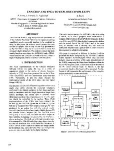
B. Backbone Network Size The minimum-size backbone network in a 1500 m x 1500 m operational area is illustrated in Fig. 7. (Note that the radio transmission range is about 300m based on the scenario setup in the simulator.) A minimum disk covering approach has been applied to approximate the minimum size of the BNet. This lower bound is obtained under the assumption that the nodes are uniformly distributed in the area, so that the backbone network needs to cover the entire operational area. Assuming we can choose the optimum location for the backbone nodes (BNs) to cover the whole area and form a connected BNet, the minimum size of this optimally positioned BNet is 19 BNs. Note that this lower bound is not achievable by simulation because in the simulation scenarios, the BNs are selected among existing nodes that are randomly distributed in the area.

Dai and Wu’s algorithm utilizes 2-hop neighborhood information while MBN ETSA only uses 1-hop neighborhood and 2-hop BN neighborhood information. There is always a tradeoff between the extent of neighborhood knowledge and the backbone size: The more neighborhood knowledge acquired, the smaller the resulting backbone. Surprisingly, the sizes of the backbone networks constructed by MBN ETSA and by Dai and Wu’s algorithm are almost the same in static network cases. In the mobile network cases, ETSA yields a slightly larger backbone because ETSA is designed to make sure the backbone network is connected first before any BN-toBCN conversion takes place. C. Control Message Overhead In Fig. 9, the average number of BN neighbors per node obtained by ETSA with Rule 1 and Rule 2 is about 6 BNs in static network cases, nicely under the theoretical bound of 22. Even in the mobile network cases, the average number of BN neighbors per node is less than 8 BN. We can conclude that the average number of BN neighbors per node is independent of the network size or of the nodal degree in the network.

The average size of the backbone network during simulation execution is shown in Fig. 8. In the static network cases shown in Fig. 8 (a), with BCN-to-BN restricting Rule 1 and Rule 2, the size of the backbone network (about 30 BNs) stays the same while the nodal density increases. On the other hand, the topology synthesis algorithm without any restricting rules produces a backbone network that is 7 times larger (200 BNs) when there are 500 nodes in the network, due to high nodal density induced control message losses. In the mobile network cases shown in Fig. 8 (b), the BNet size is smaller than for the static network cases because the nodes tend to move toward the center of the operational area. Less BNs are needed to cover all the nodes.

Since the Hello message length of ETSA depends only on the number of BN neighbors, we can conclude that the length of the ETSA-generated Hello messages is of the order of O(1). The simulation results shown in Fig. 10 illustrate this feature. On the other hand, Dai and Wu’s algorithm generates a much larger control message overhead (per node) due to the full 1hop neighbor list exchange requirement. The average nodal degree, i.e., the number of 1-hop neighbors, increases along with the network density, but the average nodal degree of the backbone network stays about the same. Therefore, we can

In both static and mobile network cases, applying only Rule 1 or only Rule 2, the backbone network size increases along with nodal density. However, the size of the backbone network stays the same while the nodal density increases, i.e., the

291

conclude that ETSA introduces a much smaller control message overhead than Dai and Wu’s algorithm does by requiring only 1-hop BN neighbor list exchange. Furthermore, with only 1-hop neighborhood and 2-hop BN neighborhood information, the size of the backbone network constructed by ETSA is almost the same as the one constructed by Dai and Wu’s algorithm. Backbone Network Size

Backbone Network Size 200

140

160

120 100 80 60

140 120 100 80 60

40

40

20

20

0 100

200

Unrestricted w/ Rule 1 w/ Rule 2 w/ Rule 1 & 2 Minimum Dai & Wu

180

Number of BNs

160

Number of BNs

200

Unrestricted w/ Rule 1 w/ Rule 2 w/ Rule 1 & 2 Minimum Dai & Wu

180

D. Algorithm Convergence Time In Fig. 11, the convergence time (in terms of the number of cycles) of the enhanced MBN topology synthesis algorithm for static networks is shown. Note that the convergence time we obtained here is independent of the values we chose for Short_Timer and Long_Timer, since we present the convergence time results in terms of the number of “cycles” (1 cycle = 1 Long_Timer period). We can see that on average, the topology synthesis algorithm proposed in this paper (with two restricting rules) converges in less than 8 cycles, nicely under the theoretical bound, 12. When only Rule 2 is applied, the convergence time is longer, bounded by 25. When only Rule 1 is applied, the algorithm convergences in 5 cycles, but generates a bigger BNet than when both rules are applied.

300

Number of Nodes

400

0 100

500

(a) Static network

200

300

Number of Nodes

400

On the other hand, Dai and Wu’s algorithm also converges in O(1) time, i.e. it takes less than 5 cycles.

500

(b) Mobile network

E. Throughput Performance For throughput performance evaluation, we impose 25 simultaneous UDP traffic flows with randomly selected disjoint source and destination nodes. The inter-arrival time of packets follows an exponential distribution with an average interarrival time of 0.21 sec; the packet size is set to 512 Bytes, leading to an offered traffic rate of 487.6 kbps. Based on the MBN structure described above, we modify the AODV routing algorithm, yielding a Mobile Backbone Network Routing (MBNR) protocol, by imposing the following requirement: only BNs (elected by ETSA) forward route request (RREQ) packets. In this way, a source node that becomes active will search for a route by distributing route request packets only across the BNet. For a fair comparison, a similar approach is used for Dai and Wu’s algorithm: only backbone nodes (elected by Dai and Wu’s algorithm) forward route request (RREQ) packets

Figure 8. Backbone network (BNet) size Average Number of BN Neighbors

Average Number of BN Neighbors 40 Unrestricted w/ Rule 1 w/ Rule 2 w/ Rule 1 & 2 Upper bound

35 30 25 20 15 10 5 0 100

200

300

400

Unrestricted w/ Rule 1 w/ Rule 2 w/ Rule 1 & 2 Upper bound

35

Number of BN Neighbors

Number of BN Neighbors

40

30 25 20 15 10 5 0 100

500

200

300

400

500

Number of Nodes

Number of Nodes

(a) Static network

(b) Mobile network

Figure 9. Number of BN neighbors Hello Message Rate (per node) 2.0 1.6 1.4

Unrestricted w/ Rule 1 w/ Rule 2 w/ Rule 1 & 2 Dai & Wu

1.8 1.6

Rate (Kbps)

1.8

1.2 1.0 0.8 0.6 0.4

1.4

We observe that the use of AODV as the primary routing protocol in a wireless mesh network does not provide a scalable approach when the network size is large and/or the nodal density is high. The simulation results shown in Fig. 12 indicate that as the nodal density increases, the data delivery ratio of AODV deteriorates and so does MBNR without restricted by Rule 1 and Rule 2. The high rate of generated RREQ packets (illustrated in Fig. 13) imposes a network overload, which leads to the observed throughput degradation. The excessive MAC contention induced by this heavy loading further exacerbates the situation.

1.2 1.0 0.8 0.6 0.4

0.2

0.2

0.0 100

200

300

Number of Nodes

400

500

0.0 100

(a) Static network

200

300

Number of Nodes

400

500

(b) Mobile network

Figure 10. Control message (Hello message) overhead per node Convergence Time 25

Unrestricted w/ Rule 1 w/ Rule 2 w/ Rule 1 & 2 w/ Rule 1 & 2 bound Dai & Wu

20

Number of Cycles

Rate (Kbps)

Hello Message Rate (per node) 2.0

Unrestricted w/ Rule 1 w/ Rule 2 w/ Rule 1 & 2 Dai & Wu

On the other hand, both ETSA with two restricting rules and Dai and Wu’s algorithm yield over 95% data delivery ratio in static network cases. In mobile network cases, ETSA yields over 95% delivery ratio, while the delivery ratio of Dai and Wu’s algorithm decreases when the nodal density is high, i.e., drops to 75% when the network contains 500 nodes. ETSA achieves higher data delivery ratio than Dai and Wu’s algorithm does because ETSA has much lower control overhead (Hello message sending rate) and ETSA is designed to yield a backbone network with richer connectivity in mobile environment.

15 10 5 0 100

200

300

400

500

Number of Nodes

Figure 11. Convergence time

The average path length of the 25 UDP traffic flows is shown in Fig. 14. Surprisingly, AODV does not produce 292

shorter path lengths even with a 100% data delivery rate (as MBNR does). When a network experiences a high rate of data loss, many RREQ packets are also dropped, leading to long (“non-shortest”) paths being selected by AODV. While theoretically MBNR can induce a path length which is up to 5 hops longer, this rarely occurs. MBNR with only rule 2 applied produces a slightly shorter (< 5%) path length. This small difference can be seen in the static network cases.

Average End-to-End Delay

Delay (s)

2.0

80

80

60

AODV w/ Rule 1 & 2 Dai & Wu Unrestricted w/ Rule 1 w/ Rule 2

40 20 0 100

200

300

400

Number of Nodes

60

20 0 100

500

(a)Static network

200

300

400

Number of Nodes

1000000

Number of RREQ

1000000

Number of RREQ

10000000

AODV w/ Rule 1 & 2 Dai & Wu Unrestricted w/ Rule 1 w/ Rule 2

10000

400

500

100

500

200

300

400

Number of Nodes

500

5.0

7.0

AODV w/ Rule 1 & 2 Dai & Wu Unrestricted w/ Rule 1 w/ Rule 2

6.5 6.0

4.5 4.0 3.5 3.0

[1]

5.5 5.0

AODV w/ Rule 1 & 2 Dai & Wu Unrestricted w/ Rule 1 w/ Rule 2

[2]

4.5 4.0 3.5 3.0

2.5 2.0 100

2.5

200

300

Number of Nodes

400

(a)Static network

300

400

500

Number of Nodes

(b) Mobile network

CONCLUSIONS

REFERENCES

Average Path Length

Number of Hops

Number of Hops

5.5

200

(b) Mobile network

Average Path Length

6.0

0.0 100

This work was supported by Office of Naval Research (ONR) under Contract No. N00014-01-C-0016, as part of the AINS (Autonomous Intelligent Networked Systems) project, by the National Science Foundation (NSF) under Grant No. ANI-0087148. and by University of California/Conexant MICRO Grant No. 04-100.

10000

(a)Static network

6.5

500

ACKNOWLEDGMENT

Figure 13. Total number of RREQ packets forwarded in the network

7.0

400

In this paper, an enhanced Mobile Backbone Network (MBN) topology synthesis algorithm (ETSA) is presented. Two BCN-to-BN conversion restricting rules are introduced to regulate excessive BCN-to-BN conversions induced by imperfect neighborhood information from control message losses and asynchronous operation. The combination of Rule 1 and Rule 2 yields stable and robust operation of ETSA. The backbone network consists of a sufficient but not excessive number of nodes, and the BNet size is independent of the nodal density of the network. This MBN structure significantly reduces routing overhead while negligibly increasing the average path length. Furthermore, the same desirable analytical features are retained—constant (O(1)) convergence time and constant (O(1)) control message length. In comparison with other time-efficient connected dominating set (CDS) formation algorithms, ETSA elects a sufficient but not excessive number of backbone nodes with very limited neighborhood information and with very little communication overhead, i.e., only 1-hop BN neighbor list exchange is required.

1000

300

300

VI.

AODV w/ Rule 1 & 2 Dai & Wu Unrestricted w/ Rule 1 w/ Rule 2

100000

1000

Number of Nodes

200

Number of RREQ Forwarded

Number of RREQ Forwarded

200

1.0

Figure 15. Average end-to-end delay

(b) Mobile network

10000000

100

1.5

0.5

(a)Static network

Figure 12. Data packet delivery ratio

100000

1.0

Number of Nodes

AODV w/ Rule 1 & 2 Dai & Wu Unrestricted w/ Rule 1 w/ Rule 2

40

2.0

1.5

0.0 100

AODV w/ Rule 1 & 2 Dai & Wu Unrestricted w/ Rule 1 w/ Rule 2

2.5

0.5

Data Delivery Ratio 100

Delievery Ratio (%)

Delievery Ratio (%)

Data Delivery Ratio

3.0

AODV w/ Rule 1 & 2 Dai & Wu Unrestricted w/ Rule 1 w/ Rule 2

Delay (s)

2.5

Finally, we also observe that mobility can help shorten average path length because source and destination nodes may move closer to each other. Note that Dai and Wu’s algorithm produces a slightly longer average path length because (1) not enough backbone nodes are elected and (2) the algorithm lacks a mechanism to limit the path length. Longer average path length also results in longer average end-to-end delay as illustrated in Fig. 15. High control overhead induced by Dai and Wu’s algorithm also contributes to the worse delay performance. One readily observes that, in static network scenarios, the average end-to-end delay of Dai and Wu’s algorithm can go up to 1.2s while the average end-to-end delay of ETSA stays under 0.3s.

100

Average End-to-End Delay

3.0

500

2.0 100

[3] 200

300

Number of Nodes

400

500

(b) Mobile network

[4]

Figure 14. Average Path Length

293

I. Rubin, A. Behzad, H. Ju, R. Zhang, X. Huang, Y.-C. Liu, R. Khalaf, “Ad Hoc Wireless Networks with Mobile Backbones”, Proceedings of IEEE International Symposium on Personal, Indoor and Radio Communications (PIMRC), vol.1, pages: 566 – 573, 2004. H. Ju, I. Rubin, K. Ni, C. Wu, “A Distributed Mobile Backbone Formation Algorithm for Wireless Ad Hoc Networks”, Proceedings of IEEE International Conference on Broadband Networks (BroadNets), pages: 661-670, 2004. K. Alzoubi, X.-Y. Li, Y. Wang, P.-J. Wan and O. Frieder, ”Geometric Spanners for Wireless Ad Hoc Networks”, IEEE Transactions on Parallel and Distributed Systems”, vol. 14 , pages: 408 - 421, April 2003 R. Sivakumar, P. Sinha, and V. Bharghvan, “CEDAR: A CoreExtraction Distributed Ad Hoc Routing Algorithm”, IEEE Journal on

Selected Area in Communications, Vol. 17, No. 8, pages: 1454 – 1465, August 1999 [5] L. Bao and J.J. Garcia-Luna-Aceves, “Topology Management in Ad Hoc Networks”, Proceedings of the 4th ACM international symposium on Mobile ad hoc networking and computing (MobiHoc), pages: 129 – 140, 2003 [6] F. Dai and J. Wu, “An Extended Localized Algorithm for Connected Dominating Set Formation in Ad Hoc Wireless Networks”, IEEE Transactions on Parallel and Distributed Systems, vol. 15, pages: 908 – 920, Oct. 2004 [7] K. Alzoubi, P. Wan, and O. Frieder, “Message-Optimal Connected Dominating Sets in Mobile Ad Hoc Networks”, Proceedings of the 3rd ACM international symposium on Mobile ad hoc networking and computing (MobiHoc), pages: 157 – 164, 2002 [8] S. Dhar, M. Q. Rieck, S. Pai, and E. J. Kim, “Distributed Routing Schemes for Ad Hoc Networks Using d-SPR Sets”, Journal of Microprocessors and Microsystems, Special Issue on Resource Management in Wireless and Ad Hoc Mobile Networks, Oct. 2004. [9] J. Wu and H. Li, “On Calculating Connected Dominating Set for Efficient Routing in Ad Hoc Wireless Networks”, Proc. of the Third International Workshop on Discrete Algorithms and Methods for Mobile Computing and Communications, 1999 [10] U. C. Kozat, G. Kondylis, B. Ryu and M. K. Marina, “Virtual Dynamic Backbone for Mobile Ad Hoc Networks”, Proceedings of IEEE

[11]

[12]

[13] [14]

[15]

[16] [17]

294

International Conference on Communications (ICC), Vol. 1, pages 250 – 255, June 2001 W. Lou and J. Wu, “A Cluster-Based Backbone Infrastructure for Broadcasting in MANETs”, Proc. of Workshop on Wireless, Mobile, and Ad Hoc Networks (in conjunction with IPDPS), April 2003 M. Mosko, J.J. Garcia-Luna-Aceves, C. Perkins, “Distribution of Route Requests Using Dominating-Set Neighbor Elimination in an On-demand Routing Protocol”, Proceedings of IEEE GlobeCom, vol. 2, pages: 1018 – 1022, Dec. 2003 Wireless LAN Medium Access Control (MAC) and Physical Layer (PHY) Specifications, IEEE 802.11, 1999 I.F. Akyildiz, X. Wang, and W. Wang, ``Wireless Mesh Networks: A Survey,'' Computer Networks Journal (Elsevier), Vol. 47, pages 445487, March 2005. P. Bahl, A. Adya, J. Padhye, A. Wolman, “Reconsidering Wireless Systems with Multiple Radios”, ACM SIGCOMM Computer Communication Review, vol. 34, pages 39 – 46, Oct. 2004 J. Hauser, D. Baker, W. S. Conner, Draft PAR for IEEE 802.11 ESS Mesh, IEEE Document Number: IEEE 802.11-04/054r2 A. Qayyum, L. Viennot, and A. Laouiti, “Multipoint Relaying for Flooding Broadcast Messages in Mobile Wireless Networks”, Proceeding of HICSS, pages 3866 – 3875, 2002