Maximum Likelihood Eigenspace and MLLR for Speech Recognition in Noisy Environments Patrick Nguyen http://www.eurecom.fr/˜nguyenp

Christian Wellekens

Jean-Claude Junqua

[email protected]

[email protected]

Institut Eur´ecom, Sophia-Antipolis, France Speech Technology Laboratory, Santa Barbara, California, USA Abstract– A technique for rapid speaker adaptation, called eigenvoices, was introduced recently. The key idea is to confine models in a very low-dimensional linear vector space. This space summarizes a priori knowledge that we have about speaker models. In many practical systems, however, there is a mismatch between the conditions in which the training data were collected and test conditions: prior knowledge becomes improper. Furthermore, prior statistics or models of this mismatch may not be available. We expose two key results: first, we use a maximum-likelihood estimator of prior information in matched conditions, called MLES, leading to an improvement of adaptation by a relative %, and second, we show how we can apply a blind scheme for learning noise, MLLR, achieving an additional % relative improvement in noisy conditions. I. I NTRODUCTION This paper aims at addressing one very frequent objection to eigenvoices [1]: we either do not have enough speakers, or not enough data for each speaker to build reasonable speaker-dependent (SD) models, or both. While we successfully applied eigenvoices in a framework where data was reduced [2], these preliminary results might not apply to all cases. Our work here brings a viable solution by describing a methodology for initializing eigenvoices in an environment where one has enough data and transposing it to a new problem where data are scarce. The following is organized as is: in the remainder of the section, we define the problem and give an overview of the solution. The next section is dedicated to defining eigenvoices and MLLR. Then we devote the next section to the normalization of the eigenspace to a new environment. Experiments complement our theory. A. Problem definition We find ourselves in the following context: we want to perform very fast speaker adaptation in a noisy speech environment. It has now become common belief that use of prior information helps in deriving constraints that reduce the number of parameters to be estimated. However, this is incompatible with our other aim, namely, working in an environment where it is hard to collect data. Building good prior information requires a significant amount of data that is not available for the noisy speech recognition task. Consider the following example: we want to develop a car navigation system. The system is trained with publicly available databases such as TIMIT, which contains sufficient data to

train prior parameters. However, the latter becomes almost completely useless as we move to our target task. We need fast speaker adaptation for user convenience, but it cannot be deployed in the new environment. B. General idea To solve this problem, we record a small database in real conditions. We model the transformation to the new environment as an affine transformation. We must be careful not to include information that is specific to the speakers in the small database into the transformation. Once we have our mapping from training to test conditions, we apply it to our prior knowledge, which can now be readily used for fast speaker adaptation with new speakers in real conditions. II. A DAPTATION METHODS We present two adaptation methods in this section: eigenvoices and MLLR. We only introduce matter that is useful for further purposes in our paper and the reader is assumed to have had prior exposure to the methods. A. Eigenvoices In this section, we briefly describe eigenvoices. We merely provide the reader with basic definitions, and further information can be found in [1]. The basic idea is that we can infer strong a priori knowledge about a speaker’s location in the space of its HMM parameters. We observe training speakers and given their distribution in the dimensional space of their HMM parameters, we find the dimensional linear vector space that minimizes the Euclidean out-of-space distance using principal component analysis (PCA [3]). We call the latter the eigenspace. We only perform adaptation of the mean vectors. A.1 Optimal location of speaker (MLED) We now describe how to find the maximum-likelihood eigendecomposition (MLED), that is the location in the eigenspace that maximize the likelihood of an utterance given the model. Let be the parameter vector of a speaker, and be the basis vectors of the eigenspace, called eigenvoices. Then we have

where are the eigenvalues that represent the characteristics of the speaker, and is the eigenspace. We use the EM-algorithm [4] to find the

maximum-likelihood for the observation :

eigendecomposition

(MLED)

Finding requires the inversion of an matrix. Specifying that the speaker is confined in the eigenspace is a hard constraint. We can relax the constraint by assuming a normal-Wishart density around the MLED estimate. We can thus use MAP ([5], [6]) as a postprocessor with MLED as prior. A.2 Maximum-Likelihood EigenSpace We now derive a straightforward method to find a compact eigenspace. The method is called maximum-likelihood eigenspace (MLES). It serves several purposes. First, PCA requires heavy memory requirements that might be too demanding for large vocabulary continuous speech recognition systems. Second, it is not based on a distributionto-distribution divergence measure that requires gaussians within a mixture gaussian to be aligned. Third, it leverages the need to build speaker-dependent (SD) models for each speaker: building SD models and then applying PCA corresponds to going from a -dimensional parameter estimation (SI) to a problem (building SD models), and then reducing dimension from to . We solve the problem directly. MLES works on only times more degrees of freedom than training of the speakerindependent (SI) model. Lastly, MLES enables us to integrate a certain form of prior knowledge by explicitly setting eigenvalues. We just integrate eigenvalues as hidden data in the estimation problem, yielding (1) where contains prior information about speaker (e.g. the probability of a person of a given dialect or sex to appear). It is extensively used for unbalanced sets of speakers. For instance, we may set for a given if and qth speaker is male if and qth speaker is female elsewhere

Seed eigenvoices can be obtained through PCA or linear discriminant analysis (LDA). When no particular knowledge about is known, we use MLED to replace the integration operator by a maximum operator. The reestimation formula is relatively easy to derive

(2)

where eigenvoice.

represent a speaker, a distribution, and an is the posterior probability of the utterances

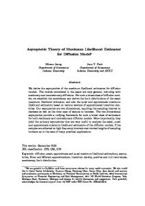
of the speaker, . is the observed posterior probability. is the current estimate of the th eigenvalue of speaker . Finally, is the complement of the estimated mean, ie (3) The training algorithm is very akin to a Baum-Welch procedure, except for the fact that we keep accumulators instead of just one. Its seems that our algorithm converges approximately two times slower than training of the simple SI model. Note that PCA gives the least-squares estimate for the eigenspace and therefore is suboptimal in the light of the ML-criterion. For consistency, we will now refer to the space found by PCA as least-squares eigenspace (LSES). Figure 1 compares the histograms for three ways of obtaining the eigenspace: LSES, MLES, and MAPES (MLES using prior information about the number of males and females in the database). See section IV.B for more details. A.3 Properties We now discuss the properties of interest of eigenvoices. We have an explicit model of the variabilities of speakers. These are formed individually by vectors call eigenvoices, each of which models a direction of variation. These eigenvoices constitute prior knowledge we have about speakers and have been optimized given a set of speakers in some given homogeneous conditions. Hence, we are now able to make very strong assumptions about where a speaker model can reside, and consequently achieve very fast adaptation, but on the other hand our prior knowledge is very specialized to the training set. B. Maximum-Likelihood Linear Regression B.1 Definition Maximum-likelihood linear regression (MLLR) finds the optimal affine transformation of a model [7]. Gaussian mean parameters are pooled into regression classes. Let be one of the mean vectors in regression class . Then

and and are the transformation parameters of class . MLLR can also be applied in the observation features space by simply inverting the transformation: this can be seen as a normalization of the features. In this paper, we only consider one global transformation. The very interesting property of this technique is that no prior knowledge is required except that of the assignment of regression classes. Therefore, MLLR seems very suitable as a constrained, indirect method to adapt to noise. We apply MLLR in the feature space. Let and be the accumulators. Then the normalized accumulators become

20 15

= 29.582

10 5 0

0

20

40

60

80

(a) Least-squares eigenspace (LSES): this is the seed eigenspace. The eigenvalue does not represent sex perfectly. 2.82% of speakers for which the sign of the eigenvalue is positive for a female or negative for a male. 20 15

= 24.6279

10 5 0

0

20

40

60

80

(b) Maxmimum-likelihood eigenspace (MLES): after 3 iterations of Baum-Welch training, differences between sexes are blurred. 5.41% of speakers now bear a misleading sign of eigenvalue 20 15

= 32.3265

10 5 0

0

20

40

60

80

(c) Maximum-a-posteriori eigenspace (MAPES): after 3 iterations, there is now only 1.95% of speakers with wrong sign of eigenvalue. Means of the male and female distributions are converging to the same absolute value.

Fig. 1. Sex and first eigenvalue: histograms. Male and female speakers are shown in grey and black respectively.

B.2 Properties MLLR is a transformation-based adaptation method. No prior knowledge except SI models and the regression class topology are required. It uses a small set of indirect parameters and therefrom reliable adaptation can be improved. Also, it works equivalently with environment and speaker adaptation. III. N ORMALIZING THE EIGENSPACE

WITH RESPECT TO AN UNKNOWN ENVIRONMENT

This section explains into more details about how we normalize the eigenspace for use with a new environment. We assume the following: (1) we trained an eigenspace on a large database , (2) we have collected a small amount of data in real-life conditions in , and (3) we have test data recorded in , in the same conditions as . The algorithm can be decomposed in three steps: 1. For each speaker in , perform MLED. MLED projects the speaker in the reference space. MLLR will compute a transofrmation between the data from the reference space and the noisy space for all speakers, making the transformation to focus on environmental variations only. Compute the contribution of the speaker’s utterances in the MLLR system.

2. Compute transformation modelling the environment. Now we work with an environment-dependent SI. 3. For each speaker in , perform MLED in the reference space, then rescale estimate (apply MLLR). IV. E XPERIMENTS A. Configuration The experiments were conducted on the TIMIT database, using the standard train/test partition. There are 462 speakers in the training set (325 males) and 169 in the test set. Each speaker pronounces 8 sentences of a length of about 2-7 sec each. Speech was sampled at 16 kHz and parameterized using PLP cepstral features without cepstral filtering. There are 9 static coefficients (including energy of the residual) and 9 delta, totalling 18 features. We use 48 context-independent HMM models, with 3 emitting states and 16 gaussians per mixture, resulting in 2240 distributions. Adaptation is supervised. Noise of a car running at 60 mph was added artificially to the utterances. No noise reduction processing was applied and a bigram grammar was used. In the following, we report results in unit accuracy. The SNR for clean TIMIT is about 70 dB.

Size / SNR:

Method LSES MLES( MLES( MLES(

60.67 62.53 63.06 61.74

) ) )

60.58 65.10 65.01 63.77

61.29 65.37 64.84

)

60.94 59.79 53.14 65.05 64.25

40 dB 50.13 56.86 52.44 57.13 62.53

30 dB 31.09 44.82 42.78 43.14 52.08

40 dB 62.53 61.65 60.83 60.35

30 dB 52.08 51.37 53.28 50.74

20 dB 34.54 33.78 33.08 32.91

TABLE III: R EDUCING DATA FOR ENVIRONMENT NORMALIZATION

TABLE I: M AXIMUM - LIKELIHOOD EIGENSPACE

Method/SNR SI ( ) MLLR( ) LR ( ) EV ( ) normEV ( ,

64.25 64.46 63.59 63.52

61.56 66.96

20 dB 10.63 30.82 25.07 19.31 34.54

TABLE II: R ESULTS FOR DIFFERENT SNR S

B. MLES vs LSES Table I evidences the performance of the maximumlikelihood criterion vs least-squares. MLES was applied for different values of (first column) and tested the eigenspaces with other values of (first row). LSES served as the seed eigenspace for MLES. Due to memory limitations, LSES was estimated on a set of only 100 speakers, but balanced with respect to sex. MLES used all 462 speakers. Obviously, MLES performs best when with more dimensions and when we test with the same number of dimensions with which we trained the eigenspace. This means that we have to know in advance how many dimensions we want to use in our system when building prior information. C. Normalization We expose results in table II. comprised 30 speakers, each pronouncing 8 sentences. was made up by 30 speakers, each pronouncing 1 sentence (about 2-7 sec of speech) for adaptation and the rest for decoding . All results reported are on . SI ( ) represents the SI model, estimated on the full training set of the TIMIT database. MLLR( ) can be interpreted as the SI normalized by the environment learned from . MLLR( ) and MLED( ) correspond to MLLR and MLED applied normally, without any use of . Finally, normEV( , ) symbolizes MLED applied on with priors transformed using an estimation of the environment based on . These sets were sliced randomly (non-overlapping) from the test set of TIMIT. For all tests, was set to 10. D. Further experiments: reducing amount of data In a further experiment, we examine how the algorithm reacts when we reduce the size of the re-training database, . Table III summarizes the results. The first column describes the size of the database by the product of the number of speakers times the number of utterances per speaker. We see that it is better to have less speakers, but each pronouncing more utterances, than more speaker with less utterances.

V. C ONCLUSION In this paper, we have showed how eigenvoices can be used in practical real-life environments. The contribution of this work is twofold: first, we demonstrate that the eigenspace can be trained in an optimal way without requiring enough data per speaker to build SD models, and second, we lay out a method to transpose the eigenspace from a clean to a noisy environment. We have illustrated why the use of prior densities is useful to guide the training of the eigenspace, and observed significant performance improvements of MLES versus LSES. Also, MLES has very low memory requirements (only times those required for SI training). Additionally, MLES does not require sufficient data per speaker to build SD models: we only need about times more data than needed to build SI models. Convergence of the EM-algorithm is not times slower but takes approximately twice as much iterations as embedded reestimation of SI models. We have also unveiled a practical method that allows reuse of the eigenspace in unmatched conditions using a very small pool of re-training data. We have specifically separated environment variabilities from speaker variabilities. The eigenspace that was trained on clean speech was normalized and subsequently produced accurate constraints for speakers in the noisy environment. Thereby, we could again achieve fast speaker adaptation (about 2-7 sec per speaker) in an unmatched environment. R EFERENCES R. Kuhn, P. Nguyen, J.-C. Junqua, L. Goldwasser, N. Niedzielski, S. Fincke, K. Field, and M. Contolini, “Eigenvoices for speaker adaptation,” ICSLP, vol. 5, pp. 1771–1774, 1998. [2] R. Kuhn, P. Nguyen, J.-C. Junqua, R. Boman, N. Niedzielski, S. Fincke, K. Field, and M. Contolini, “Fast Speaker Adaptation in Eigenvoice Space,” ICASSP, vol. 2, pp. 749–752, 1999. [3] I. T. Jolliffe, Principal Component Analysis, Springer-Verlag, 1986. [4] A.P. Dempster, N.M. Laird, and D.B. Rubin, “Maximum-Likelihood from Incomplete Data via the EM algorithm,” Journal of the Royal Statistical Society B, pp. 1–38, 1977. [5] J.-L. Gauvain and C.-H. Lee, “Maximum a posteriori estimation for multivariate Gaussian mixture observations of Markov Chains,” IEEE Tr. on Speech and Audio Proc., vol. 2, no. 2, pp. 291–298, Apr. 1994. [6] J.-L. Gauvain and C.-H. Lee, “Bayesian Learning for Hidden Markov Model with Gaussian Mixture Observation of Markov Chains,” Speech Communication, vol. 11, pp. 205–213, 1992. [7] C. J. Leggetter and P. C. Woodland, “Maximum likelihood linear regression for speaker adaption of continuous density hidden Markov models,” Computer Speech and Language, vol. 9, pp. 171–185, 1995. [8] R. Kuhn, P. Nguyen, J.-C. Junqua, L. Goldwasser, N. Niedzielski, S. Fincke, and K. Field, “Eigenfaces and eigenvoices: dimensionality reduction for specialized pattern recognition,” MMSP, pp. 71–76, 1998. [9] C. J. Leggetter and P. C. Woodland, “Speaker Adaptation of HMMs using Linear Regression – TR.181,” Tech. Rep., Cambridge University Engineering Department, June 1994. [10] M. J. F. Gales, “Maximum Likelihood Linear Transformations for HMM-based Speech Recognition – TR.291,” Tech. Rep., Cambridge University Engineering Department, May 1997. [1]