PHYSICAL REVIEW E 71, 046141 共2005兲
Maximal planar networks with large clustering coefficient and power-law degree distribution Tao Zhou,1,2 Gang Yan,2 and Bing-Hong Wang1,*
1
Nonlinear Science Center and Department of Modern Physics, University of Science and Technology of China, Hefei Anhui, 230026, People’s Republic of China 2 Department of Electronic Science and Technology, University of Science and Technology of China, Hefei Anhui, 230026, People’s Republic of China 共Received 30 September 2004; revised manuscript received 21 December 2004; published 28 April 2005兲 In this article, we propose a simple rule that generates scale-free networks with very large clustering coefficient and very small average distance. These networks are called random Apollonian networks 共RANs兲 as they can be considered as a variation of Apollonian networks. We obtain the analytic results of power-law 46 3 exponent ␥ = 3 and clustering coefficient C = 3 − 36 ln 2 ⬇ 0.74, which agree with the simulation results very well. We prove that the increasing tendency of average distance of RANs is a little slower than the logarithm of the number of nodes in RANs. Since most real-life networks are both scale-free and small-world networks, RANs may perform well in mimicking the reality. The RANs possess hierarchical structure as C共k兲 ⬃ k−1 that are in accord with the observations of many real-life networks. In addition, we prove that RANs are maximal planar networks, which are of particular practicability for layout of printed circuits and so on. The percolation and epidemic spreading process are also studied and the comparisons between RANs and Barabási-Albert 共BA兲 as well as Newman-Watts 共NW兲 networks are shown. We find that, when the network order N 共the total number of nodes兲 is relatively small 共as N ⬃ 104兲, the performance of RANs under intentional attack is not sensitive to N, while that of BA networks is much affected by N. And the diseases spread slower in RANs than BA networks in the early stage of the suseptible-infected process, indicating that the large clustering coefficient may slow the spreading velocity, especially in the outbreaks. DOI: 10.1103/PhysRevE.71.046141
PACS number共s兲: 89.75.Hc, 64.60.Ak, 84.35.⫹i, 05.40.⫺a
I. INTRODUCTION
Many social, biological, and communication systems can be properly described as complex networks with nodes representing individuals or organizations and edges mimicking the interactions among them 关1–14兴. Examples are numerous: these include the Internet 关15–17兴, the World Wide Web 关18–22兴, social networks of acquaintance or other relations between individuals 关23–34兴, metabolic networks 关35–39兴, food webs 关40–46兴, and many others 关47–58兴. The ubiquity of complex networks inspires scientists to construct a general model. In the past 200 years, the study of topological structures of the networks used to model the interconnection systems has gone through three stages. For over a century, there was an implicit assumption that the interaction patterns among the individuals can be embedded onto a regular structure such as Euclidean lattices, hypercube networks, and so on 关59–62兴. Since late 1950s mathematicians began to use random graphs to describe the interconnections, this is the second stage 关63–70兴. In the past few years, with the computerization of data acquisition process and the availability of high computing powers, scientists have found that most real-life networks are neither completely regular nor completely random. The results of many empirical studies and statistical analyses indicate that the networks in various fields have some common characteristics, the most important of which are called small-world effect 关71–76兴 and scale-free property 关77–80兴.
*Electronic address:
[email protected] 1539-3755/2005/71共4兲/046141共12兲/$23.00
In a network, the distance between two nodes is defined as the number of edges along the shortest path connecting them. The average distance L of the network, then, is defined as the mean distance between two nodes, averaged over all pairs of nodes. The average distance is one of the most important parameters to measure the efficiency of communication networks. For instance, in a store-forward computer network, probably the most useful measurement of its performance is the transmission delay 共or time delay兲 encountered by a message traveling through the network from its source to destination; this is approximately proportional to the number of edges a message must pass through. Thus the average distance plays a significant role in measuring the transmission delay. The number of edges incident from a node x is called the degree of x, denoted by k共x兲. Obviously, through the k共x兲 edges, there are k共x兲 nodes that are correlated with x; these are called the neighbor set of x, and denoted by A共x兲. The clustering coefficient C共x兲 of node x is the ratio between the number of edges among A共x兲 and the total possible number; the clustering coefficient C of the whole network is the average of C共x兲 over all x. Empirical studies indicate that most real-life networks have much smaller average distance 共as L ⬃ ln N where N is the number of nodes in the network兲 than the completely regular networks and much greater clustering coefficient than those of the completely random networks. Therefore they should not be treated as either completely regular or random networks. The recognition of small-world effect involves the two factors mentioned above: a network is called a small-world network as long as it has small average distance and great clustering coefficient. Another important characteristic in real-
046141-1
©2005 The American Physical Society
PHYSICAL REVIEW E 71, 046141 共2005兲
ZHOU, YAN, AND WANG
life networks is the power-law degree distribution, that is p共k兲 ⬀ k−␥, where k is the degree and p共k兲 is the probability density function for the degree distribution. ␥ is called the power-law exponent, and is usually between 2 and 3 in reallife networks 关1–3兴. This power-law distribution falls off much more gradually than an exponential one, allowing for a few nodes of very large degree to exist. Networks with power-law degree distribution are referred to as scale-free networks, although one can and usually does have scales present in other network properties. From 1998 much attention has been focused on how to model a complex network. One of the most well-known models is Watts and Strogatz’s small-world network 共WS network兲, which can be constructed by starting with a regular network and randomly moving one endpoint of each edge with probability p 关72兴. Another popular model was proposed independently by Monasson 关75兴 and by Newman and Watts共NW networks兲 关74兴, where no edges are rewired. Some variations of the small-world model have been proposed. Several authors have studied the model in dimension higher than one and obtained similar results to the one dimension case 关74,81–84兴. Another kind of model in which shortcuts preferentially join nodes that are close together on the underlying lattice also have been studied 关85–87兴. Very recently, Zhu et al. proposed a so-called directed dynamical small-world model, in which the network structure is affected by the processes upon the network 关76兴. Another significant model is Barabási and Albert’s scalefree network model 共BA network兲 关77,78兴, which is very similar to Price’s 关79,80兴. The BA model suggests that two main ingredients of self-organization of a network in a scalefree structure are growth and preferential attachment. These point to the facts that most networks grow continuously by adding new nodes, which are preferentially attached to existing nodes with a large number of neighbors. The subsequent researches on various processes taking place upon complex networks, such as percolation 关83,88–99兴, epidemic processes 关100–107兴, cascade processes 关108–116兴, and so on, indicate that the scale-free degree distribution may play the most crucial role rather than small-world effect. Therefore, in the past 2 or 3 years, the study of modeling complex networks focuses on revealing the underlying mechanism of power-law degree distribution. Roughly, these models for scale-free networks can be classified into three main scenarios. The first one is related to the models of human behavior 关117,118兴 and was introduced in a network version under the name “preferential attachment” mentioned above 关77,78,119–131兴. The second class of models is where a scale-free distribution appears as a result of a balance between a modeled tendency to form hubs against an entropic pressure towards a random network with an exponential degree distribution 关132–134兴. The third one is the selforganized models that lead to power-law degree distribution 关135–141兴. In the recent several months, a few authors have demonstrated the use of pure mathematical objects and methods to construct scale-free networks. One interesting instance is the so-called integer networks 关142兴, in which the nodes represent integers and two nodes x and y are linked by an edge if and only if x is divided exactly by y or y is divided exactly
by x, where x and y are nonzero integers. Zhou et al. have studied the statistical properties of these networks and demonstrated that they are scale-free networks of large clustering coefficient. Another significant instance is Apollonian network 共ANs兲 introduced by Andrade et al. 关143兴. In our opinion, Apollonian networks may be not the networks of best performance, but assuredly the most beautiful ones we have ever seen. Another related work is owed to Dorogovtsev and Mendes et al., in which the deterministic networks, named pseudofractals, are obtained by random attachment aiming at edges 关144,145兴. In this article, we propose a simple rule that generates scale-free networks with a very large clustering coefficient and very small average distance. These networks are called random Apollonian networks 共RANs兲, since they can be considered as a variation of Apollonian networks 关151兴. We discuss the difference between RANs and ANs in detail共in addition, the difference between RANs and BA networks兲, and demonstrate that RANs perform much better than BA networks in some aspects. This article is organized as follow: In Sec. II, the Apollonian networks are introduced. In Sec. III, the rule that generates RANs is described in detail. In Sec. IV, we give both the simulation and analytic results about the statistical characteristics of RANs, including the scale-free property and the small-world effect, where the detailed analytic processes are shown in the Appendixes. In Sec. V, we prove that RANs are the maximal planar networks. In Sec. VI, the percolation and epidemic spreading process are also studied and the comparisons between RANs and BA networks as well as NW networks are shown. Finally, we sum up this article and discuss the relevance of RANs to the real world in Sec. VII. II. BRIEF INTRODUCTION OF APOLLONIAN NETWORKS
Apollonian networks, introduced by Andrade et al. 关143兴, are derived from the problem of space-filling packing of spheres according to the ancient Greek mathematician Apollonius of Perga 关146兴. To produce an Apollonian packing, we start with an initial array of touching disks, the interstices of which are curvilinear triangles. In the first generation disks are added inside each interstice in the initial configuration, such that these disks touch each of the disks bounding the curvilinear triangles. The positions and radii of these disks can easily be calculated, and the circle size distribution follows a power law with an exponent of about 1.3 关146兴. Of course, these added disks cannot fill 1all of the space in the interstices, but instead give rise to three smaller interstices. In the second generation, further disks are added inside all of these new interstices, which again touch the surrounding disks. This process is then repeated for successive generations. If we denote the number of generations by t, where t = 0 corresponds to the initial configuration, as t → ⬁ the space-filling Apollonian packing is obtained as shown in Fig. 1. Apollonian packing can be used as a basis of a network, where each disk is a node in the network and nodes are connected if the corresponding disks are in contact. We call this contact an “Apollonian network.” Figure 2 shows how
046141-2
PHYSICAL REVIEW E 71, 046141 共2005兲
MAXIMAL PLANAR NETWORKS WITH LARGE…
FIG. 1. An Apollonian packing of disks within a circle 关147兴.
the network evolves with the addition of new nodes at each generation. For each new disk added, three new interstices in the packing are created, which will be filled in the next generation. Equivalently, for each new node added, three new triangles are created in the network, into which nodes will be inserted in the next generation. Doye et al. have studied the properties of Apollonian networks in detail 关147兴 and shown the degree distribution p共k兲 ⬀ k−␥, average length l ⬀ 共ln N兲, where ␥ = 1 + 共ln 3 / ln 2兲 ⬇ 2.585,  ⬇ 0.75 and N is the order 关148兴 of the network; in other words, Apollonian networks are scale free and display small-world effect. It is worth remarking that the clustering coefficient C is close to 0.828, much larger than that of BA networks, in the limit of large N. Andrade et al. have also found many peculiar results about some well-known models upon Apollonian networks, including percolation, electrical conduction, and a magnetic model 关143,150兴.
FIG. 3. 共Color online兲 The sketch maps for the network growing process. The four figures show a possible growing process for RANs at time t = 1 共a兲, t = 2 共b兲, t = 3 共c兲, and t = 4 共d兲. At time step 1, the fourth node is added to the network and linked to nodes 1, 2, and 3. Then, at time step 2, the triangle ⌬134 is selected, the fifth node is added inside this triangle and linked to nodes 1, 3, and 4. After that, the triangles ⌬234 and ⌬124 are selected at time steps 3 and 4, respectively. Nodes 6 and 7 are added inside these two triangles respectively. 共d兲 shows a random Apollonian network of order 7. Keeping on the similar iterations, one can get RANs of any orders as he likes. III. RANDOM APOLLONIAN NETWORKS
A random Apollonian network starts with a triangle containing three nodes marked as 1, 2, and 3. Then, at each time step, a triangle is randomly selected, and a new node is added inside the triangle and linked to the three vertices of this triangle. The sketch maps for the network growing process are shown in Fig. 3. It is clear that, at time step t, our network is of order N = t + 3. Using this simple rule, one can get the random Apollonian network of arbitrary order that he likes. Note that the randomicity is involved in our model共that is why we call these networks random Apollonian networks兲; the analytic approaches are completely different from the earlier studies on Apollonian networks.
IV. STATISTICAL CHARACTERISTICS OF RANDOM APOLLONIAN NETWORKS A. The scale-free property
FIG. 2. 共Color online兲 The development of the 2D Apollonian network inside the interstice between three mutually touching disks, as the number of generations increase. In each picture, the network is overlaid on the underlying packing 关147兴.
As we have mentioned above, the degree distribution is one of the most important statistical characteristics of networks. Since a majority of real-life networks are scale-free networks, whether the networks are of power-law degree distribution is a criterion to judge the validity of the model. In this subsection, we will give the simulation and analytic results on random Apollonian networks’ degree distribution. Note that, after a new node is added to the network, the number of triangles increases by 2 关152兴. Therefore, we can
046141-3
PHYSICAL REVIEW E 71, 046141 共2005兲
ZHOU, YAN, AND WANG
immediately get that when the network is of order N, the number of triangles is 共1兲
N⌬ = 2共N − 3兲 + 1 = 2N − 5. N⌬i
Let denote the number of triangles containing the ith node. The probability that a newly added node will link to the ith node is N⌬i / N⌬. Apparently, except for the nodes 1, 2, and 3, N⌬i is equal to the degree of the ith node: N⌬i = ki. Therefore, we can write down a rate equation 关119兴 for the degree distribution. Let n共N , k兲 be the number of nodes with degree k when N nodes are present. Now we add a new node to the network; n共N , k兲 evolves according to the following equation: n共N + 1,k + 1兲 = n共N,k兲
冉
冊
k+1 k + n共N,k + 1兲 1 − . 共2兲 N⌬ N⌬
When N is sufficient large, n共N , k兲 can be approximated as Np共k兲, where p共k兲 is the probability density function for the degree distribution. In terms of p共k兲, the above equation can be rewritten as 共N + 1兲p共k + 1兲 =
N共k + 1兲p共k + 1兲 Nkp共k兲 + Np共k + 1兲 − . N⌬ N⌬ 共3兲
Using Eq. 共1兲 and the expression p共k + 1兲 − p共k兲 = dp / dk, we can get the continuous form of Eq. 共3兲: dp 3N − 5 p共k兲 = 0. k + dk N
共4兲
This leads to p共k兲 ⬀ k−␥ with ␥ = 共3N − 5兲 / N ⬇ 3 for large N. In Fig. 4, we report the degree distribution for N = 640 000, 320 000, 160 000, 80 000, 40 000, and 20 000. The simulation results agree very well with the analytic one. By the way, some readers may think the RANs are almost the same as BA networks. Indeed, the two ingredients, “growth” and “preferential attachment,” are in common and they have almost the same power-law exponent, but further simulation and analytic results will show that RANs and BA networks are essentially different in some aspects and RANs may be closer to reality than BA networks.
B. The small-world effect
The small-world effect consists of two properties: a large clustering coefficient and small average distance. In this subsection, we will give both the simulation and analytic results about the two properties and prove that RANs are smallworld networks. At first, let us calculate the clustering coefficient of RANs. As we mentioned in Sec. I, for an arbitrary node x, the clustering coefficient C共x兲 is C共x兲 =
2E共x兲 , k共x兲关k共x兲 − 1兴
共5兲
where E共x兲 is the number of edges among node x’s neighbor set A共x兲, and k共x兲 = 兩A共x兲兩 is the degree of node x. The clus-
FIG. 4. 共Color online兲 The degree distribution of RANs, with N = 640 000 共black squares兲, N = 320 000 共red circles兲, and N = 160 000 共blue triangles兲. In this figure, P共k兲 denotes the number of nodes of degree k. The power-law exponents ␥ of the three probability density function are ␥640 000 = 2.94± 0.04, ␥320 000 = 2.92± 0.05, and ␥160 000 = 2.92± 0.06, respectively. The average exponent of them is 2.93. The inset shows degree distribution of RANs, with N = 80 000 共black squares兲, N = 40 000 共red circles兲, and N = 20 000 共blue triangles兲. The exponents are ␥640 000 = 2.91± 0.07, ␥320 000 = 2.90± 0.07, and ␥160 000 = 2.90± 0.09. The mean value is 2.90. The two dash lines have slope −3.0 for comparison.
tering coefficient C of the whole network is defined as the average of C共x兲 over all nodes. By means of theoretic calculation共see Appendix A for details兲, we obtain the clustering coefficient of RANs with large order N as C=
46 3
− 36 ln 23 ⬇ 0.74.
共6兲
Figure 5 shows the simulation results about the clustering coefficient of RANs, which agree well with the analytic one. It is remarkable that the clustering coefficient of BA networks is very small and decreases with the increasing of network order, following approximately C ⬃ ln2 N / N 关149兴. The simulation about the clustering coefficient of the BA network can also be seen in Fig. 5. Since the data-flow patterns show a large amount of clustering in interconnection networks, the RANs may perform better than BA networks. In addition, the demonstration exhibits that most real-life networks have a large clustering coefficient no matter how many nodes they have. That agrees with the case of RANs but conflicts with the case of BA networks, thus RANs may be more appropriate to mimic the reality. In addition, many real-life networks including Internet, World Wide Web, and the actor network, are characterized by the existence of hierarchical structure 关153–155兴, which can usually be detected by the negative correlation between the clustering coefficient and the degree. The BA network, which does not possess hierarchical structure, is known to have the clustering coefficient C共x兲 of node x independent of its degree k共x兲 关153兴, while the RAN has been shown to have C共k兲 ⬃ k−1 关see Eq. 共A2兲兴, in accord with the observations of many real-life networks 关153兴.
046141-4
PHYSICAL REVIEW E 71, 046141 共2005兲
MAXIMAL PLANAR NETWORKS WITH LARGE…
FIG. 5. 共Color online兲 The clustering coefficient of RANs 共black squares兲 and BA networks 共red circles兲. In this figure, one can find that the clustering coefficient of RANs is almost a constant a little smaller than 0.77, which accords with the analytic very well. The dashed line represents the analytic result 0.74. It is clear that the clustering coefficient of BA networks is much smaller than that of RANs. The inset shows that the clustering coefficient of BA networks decreases with the increasing of network order quickly, which is quite different from the real-life networks. All the data are obtained by ten independent simulations.
In succession, let us discuss the average distance of RANs. By means of theoretic approximate calculation 共see Appendix B for details兲, we prove that the increasing tendency of L共N兲 is a little slower than ln N. In Fig. 6, we report the simulation results on the average distance of RANs, which agree well with the analytic result. In respect that the random Apollonian networks are of very large clustering coefficient and very small average distance, they are not only the scale-free networks, but also small-world networks. Since many real-life networks are both scale-free and small-world networks, RANs may perform better in mimicking reality than WS and BA networks. V. THE PLANARITY OF RANDOM APOLLONIAN NETWORKS
There are many practical situations in which it is important to decide whether a given network is planar, and, if so, to then find a planar embedding of the network. For example, a very large scale integrated 共VLSI兲 designer has to place the cells on printed circuit boards according to several designing requirements. One of these requirements is to avoid crossings since they may lead to undesirable signals. One is, therefore, interested in knowing if a given electrical network is planar, where the nodes correspond to electrical cells and the edges to the conductor wires connecting the cells. A network is a planar network if it can be drawn in the plane in such a way that no two edges intersect. Putting it a little more rigorously, it is possible to represent it by a drawing in the plane in which the nodes correspond to distinct points and the edges to simple Jordan curves connecting the
FIG. 6. 共Color online兲 The dependence between the average distance L and the order N of RANs. One can see that L increases very slowly as N increases. The inset exhibits the curve where L is considered as a function of ln N, which is well fitted by a straight line. The curve is above the fitting line when N is small 共1000 艋 N 艋 3000兲 and under the fitting line when N is large 共N 艌 4000兲, which indicates that the increasing tendency of L can be approximated as ln N and in fact a little slower than ln N. All the data are obtained by ten independent simulations.
points of its end points. In this drawing every two curves are either disjoint or meet only at a common end point. The above representation of a graph is said to be a plane network. In some places, the networks will perform better when they have more edges. Therefore, how to add more edges into a network but keeping it a planar network is a practical and interesting problem. According to the rule that generates RANs, one can immediately find that RANs are planar networks. Hereinafter, we will show that the RANs are maximal planar networks, which are the planar networks with fixed order that have maximum edges. If we omit the nodes and edges of a planar network from the plane, the remainder falls into connected components, called faces 关62兴. Clearly, each plane network has exactly one unbounded face and each edge is in the boundary of two faces. If we draw the graph of a convex polyhedron in the plane, then the faces of the polyhedron clearly correspond to the faces of the plane networks. This leads to the Euler’s polyhedron theorem or simply Euler’s formula 关60–62兴 that if a connected plane network has n nodes, m edges, and f faces, then n − m + f = 2.
共7兲
Furthermore, denote f i as the number of faces having exactly i edges in their boundaries. Clearly,
兺i f i = f .
共8兲
And since each edge is in the boundary of two faces, we have
046141-5
PHYSICAL REVIEW E 71, 046141 共2005兲
ZHOU, YAN, AND WANG
FIG. 7. 共Color online兲 The random site-percolation transition for RANs 共blue triangles兲, and NW 共red circles兲 and BA 共black squares兲 networks. Plotted is the fraction of nodes that remains in the giant component after random breakdown of a fraction p of all nodes, 共p兲, as a function of p. All the networks used for numerical study are of order N = 10 000 and 具k典 = 6. Clearly, the scale-free networks 共BA and RAN兲 are much more resilient than networks of single scale 共NW兲, which agrees with the well-known conclusion 关88,91兴. When p ⬍ 0.3, the performances of RANs and BA networks under random failures are almost the same; when 0.3⬍ p ⬍ 0.6, RANs are a little more resilient than BA networks; when p becomes even larger, BA networks get obviously more resilient than RANs. The critical thresholds of RANs and BA networks are pRAN ⬇ 0.85 and c pBA c ⬇ 0.95, which will approach 1 as the networks grow in size 关91兴. All the data are averaged over 100 independent simulations.
FIG. 8. 共Color online兲 The preferential site-percolation for RANs 共red circles兲 and BA 共black squares兲 and NW 共green triangles兲 networks 共from left to right兲 with N = 10 000 and 具k典 = 6 fixed. Plotted is the fraction of nodes that remains in the giant component under intentional attack of a fraction p of all nodes, 共p兲, as a function of p. The critical threshold of RANs and BA and NW NW networks are pRAN ⬇ 0.03, pBA c c ⬇ 0.3, and pc ⬇ 0.65, respectively. All the data are averaged over 100 independent simulations.
兺i if i = 2m.
A. Percolation
共9兲
Combining Eqs. 共8兲 and 共9兲 and considering that each face has at least three edges, we have 2m 艌 3
兺i f i = 3f .
共10兲
Then, using Euler’s formula, one can obtain that m 艋 3n − 6.
共11兲
That is to say, the maximum number of edges for a planar network with order n is 3n − 6. Apparently, the random Apollonian network with order N has 3N − 6 edges on the beam, thus all the RANs are maximal planar networks. VI. PERCOLATION AND EPIDEMIC SPREADING ON RANDOM APOLLONIAN NETWORKS
As we mentioned above, close to many real-life networks, random Apollonian networks are both scale free and small world. Therefore, it is worthwhile to investigate the processes taking place upon RANs and directly compare these results with just small-world 共like WS and NW networks兲 and just scale-free networks 共like BA networks兲. These comparisons may give us deep insight into the dynamic properties of networks.
In this section, we will exhibit some simulation results on two extensively studied dynamic models, percolation and epidemic spreading process. Since the WS networks may be unconnected, we will use NW networks as exemplifications of small-world networks.
In the year 2000, Albert et al. raised the questions of random failures and intentional attack on networks 关88兴. Part of these questions can be equally considered as sitepercolation or bond-percolation on networks 关156,157兴. In this subsection, upon RANs and BA and NW networks, we will investigate two kinds of site-percolation, random site percolation 共RSP兲 and preferential site percolation 共PSP兲, which correspond to random failures and intentional attack aiming at nodes, respectively. When such networks are subject to random breakdowns, a fraction p of the nodes and their incident edges are removed randomly. Their integrity might be compromised: when p exceeds a certain threshold, p ⬎ pc, the network disintegrates into smaller, disconnected fragments. Below that critical threshold, there still exists a connected cluster named the giant component that spans the entire system 共its size is proportional to that of the entire system兲. In Fig. 7, we report the simulation results for RSP upon RANs and BA and NW networks. RANs and BA networks are obviously more resilient than NW networks under random failures that agrees with the well-known conclusion 关88,91兴. According to the results obtained by Cohen et al. 关91兴, RANs and BA networks do not have nontrivial critical threshold pc ⬍ 1 in the limit of large network order N → ⬁. However, for finite network order and large p, RANs are frailer than BA networks. Figure 8 shows the performances of RANs and BA and
046141-6
PHYSICAL REVIEW E 71, 046141 共2005兲
MAXIMAL PLANAR NETWORKS WITH LARGE…
NW networks under intentional attack, which means the removal of nodes is not random, but rather nodes with the greatest degree are targeted first. One can find that the scalefree networks are far more sensitive to sabotage of a small fraction of the nodes, leading support to the view of Albert and Cohen et al. 关88,92兴. Although we know the critical threshold for PSP upon scale-free networks will decay to zero as the increasing of network order as limN→⬁ pc = 0, we are surprised by the notable difference between RANs and BA networks when N is relatively small. For very large N 共as N ⬃ 106 or even larger兲, the performances of RANs and BA networks are almost the same with pc ⬍ 0.03 关92兴. However, the susceptivity to order of RANs and BA networks are completely different. BA networks are very sensitive to network order; for N = 10 000, its critical threshold is about ten times than the asymptotic value. And RANs are almost impervious to the change of network order. Since many real-life networks are of order in the range 103 to 105, this finding may be valuable in practicability. Why do RANs and BA networks display completely different susceptivity to order changing? Does it owe to the difference of clustering structure or hierarchical structure? This problem puzzles us much. To study the finite-size effect for PSP upon scale-free networks in detail and to use the network model with tunable clustering coefficient 关108兴 may reveal some news, which will be considered in the future. B. Epidemic spreading process
Recent studies on epidemic spreading in complex networks indicate a particular relevance in the case of networks characterized by various topologies that in many cases present us with new epidemic propagation scenarios such as the absence of any epidemic threshold below which the infection cannot initiate a major outbreak 关100,101兴. The new scenarios are of practical interest in computer virus diffusion and the spreading of diseases in heterogeneous populations. However, most previous studies have been focused on the stationary properties of endemic states or the final prevalence 共i.e., the number of infected individuals兲 of epidemics. For the sake of protecting networks and finding optimal strategies for the deployment of immunization resources, it is of practical importance to study the dynamical evolution of the outbreaks, which has been far less investigated before. Barthélemy et al. reported both the analytic and numerical results of velocity of epidemic outbreaks in BA networks, which leaves us very short response time in the deployment of control measures 关106兴. We have studied the same process in weighted scale-free networks and demonstrated that the larger dispersion of weight results in slower spreading, which may be a good news for us 关107兴. In this subsection, we intend to study how the connectivity pattern 共i.e., topological structure兲 affects the epidemic spreading process in the outbreaks. Numerical simulations about RANs and BA and NW networks are drawn, which may give us more comprehensive sight into the corresponding dynamic behavior. In order to study the dynamical evolution of epidemic outbreaks, we shall focus on the susceptible-infected 共SI兲 model in which individuals can be in two discrete states,
FIG. 9. 共Color online兲 The average density of infected individuals versus time in networks with order N = 10 000 and average degree 具k典 = 6 fixed. The black, red, and blue curves 共from top to bottom兲 correspond to the case of BA, RAN, and NW networks, respectively. The NW networks are of z = 1 and = 4 ⫻ 10−4, thus 具k典 ⬇ 2z + N = 6 关160兴 共see also the accurate definitions of z and in Ref. 关83兴兲. The spreading rate is = 0.01. All the data are averaged over 103 independent runs.
either susceptible or infected 关158,159兴. Each individual is represented by a node of the network and the edges are the connections between individuals along which the infection may spread. The total population 共the network order兲 N is assumed to be constant; thus if S共t兲 and I共t兲 are the number of susceptible and infected individuals at time t, respectively, then N = S共t兲 + I共t兲.
共12兲
In the SI model, the infection transmission is defined by the spreading rate at which each susceptible individual acquires the infection from an infected neighbor during one time step. In this model, infected individuals are assumed to be always infective, which is an approximation that is useful to describe early epidemic stages in which no control measures are deployed. According to the definition, one can easily obtain the probability that a susceptible individual x will be infected at the present time step is x共t兲 = 1 − 共x,t−1兲 ,
共13兲
where 共x , t − 1兲 denotes the number of infected individuals at time step t − 1 in x’s neighbor set A共x兲. We start by selecting one node randomly and assume it is infected. The diseases or computer virus will spread on the networks in accord with Eqs. 共13兲. In Fig. 9, we plot the average density over 1000 independent runs on RANs and BA and NW networks with N = 10 000 and 具k典 = 6 fixed. Obviously, all the individuals will be infected in the limit of long time as limt→⬁ i共t兲 = 1, where i共t兲 = I共t兲 / N denotes the density of infected individuals at time step t. More over, the simulation results indicate that the diseases spread more quickly in BA networks than RANs, as well as in RANs than NW networks. To make the outcome more clear, we have
046141-7
PHYSICAL REVIEW E 71, 046141 共2005兲
ZHOU, YAN, AND WANG
clustering coefficient have more local edges. RANs and BA networks are two extreme ones of scale-free networks. In RANs, all the edges are of score 2, while in BA networks almost all the edges are of score larger than 2 because the clustering coefficient of BA networks will decay to zero quickly as N increases. Consequently, diseases spread more quickly in BA networks than RANs. The above explanation is qualitative and rough; to study the process upon networks with tunable clustering coefficient 关108兴 may be useful for the present problem, which will be one of the future works. VII. CONCLUSIONS
FIG. 10. 共Color online兲 The spreading velocity versus time. The network order and spreading rate are the same with Fig. 9. The blue, red, and black curves 共right to left兲 correspond to the cases of NW, RAN, and BA networks, respectively. The spreading velocity reaches a peak quickly. Before the peak time, the spreading velocities of the three kinds of networks satisfy the inequality vBA inf NW 3 ⬎ vRAN inf ⬎ vinf . All the data are averaged over 10 independent runs.
calculated the diseases spreading velocity, which is defined as vinf 共t兲 =
di共t兲 I共t兲 − I共t − 1兲 ⬇ . dt N
共14兲
Figure 10 shows the spreading velocity versus time in RANs and BA and NW networks with N = 10 000 and 具k典 = 6 fixed. The spreading velocity reaches a peak quickly. Before the peak time, the spreading velocities of the three kinds of networks satisfy the inequality RAN NW vBA inf ⬎ vinf ⬎ vinf .
共15兲
The result that diseases spread more quickly in RANs and BA networks than in NW networks is easy to be understood as the well-known conclusion: boarder degree distribution will speed up the epidemic spreading process 关100,101兴. Why the diseases spread more quickly in BA networks than RANs is a very interesting question. We argue that the larger clustering coefficient may slow down the epidemic spreading process, especially in the outbreaks. For an arbitrary edge e, containing two nodes x and y, obviously, the distance between x and y is d共x , y兲 = 1. Remove the edge e from the quon-dam network, then, the distance between x and y will become d⬘共x , y兲 ⬎ 1 关if the removal of e makes x and y disconnected, then we set d⬘共x , y兲 = N兴. The quantity d⬘共x , y兲 can be considered as edge e’s score s共e兲 = d⬘共x , y兲 艌 2, denoting the number of edges the diseases must pass through from x to y or form y to x if they do not pass across e. If s共e兲 is small, then e only plays a local role in the epidemic spreading process, else when s共e兲 is large, e is of global importance. For each edge e, if it makes some contribution to the clustering coefficient, it must be contained in at least one triangle and s共e兲 = 2. Therefore, networks of larger
In conclusion, in the respect that the random Apollonian networks are of very large clustering coefficient and very small average distance, they are not only the scale-free networks, but also small-world networks. Since most real-life networks are both scale-free and small-world, RANs may perform better in mimicking reality rather than BA and WS networks 共or NW networks兲. In addition, RANs possess hierarchical structure in accord with the observations of many real networks and we propose an analytic approach to calculate clustering coefficient. Since the earlier studies only reported few analytic results about the clustering coefficient of networks with randomicity 关149,153,161–163兴, we believe that our work may enlighten readers on this subject. Furthermore, we briefly introduce the conception of planar network 共it is also called “planar graph” in mathematical language兲, and prove that RANs are maximal planar networks, which are of particular practicability for layout of printed circuits and so on. Although whether a network is planar or not is a natural and important question that attracts much attention for mathematicians, it seems uninteresting for physicists and almost no pertinent results are reported in the earlier studies on complex networks. But, in fact, many reallife networks are planar networks by reason of technical or natural requirements, such as the layout of printed circuits, river networks upon the earth’s surface, vas networks clinging to cutis, and so forth. Since the planar networks have some graceful characteristics that cannot be found in nonplanar ones, researchers ought to pay more attention to networks’ planarity. We hope our abecedarian work could stimulate physicists to think more of planarity. The percolation and epidemic spreading processes are also studies and the comparisons between RANs and BA as well as NW networks are shown. In the percolation model, we find that, when the network order N is relatively small 共as N ⬃ 104兲, the performance of RANs under intentional attack is not sensitive to N, while that of BA networks is much affected by N. In the epidemic spreading process, the diseases spread slower in RANs than BA networks during the outbreaks, indicating that the large clustering coefficient may slow the spreading velocity, especially in the outbreaks. We give some qualitative explanation about how the clustering structure affects the spreading process in the outbreaks, but why RANs and BA networks display completely different susceptivity to order changing in the percolation process is even a problem puzzling us. Those simulation results suggest
046141-8
PHYSICAL REVIEW E 71, 046141 共2005兲
MAXIMAL PLANAR NETWORKS WITH LARGE…
that the clustering structure may significantly affect the dynamical behavior upon networks. Since many real-life networks are of great clustering coefficient, to study the process upon networks with tunable clustering coefficient 关108兴 is significant. ACKNOWLEDGMENTS
The authors wish to thank Bo Hu for his help on preparing this manuscript. This work has been partially supported by the National Natural Science Foundation of China under Grants No. 70471033, 10472116, and 70271070, the Specialized Research Fund for the Doctoral Program of Higher Education 共SRFDP No. 20020358009兲, and the Foundation for Graduate Students of University of Science and Technology of China under Grant No. KD200408. APPENDIX A: MORE DETAILS FOR CALCULATION OF CLUSTERING COEFFICIENT
At first, let us consider the clustering coefficient C共x兲 of an arbitrary node x except the nodes 1, 2, and 3. At the very time when node x is added to the network, it is of degree 3 and E共x兲 · = 3. After, if the degree of node x increases by 1 共i.e., a new node is added to be a neighbor of x兲 at some time step, then E共x兲 will increase by 2 since the newly added node will link to two of the neighbors of node x. Therefore, we can write down the expression of E共x兲 in terms of k共x兲: 共A1兲
E共x兲 = 3 + 2关k共x兲 − 3兴 = 2k共x兲 − 3.
Using Eq. 共5兲, we can get the clustering coefficient of node x as C共x兲 =
2关2k共x兲 − 3兴 . k共x兲关k共x兲 − 1兴
共A2兲
Consequently, we have N
C=
N
冉
冊
2ki − 3 3 2 2 1 = − , N i=1 ki共ki − 1兲 N i=1 ki ki − 1
兺
兺
共A3兲
N f共ki兲 where ki denotes the degree of the ith node. Rewrite 兺i=1 in continuous form: N
f共ki兲 = 兺 i=1
冕
kmax
Np共k兲f共k兲dk,
共A4兲
C=6
冕
kmin
冕
kmax
p共k兲 dk − 2 k
kmin
k−4dk − 2␣
1 3 kmin
+
1 2 2kmin
−
冕
kmax
kmin
p共k兲 dk. k−1
冕
kmax
kmin
1 dk. 3 k 共k − 1兲
1 kmin
1
−
kmax
冊
−
1 2 2kmax
−
1 3 kmax
kmin共kmax − 1兲 , kmax共kmin − 1兲
共A7兲
It is clear that kmin = 3 and for sufficiently large N, kmax Ⰷ kmin, and ␣ satisfies the normalization equation:
冕
kmax
p共k兲dk = 1.
共A8兲
kmin
3 Therefore, ␣ = 18 and C = 46 3 − 36 ln 2 ⬇ 0.74.
APPENDIX B: THE AVERAGE DISTANCE
At first, let us prove an interesting property about the shortest paths in RANs. Mark each node according to the time when the node is added to the network 共see Fig. 3兲. Then we have the following lemma: Lemma: For any two nodes i and j, each shortest path from i to j共SPij兲 does not pass through any nodes k satisfying that k ⬎ max兵i , j其. Proof: Use the nodes’ sequence i → x1 → x2 → ¯ → xn → j to denote the shortest path from i to j of length n + 1. Obviously, n = 0 is the trivial case. Suppose that n ⬎ 0 and xk = max兵x1 , x2 , . . . , xn其, if ∀1 艋 k 艋 n , xk ⬍ max兵i , j其. Then the proposition is true. In succession, we prove that the case xk ⬎ max兵i , j其 would not come forth. Suppose that the triangle ⌬y 1y 2y 3 is selected when node xk is added. Since xk ⬎ max兵i , j其, neither i nor j is inside the triangle ⌬y 1y 2y 3. Hence the path from i to j passing through xk must enter into and leave ⌬y 1y 2y 3. We may assume that the path enters into ⌬y 1y 2y 3 by node y 1 and leaves from node y 2. Then there exists a subpath of SPij from y 1 to y 2 passing through xk, which is apparently longer than the direct path y 1 → y 2. Hence if SPij is the shortest path, the youngest node must be either i or j. 䊏 Using symbol d共i , j兲 to represent the distance between i and j, the average distance of RANs with order N, denoted by L共N兲, is defined as L共N兲 =
2共N兲 , N共N − 1兲
共B1兲
兺
共B2兲
where the total distance is
共N兲 =
共A5兲
In Sec. IV, we have proved that p共k兲 = ␣k−␥ with ␥ = 3 and ␣ a constant, thus one can write down the expression that C = 6␣
冉
− ln
kmin
where kmin and kmax denote the minimal and maximal degrees in RANs, respectively. Then, Eq. 共A3兲 can be rewritten as kmax
C = 2␣
d共i, j兲.
1艋i⬍j艋N
According to the lemma, the newly added node will not affect the distance between old nodes. Hence we have N
共N + 1兲 = 共N兲 + 兺 d共i,N + 1兲.
共A6兲
共B3兲
i=1
Note that 1 / k3共k − 1兲 = 1 / 共k − 1兲 − 1 / k − 1 / k2 − 1 / k3; one can immediately obtain the value of C as
Assume that the node N + 1 is added into the triangle ⌬y 1y 2y 3. Then Eq. 共B3兲 can be rewritten as
046141-9
PHYSICAL REVIEW E 71, 046141 共2005兲
ZHOU, YAN, AND WANG N
N
共N + 1兲 = 共N兲 + 兺 关D共i,y兲 + 1兴 = 共N兲 + N + 兺 D共i,y兲, i=1
i=1
共B4兲 Constrict where D共i , y兲 = min兵d共i , y 1兲 , d共i , y 2兲 , d共i , y 3兲其. ⌬y 1y 2y 3 continuously into a single node y. Then we have D共i , y兲 = d共i , y兲. Since d共y 1 , y兲 = d共y 2 , y兲 = d共y 3 , y兲 = 0, Eq. 共B4兲 can be rewritten as
共N + 1兲 = 共N兲 + N +
共N − 3兲L共N − 2兲 =
兺 d共i,y兲 i苸⌫
共B5兲
where ⌫ = 兵1 , 2 , . . . , N其 − 兵y 1 , y 2 , y 3其 is a node set with cardinality N − 3. The sum 兺i苸⌫d共i , y兲 can be considered as the total distance from one node y to all the other nodes in RANs with order N − 2. The sum 兺i苸⌫d共i , y兲 is approximated in terms of L共N − 2兲:
兺 d共i,y兲 ⬇ 共N − 3兲L共N − 2兲. i苸⌫
2共N − 2兲 2共N兲 ⬍ . n−2 N
共B7兲
Combining 共B5兲–共B7兲, one can obtain the inequality
共N + 1兲 ⬍ 共N兲 + N +
2共N兲 . N
共B8兲
If 共B8兲 is not an inequality but an equation, then the increasing tendency of 共N兲 is determined by the equation 2共N兲 d共N兲 =N+ . dN N
共B9兲
This equation leads to
共N兲 = N2 ln N + H,
共B6兲
共B10兲
Note that the average distance L共N兲 increases monotonously with N. It is clear that
where H is a constant. As 共N兲 ⬃ N2L共N兲, we have L共N兲 ⬃ ln N. Since Eq. 共B8兲 is an inequality indeed, the precise increasing tendency of L may be a little slower than ln N.
关1兴 R. Albert and A.-L. Barabási, Rev. Mod. Phys. 74, 47 共2002兲. 关2兴 S. N. Dorogovtsev and J. F. F. Mendes, Adv. Phys. 51, 1079 共2002兲. 关3兴 M. E. J. Newman, SIAM Rev. 45, 167 共2003兲. 关4兴 M. E. J. Newman, J. Stat. Phys. 101, 819 共2000兲. 关5兴 B. Hayes, Am. Sci. 88, 9 共2000兲. 关6兴 B. Hayes, Am. Sci. 88, 104 共2000兲. 关7兴 S. H. Strogatz, Nature 共London兲 410, 268 共2001兲. 关8兴 X.-F. Wang, Int. J. Bifurcation Chaos Appl. Sci. Eng. 12, 885 共2002兲. 关9兴 X.-F. Wang and G.-R. Chen, IEEE Circuits Syst. Mag. 3, 6 共2003兲. 关10兴 T. S. Evans, arXiv: cond-mat/0405123. 关11兴 L. A. N. Amaral and J. M. Ottino, Eur. Phys. J. B 38, 147 共2004兲. 关12兴 A.-L. Barabási, Linked: The New Science of Networks 共Perseus, Cambridge, 2002兲. 关13兴 S. N. Dorogovtsev and J. F. F. Mendes, Evolution of Networks: From Biological Nets to the Internet and WWW 共Oxford University Press, Oxford, 2003兲. 关14兴 D. J. Watts, Small Worlds 共Princeton University Press, Princeton, 1999兲. 关15兴 M. Faloutsos, P. Faloutsos, and C. Faloutsos, Comput. Commun. Rev. 29, 251 共1999兲. 关16兴 R. Pastor-Satorras, A. Vázquez, and A. Vespignani, Phys. Rev. Lett. 87, 258701 共2001兲. 关17兴 G. Caldarell, R. Marchetti, and L. Pietronero, Europhys. Lett. 52, 386 共2000兲. 关18兴 B. A. Huberman, The Laws of the Web 共MIT, Cambridge, 2001兲. 关19兴 A.-L. Barabási, R. Albert, and H. Jeong, Physica A 281, 69 共2000兲.
关20兴 G. W. Flake, S. R. Lawerence, C. L. Giles, and F. M. Coetzee, IEEE Comput. 35, 66 共2002兲. 关21兴 A. Broder, R. Kumar, F. Maghoul., P. Raghavan, S. Rajagopalan, R. Stata, A. Tomkins, and J. Wener, Comput. Netw. 33, 309 共2000兲. 关22兴 R. Albert, H. Jeong, and A.-L. Barabási, Nature 共London兲 401, 130 共1999兲. 关23兴 J. Scott, Social Network Analysis: A Handbook 共Sage Publications, London, 2000兲. 关24兴 S. Wasserman and K. Faust, Social Network Analysis 共Cambridge University Press, Cambridge, 1994兲. 关25兴 F. Liljeros, C. R. Edling, L. A. N. Amaral, H. E. Stanley, and Y. Åberg, Nature 共London兲 411, 907 共2001兲. 关26兴 J. J. Potterat, L. Phillips-Plummer, S. Q. Muth, R. B. Rothenberg, D. E. Woodhouse, T. S. Maldonado-Long, H. P. Zimmerman, and J. B. Muth, Sex Transm. Infect. 78, i159 共2002兲. 关27兴 M. Morris, AIDS 97: Year Rev. 11, 209 共1997兲. 关28兴 M. E. J. Newman, Phys. Rev. E 64, 016131 共2004兲. 关29兴 M. E. J. Newman, Phys. Rev. E 64, 016132 共2004兲. 关30兴 Y. Fan, M. Li, J. Chen, L. Gao, Z. Di, and J. Wu, Int. J. Mod. Phys. B 18, 2505 共2004兲. 关31兴 M. Li, Y. Fan, J. Chen, L. Gao, Z. Di, and J. Wu, arXiv: cond-mat/0409272 Physica A 共to be published兲. 关32兴 M. Li, J. Wu, D. Wang, T. Zhou, Z. Di, and Y. Fan, arXiv: cond-mat/0501655. 关33兴 B. Hu, X.-Y. Jiang, J.-F. Ding, Y.-B. Xie, and B.-H. Wang, arXiv: cond-mat/0408125. 关34兴 B. Hu, X.-Y. Jiang, B.-H. Wang, J.-F. Ding, T. Zhou, and Y.-B. Xie, arXiv: cond-mat/0408126. 关35兴 H. Jeong, B. Tombor, R. Albert, Z. N. Oltvai, and A.-L. Barabási, Nature 共London兲 407, 651 共2000兲. 关36兴 J. Padani, Z. N. Oltvai, B. Tombor, A.-L. Barabási, and E.
046141-10
PHYSICAL REVIEW E 71, 046141 共2005兲
MAXIMAL PLANAR NETWORKS WITH LARGE… Szathmary, Nat. Genet. 29, 54 共2001兲. 关37兴 D. A. Fell and A. Wagner, Nat. Biotechnol. 18, 1121 共2000兲. 关38兴 A. Wagner and D. A. Fell, Proc. R. Soc. London, Ser. B 268, 1803 共2001兲. 关39兴 J. Stelling, S. Klamt, K. Bettenbrock, S. Schuster, and E. D. Gilles, Nature 共London兲 420, 190 共2002兲. 关40兴 S. L. Pimm, Food Webs 共University of Chicago, Chicago, 2002兲. 关41兴 J. M. Montoya and R. V. Solé, J. Theor. Biol. 214, 405 共2002兲. 关42兴 R. V. Solé and J. M. Montoya, Proc. R. Soc. London, Ser. B 268, 2039 共2001兲. 关43兴 J. Camacho, R. Guimerà, and L. A. Nunes Amaral, Phys. Rev. Lett. 88, 228102 共2002兲. 关44兴 R. J. Williams, E. L. Berlow, J. A. Dunne, A.-L. Barabási, and N. D. Martinez, Proc. Natl. Acad. Sci. U.S.A. 99, 12913 共2002兲. 关45兴 J. A. Dunne, R. J. Williams, and N. D. Martinez, Proc. Natl. Acad. Sci. U.S.A. 99, 12917 共2002兲. 关46兴 J. A. Dunne, R. J. Williams, and N. D. Martinez, Ecol. Lett. 5, 558 共2002兲. 关47兴 S. Redner, Eur. Phys. J. B 4, 131 共1998兲. 关48兴 L. A. N. Amaral, A. Scala, M. Barthélémy, and H. E. Stanley, Proc. Natl. Acad. Sci. U.S.A. 97, 11149 共2000兲. 关49兴 Y. He, X. Zhu, and D.-R. He, Int. J. Mod. Phys. B 18, 2595 共2004兲. 关50兴 T. Xu, J. Chen, Y. He, and D.-R. He, Int. J. Mod. Phys. B 18, 2599 共2004兲. 关51兴 V. Latora and M. Marchiori, Physica A 314, 109 共2002兲. 关52兴 P. Sen, S. Dasgupta, A. Chatterjee, P. A. Sreeram, G. Mukherjee, and S. S. Manna, Phys. Rev. E 67, 036106 共2003兲. 关53兴 A. Maritan, A. Rinaldo, R. Rigon, A. Giacometti, and I. Rodríguez-Iturbe, Phys. Rev. E 53, 1510 共1996兲. 关54兴 R. Ferrer i Cancho, C. Janssen, and R. V. Solé, Phys. Rev. E 64, 046119 共2001兲. 关55兴 O. Sporns, Complexity 8共1兲, 56 共2002兲. 关56兴 J. R. Banavar, A. Maritan, and A. Rinaldo, Nature 共London兲 399, 130 共1999兲. 关57兴 G. B. West, J. H. Brown, and B. J. Enquist, Science 276, 122 共1997兲. 关58兴 G. B. West, J. H. Brown, and B. J. Enquist, Nature 共London兲 400, 664 共1999兲. 关59兴 J.-M. Xu, Topological Structure and Analysis of Interconnection Network 共Kluwer Academic, Dordrecht, 2001兲. 关60兴 J.-M. Xu, Theory and Application of Graphs 共Kluwer Academic, Dordrecht, 2003兲. 关61兴 J. Bond and U. S. R. Murty, Graph Theory with Applications 共MacMillan, London, 1976兲. 关62兴 B. Bollobás, Modern Graph Theory 共Springer-Verlag, New York, 1998兲. 关63兴 P. Erdös, Bull. Am. Math. Soc. 53, 292 共1947兲. 关64兴 R. Solomonoff and A. Rapoport, Bull. Math. Biophys. 13, 107 共1951兲. 关65兴 P. Erdös and A. Rényi, Publ. Math. 共Debrecen兲 6, 290 共1959兲. 关66兴 P. Erdös and A. Rényi, Publ. Math. Inst. Hung. Acad. Sci. 5, 17 共1960兲. 关67兴 P. Erdös and A. Rényi, Acta Math. Acad. Sci. Hung. 12, 261 共1961兲. 关68兴 M. Karonski, J. Graph Theory 6, 349 共1982兲. 关69兴 B. Bollobás, Random Graphs 共Academic, London, 1985兲. 关70兴 S. Janson, T. Łuczak, and A. Rucinski, Random Graphs
共Wiley, New York, 1999兲. 关71兴 S. Milgram, Psychol. Today 2, 60 共1967兲. 关72兴 D. J. Watts and S. H. Strogatz, Nature 共London兲 393, 440 共1998兲. 关73兴 D. J. Watts, Am. J. Sociol. 105, 493 共1999兲. 关74兴 M. E. J. Newman and D. J. Watts, Phys. Lett. A 263, 341 共1999兲. 关75兴 R. Monasson, Eur. Phys. J. B 12, 555 共1999兲. 关76兴 C.-P. Zhu, S.-J. Xiong, Y.-J. Tian, N. Li, and K.-S. Jiang, Phys. Rev. Lett. 92, 218702 共2004兲. 关77兴 A.-L. Barabási and R. Albert, Science 286, 509 共1999兲. 关78兴 A.-L. Barabási, R. Albert, and H. Jeong, Physica A 272, 173 共1999兲. 关79兴 D. J. de S. Price, Science 149, 510 共1965兲. 关80兴 D. J. de S. Price, J. Am. Soc. Inf. Sci. 27, 292 共1976兲. 关81兴 M. A. de Menezes, C. Moukarzel, and T. J. P. Penna, Europhys. Lett. 50, 574 共2000兲. 关82兴 C. F. Moukarzel, Phys. Rev. E 60, R6263 共1999兲. 关83兴 M. E. J. Newman and D. J. Watts, Phys. Rev. E 60, 7332 共1999兲. 关84兴 M. Ozana, Europhys. Lett. 55, 762 共2001兲. 关85兴 S. Jespersen and A. Blumen, Phys. Rev. E 62, 6270 共2000兲. 关86兴 J. M. Kleinberg, Nature 共London兲 406, 845 共2000兲. 关87兴 P. Sen and B. K. Chakrabarti, J. Phys. A 34, 7749 共2001兲. 关88兴 R. Albert, H. Jeong, and A.-L. Barabási, Nature 共London兲 406, 378 共2000兲. 关89兴 C. Moore and M. E. J. Newman, Phys. Rev. E 62 7059 共2000兲. 关90兴 D. S. Callaway, M. E. J. Newman, S. H. Strogatz, and D. J. Watts, Phys. Rev. Lett. 85, 5468 共2000兲. 关91兴 R. Cohen, K. Erez, D. ben-Avraham, and S. Havlin, Phys. Rev. Lett. 85, 4626 共2000兲. 关92兴 R. Cohen, K. Erez, D. ben-Avraham, and S. Havlin, Phys. Rev. Lett. 86, 3682 共2001兲. 关93兴 S. N. Dorogovtsev and J. F. F. Mendes, Phys. Rev. Lett. 87, 219801 共2001兲. 关94兴 N. Schwartz, R. Cohen, D. ben-Avraham, A.-L. Barabási, and S. Havlin, Phys. Rev. E 66, 015104 共2002兲. 关95兴 N. Sarshar, P. O. Boykin, and V. P. Roychowdhury, arXiv: cond-mat/0406152. 关96兴 F. Jasch, C. von Ferber, and A. Blumen, Phys. Rev. E 70, 016112 共2004兲. 关97兴 G. Palla, I. Derenyi, I. Farkas, and T. Vicsek, Phys. Rev. E 69, 046117 共2004兲. 关98兴 S. N. Dorogovtsev, Phys. Rev. E 67, 045102 共2003兲. 关99兴 S. N. Dorogovtsev, A. V. Goltsev, and J. F. F. Mendes, Eur. Phys. J. B 38, 177 共2004兲. 关100兴 R. Pastor-Satorras and A. Vespignani, Phys. Rev. Lett. 86, 3200 共2001兲. 关101兴 R. Pastor-Satorras and A. Vespignani, Phys. Rev. E 63, 066117 共2001兲. 关102兴 M. Boguna and R. Pastor-Satorras, Phys. Rev. E 66, 047104 共2002兲. 关103兴 M. Boguna, R. Pastor-Satorras, and A. Vespignani, Phys. Rev. Lett. 90, 028701 共2003兲. 关104兴 R. M. May and A. L. Lloyd, Phys. Rev. E 64, 066112 共2001兲. 关105兴 R. Pastor-Satorras and A. Vespignani, Phys. Rev. E 65, 035108 共2002兲. 关106兴 M. Barthélemy, A. Barrat, R. Pastor-Satorras, and A. Vespignani, Phys. Rev. Lett. 92, 178701 共2004兲. 关107兴 G. Yan, T. Zhou, J. Wang, Z.-Q. Fu, and B.-H. Wang, Chin.
046141-11
PHYSICAL REVIEW E 71, 046141 共2005兲
ZHOU, YAN, AND WANG Phys. Lett. 22, 510 共2005兲. 关108兴 P. Holme and B. J. Kim, Phys. Rev. E 65, 066109 共2002兲. 关109兴 P. Holme, Phys. Rev. E 66, 036119 共2002兲. 关110兴 Y. Moreno, J. B. Gómez, and A. F. Pacheco, Europhys. Lett. 58, 630 共2002兲. 关111兴 Y. Moreno, R. Pastor-Satorras, A. Vázquez, and A. Vespignani, Europhys. Lett. 62, 292 共2003兲. 关112兴 A. E. Motter and Y.-C. Lai, Phys. Rev. E 66, 065102 共2002兲. 关113兴 A. E. Motter, Phys. Rev. Lett. 93,098701 共2004兲. 关114兴 K.-I. Goh, D.-S. Lee, B. Kahng, and D. Kim, Phys. Rev. Lett. 91, 148701 共2003兲. 关115兴 D.-S. Lee, K.-I. Goh, B. Kahng, and D. Kim, Physica A 338, 84 共2004兲. 关116兴 T. Zhou and B.-H. Wang,Chin. Phys. Lett. 22, 1072 共2005兲. 关117兴 H. A. Simon, Biometrika 42, 425 共1955兲. 关118兴 S. Bornholdt and H. Ebel, Phys. Rev. E 64, 035104 共2001兲. 关119兴 P. L. Krapivsky, S. Redner, and F. Leyvraz, Phys. Rev. Lett. 85, 4629 共2000兲. 关120兴 P. L. Krapivsky and S. Redner, Phys. Rev. E 63, 066123 共2001兲. 关121兴 S. N. Dorogovtsev, J. F. F. Mendes, and A. N. Samukhin, Phys. Rev. Lett. 85, 4633 共2000兲. 关122兴 S. N. Dorogovtsev and J. F. F. Mendes, Europhys. Lett. 52, 33 共2000兲. 关123兴 S. N. Dorogovtsev and J. F. F. Mendes, Phys. Rev. E 63, 025101 共2001兲. 关124兴 R. Albert and A.-L. Barabási, Phys. Rev. Lett. 85, 5234 共2000兲. 关125兴 B. Tadić, Physica A 293, 273 共2001兲. 关126兴 B. Tadić, Physica A 314, 278 共2002兲. 关127兴 G. Bianconi and A.-L. Barabási, Phys. Rev. Lett. 86, 5632 共2001兲. 关128兴 G. Bianconi and A.-L. Barabási, Europhys. Lett. 54, 436 共2001兲. 关129兴 B.-S. Yuan, K. Chen, and B.-H. Wang, arXiv: cond-mat/ 0408391. 关130兴 K. Deng and Y. Tang, Chin. Phys. Lett. 21, 1858 共2004兲. 关131兴 C.-G. Li and G.-R. Chen, Physica A 343, 288 共2004兲. 关132兴 A. Capocci, G. Caldarelli, R. Marchetti, and L. Pietronero, Phys. Rev. E 64, 035105 共2001兲. 关133兴 J. Berg and M. Lässig, Phys. Rev. Lett. 89, 228701 共2002兲. 关134兴 M. Baiesi and S. S. Manna, Phys. Rev. E 68, 047103 共2003兲. 关135兴 B. J. Kim, A. Trusina, P. Minnhagen, and K. Sneppen, arXiv: nlin.A0/0403006. 关136兴 G. Yan, T. Zhou, Y.-D. Jin, and Z.-Q. Fu, arXiv: cond-mat/ 0408631. 关137兴 S. Jain and S. Krishna, Phys. Rev. Lett. 81, 5684 共1998兲.
关138兴 S. Jain and S. Krishna, Proc. Natl. Acad. Sci. U.S.A. 98, 543 共2001兲. 关139兴 R. V. Sóle, R. Pastor-Satorras, E. Smith, and T. B. Kepler, Adv. Complex Syst. 5, 43 共2002兲. 关140兴 A. Vázquez, A. Flammini, A. Maritan, and A. Vespignani, ComPlexUs 1, 38 共2003兲. 关141兴 A. Wagner, Mol. Biol. Evol. 18, 1283 共2001兲. 关142兴 T. Zhou, B.-H. Wang, P.-Q. Jiang, Y.-B. Xie, and S.-L. Bu, arXiv: cond-mat/0405258. 关143兴 J. S. Andrade, Jr., H. J. Herrmann, R. F. S. Andrade, and L. R. da Silva, Phys. Rev. Lett. 94, 018702 共2005兲. 关144兴 S. N. Dorogovtsev, J. F. F. Mendes, and A. N. Samukhin, Phys. Rev. E 63, 062101 共2001兲. 关145兴 S. N. Dorogovtsev, A. V. Goltsev, and J. F. F. Mendes, Phys. Rev. E 65, 066122 共2002兲. 关146兴 D. W. Boyd, Can. J. Math. 25, 303 共1973兲. 关147兴 J. P. K. Doye and C. P. Massen, Phys. Rev. E 71, 016128 共2005兲. 关148兴 In this paper, the terminology “order” means the number of nodes in network, which is also called network size in some other papers. 关149兴 K. Klemm and V. M. Eguíluz, Phys. Rev. E 65, 036123 共2002兲. 关150兴 R. F. S. Andrade and H. J. Herrmann, arXiv: cond-mat/ 0411364. 关151兴 T. Zhou, G. Yan, P.-L. Zhou, Z.-Q. Fu, and B.-H. Wang, arXiv: cond-mat/0409414. 关152兴 The selected triangle is destroyed and replaced by three new triangles, thus the number of triangles increases by 2. 关153兴 E. Ravasz and A.-L. Barabási, Phys. Rev. E 67, 026112 共2003兲. 关154兴 A. Trusina, S. Maslov, P. Minnhagen, and K. Sneppen, Phys. Rev. Lett. 92, 178702 共2004兲. 关155兴 B.-J. Kim, Phys. Rev. Lett. 93, 168701 共2004兲. 关156兴 P. Grassberger, Math. Biosci. 63, 157 共1983兲. 关157兴 G. R. Grimmett, Percolation 共Springer-Verlag, Berlin, 1989兲. 关158兴 R. M. Anderson and R. M. May, Infectious Diseases in Humans 共Oxford University Press, Oxford, 1992兲. 关159兴 J. D. Murray, Mathematical Biology 共Springer, New York, 1993兲. 关160兴 The symbols z and denote the average coordination number and the adding probability in generating NW networks, respectively. 关161兴 A. Barrat and M. Weigt, Eur. Phys. J. B 13, 547 共2000兲. 关162兴 M. E. J. Newman, Comput. Phys. Commun. 147, 40 共2002兲. 关163兴 G. Szabó, M. Alava, and J. Kertész, Phys. Rev. E 67, 056102 共2003兲.
046141-12