Enhancing Single-Channel Speech in Wind Noise Using Coherent Modulation Comb Filtering

Brian King

A thesis submitted in partial fulfillment of the requirements for the degree of

Master of Science in Electrical Engineering

University of Washington 2008

Program Authorized to Offer Degree: Department of Electrical Engineering

University of Washington Graduate School

This is to certify that I have examined this copy of a master’s thesis by

Brian King

and have found that it is complete and satisfactory in all respects, and that any and all revisions by the final examining committee have been made.

Committee Members:

Les Atlas

Bishnu Atal

Mari Ostendorf

Date: ______________________________________________________________

In presenting this thesis in partial fulfillment of the requirements for a master’s degree at the University of Washington, I agree that the Library shall make its copies freely available for inspection. I further agree that extensive copying of this thesis is allowable only for scholarly purposes, consistent with “fair use” as prescribed in the U.S. Copyright Law. Any other reproduction for any purposes or by any means shall not be allowed without my written permission.

Signature

Date

University of Washington Abstract Enhancing Single-Channel Speech in Wind Noise Using Coherent Modulation Comb Filtering Brian King Chair of the Supervisory Committee: Professor Les Atlas Electrical Engineering

Enhancing single-channel speech corrupted by wind noise has proven to be a nontrivial topic due to the complex characteristics of wind noise. Methods that assume a stationary or quasistationary noise source are ineffective against wind noise due to its nonstationarity and unpredictability. In contrast, the new method proposed works by finding the elements of the signal that are speech-like and removing everything else. This method takes advantage of the harmonic nature of speech by using a coherent modulation comb filter. Traditionally, very high-order IIR filters have potentially crippling stability constraints, but the proposed method bypasses these constraints by using coherent demodulation to filter harmonic subsets with lower-order filters. Potential applications for this research include mobile phones, audio production software, and as a front-end for automatic speech recognition (ASR) systems.

TABLE OF CONTENTS

Page List of Figures.................................................................................................................. iii List of Tables ....................................................................................................................iv Chapter 1: Introduction......................................................................................................1 1.1 Problem Statement and Applications.......................................................................1 1.2 Prior Art ...................................................................................................................1 Chapter 2: Background ......................................................................................................3 2.1 Theory......................................................................................................................3 Speech Model ............................................................................................................3 Wind Noise Model.....................................................................................................4 Proposed Filter Model ...............................................................................................6 2.2 Relevant Prior Work ................................................................................................7 Fundamental Tracking Using Least Squares Harmonic ............................................7 Comb Filtering.........................................................................................................10 Coherent Modulation Filtering ................................................................................15 Chapter 3: Wind Noise Removal Algorithm Theory, Implementation, and Results..............................................................................................................................18 3.1 Overview................................................................................................................18 Algorithm.................................................................................................................18 Test Data..................................................................................................................19 3.2 Voiced/Unvoiced Speech Detector........................................................................20 Theory......................................................................................................................20 Implementation ........................................................................................................21 Results......................................................................................................................22 3.3 Fundamental Tracker .............................................................................................23 Theory......................................................................................................................23 Implementation ........................................................................................................23 Results......................................................................................................................24 3.4 Wind Detector........................................................................................................27 Theory......................................................................................................................27 Implementation ........................................................................................................28 Results......................................................................................................................29 3.5 Coherent Modulation Comb Filter.........................................................................31 Theory......................................................................................................................31 Implementation ........................................................................................................36 Results......................................................................................................................36 Chapter 4: Conclusions and Future Work .......................................................................44 4.1 Conclusions............................................................................................................44 Listener Perception ..................................................................................................44 i

Testing .....................................................................................................................44 4.2 Future Work...........................................................................................................45 Adaptive Coherent Modulation Comb Filtering Development ...............................45 Speech Enhancement for Unvoiced Speech ............................................................46 Comparison/Integration with other Methods...........................................................46 Clipping ...................................................................................................................46 Fundamental Tracking .............................................................................................47 V/UV Detection .......................................................................................................48 Testing .....................................................................................................................48 References........................................................................................................................50 Appendix I: List of acronyms ..........................................................................................55

ii

LIST OF FIGURES

Figure 1: Power Spectral Density of Wind Noise ............................................................ 5 Figure 2: Spectrogram of Typical Wind Noise Bursts ..................................................... 5 Figure 3: Pole/Zero Plot of FIR Comb Filter.................................................................. 11 Figure 4: Frequency Response Curve of FIR Comb Filter............................................. 11 Figure 5: Pole/Zero Plot of IIR Comb Filter .................................................................. 13 Figure 6: Frequency Response Curve of IIR Notch Comb Filter................................... 14 Figure 7: Normal IIR Comb Filter Stability ................................................................... 14 Figure 8: Coherent Modulation Comb Filter Stability ................................................... 15 Figure 9: Block Diagram of N-Harmonic Wind Noise Removal Algorithm ................. 19 Figure 10: V/UV Decisions on Speech with Wind (-9 dB SNR) ................................... 22 Figure 11: V/UV Decisions on Speech with SSN (-9 dB SNR)..................................... 23 Figure 12: Fundamental Trajectory from LSH estimate (-9 dB SNR) ........................... 26 Figure 13: Fundamental Trajectory after Processing (-9 dB SNR) ................................ 26 Figure 14: Wind Detector Decisions for a Windy Signal (-9 dB SNR). Note that the magenta denotes the actual wind noise clips and the white denotes the periods labeled as wind by the detector. ................................................................... 30 Figure 15: NCR and MSE Measurements for a Windy Signal (-9 dB SNR) ................. 31 Figure 16: Step 1 – Compute the Analytic Signal .......................................................... 33 Figure 17: Step 2 – Demodulate ..................................................................................... 34 Figure 18: Step 3 – Lowpass filter.................................................................................. 34 Figure 19: Step 4 – Modulate for Comb Filter ............................................................... 35 Figure 20: Step 5 – Comb Filter ..................................................................................... 35 Figure 21: Step 6 – Remodulate Harmonics to Original Frequencies ............................ 36 Figure 22: Test GUI........................................................................................................ 37 Figure 23: Informal Listening Test Results .................................................................... 38 Figure 24: Female Speech with Wind Noise (-6 db SNR) ............................................. 39 Figure 25: Female Speech with Wind Noise (Normal Comb Filter).............................. 40 Figure 26: Female Speech with Wind Noise (CMCF) ................................................... 40 Figure 27: Male Speech with Speech-Shaped Noise (-24 db SNR) ............................... 42 Figure 28: Male Speech with Speech-Shaped Noise (Normal Comb Filter).................. 42 Figure 29: Male Speech with Speech-Shaped Noise (CMCF) ....................................... 43

iii

LIST OF TABLES

Table 1: The optimal type of processing for each combination of speech and noise.................................................................................................................................. 7 Table 2: Mean Error Percentage from True Trajectory .................................................. 25 Table 3: Wind Detector Performance ............................................................................. 29

iv

ACKNOWLEDGEMENTS

I want to thank my advisor, Dr. Les Atlas, for his guidance in my research and graduate studies. I want to thank Bishnu Atal and Mari Ostendorf for being on my thesis committee and for their critiques and helpful comments on my work. I want to thank the Air Force Office of Scientific Research for their contribution in funding my work. I want to thank Adobe Inc. for also providing funding for my work and for their summer internships which have given me the opportunity to explore my passions of music technology and audio DSP. I would like to thank Andy Moorer for his ideas on future work. I would also like to thank my lab mates for their insightful comments and friendly attitudes that made our lab a fun place to work. I want to thank my girlfriend, Karelisa, for her unceasing support throughout my graduate studies. Finally, I want to thank Zoka Coffee for their rejuvenating cozy lattes and their shops where I spent many a late night working.

v

DEDICATION

To my parents: Marty and Mary Beth

vi

1 CHAPTER 1: INTRODUCTION

1.1 PROBLEM STATEMENT AND APPLICATIONS Wind noise is a prevalent issue in recording audio outdoors. The goal of the thesis is to address this problem by enhancing speech in wind noise using coherent modulation filtering. Wind noise is defined as the audio signal resulting from a stream of air hitting a microphone. There are a variety of applications that could benefit from such research. The first is use in mobile phones. In this case, a lower SNR is more important than an artifact-free processed signal. Another is in post-production of audio corrupted by wind noise. Typically in this case, noise reduction cannot be at the expense of introducing artifacts. Another application that may benefit from wind removal is increasing scores for automatic speech recognition. This work provides the foundation from which all of these applications might be developed.

1.2 PRIOR ART Much work has been done in the area of signal processing for speech enhancement. Two standard methods of noise reduction are Wiener filtering [1] and spectral subtraction [2]. Both of these algorithms work on the assumption that the noise is stationary or quasistationary and perform well when the noise fits these characteristics. Wind noise, however, is highly nonstationary and unpredictable, causing such methods to perform poorly [3]. Other methods include a hidden Markov model with Gaussian mixture model [4], vector quantization [5,6], relevance vector machines [7], and nonnegative sparse coding [8,3]. The methods above require training sets of either speech, wind noise, or both in order to develop models. In contrast, the method proposed introduces a new type of wind noise removal, one that doesn’t rely on building models from training data. Since this method is fundamentally different from the above

2 modeling methods, it does not directly compete with them and can perhaps be combined with a previous method to perform better than either one separately.

3 CHAPTER 2: BACKGROUND

2.1 THEORY Speech Model The speech production model can be divided into three main sections: the lungs, the larynx, and the vocal tract. The lungs are the energy source of the system. When a person’s diaphragm contracts, it decreases the volume in the lungs and forces the lungs’ air out through the trachea. The larynx is housed in the trachea. Connected to the larynx are vocal fold, commonly referred to as vocal cords. These vocal folds operate different ways in order to allow breathing, unvoiced speech, or voiced speech. In breathing, the two vocal folds spread apart wide in order to allow air to pass through unhindered. For unvoiced speech, the vocal folds move together closer to produce a noise-like sound. For voiced speech, the vocal folds move even closer together that they close off the trachea. This causes a buildup of air pressure coming from the lungs. When enough pressure is built up, the folds are blown open to release a burst of air. After the air pressure diminishes, the folds close back together, the air builds up again. This process repeats at a quasiperiodic rate. This pattern produces a signal resembling a pulse train, creating a harmonic series of tones. The pitch, or fundamental frequency, of the sound is the inverse of the pitch period. The pitch period is determined by the size and tension on the vocal folds. Men typically have lower voices because of larger and more massive vocal cords. Though the size and mass of the vocal cords are essentially constant after puberty, a person may modulate the frequency of the voiced speech (known as intonation) through changing the tension on the vocal cords. The range of speech pitch is normally between 60 and 400 Hz. After the vocal cords modulate the rushing air into a harmonic or inharmonic sound, the vocal tract acts like a linear filter to shape the sound’s spectrum. Although speech is not constant, it varies slowly and can be modeled as a linear time-invariant (LTI) system over a short time window on the scale of about

4 50 milliseconds. Voiced speech can be modeled as the convolution of a pulse train and vocal tract filter

with the form: (1)

The spectral shape of the voiced speech is complex, as it is affected by the nasal cavity, palate of the mouth, tongue, and lips. The shape and position of these create resonances, called formants, which can be modeled closely by an all-pole filter. The center frequencies and magnitudes of these formants control which vowel is spoken. These simple sounds, called phonemes, are the building blocks of the spoken language, and are called phonemes. Phonemes, in part, are combined into syllables, which are formed into words. As mentioned earlier, the speech production model here is very basic. If one desires to delve further into speech modeling, Quatieri [9] is a great starting point.

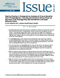
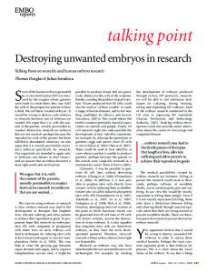
Wind Noise Model The noise model for wind is that of a nonstationary noise source with the energy concentrated in the lower frequencies and rolling off at approximately

as the

frequency increases [10,11]. The nonstationarity occurs because the bursts of wind are statistically dynamic and unpredictable. This causes subtractive filtering, Wiener filtering, and previous methods of noise reduction that assume stationary or quasistationary noise to perform poorly.

5 0 -10

Magnitude (dB)

-20 -30 -40 -50 -60 -70 -80 -90 0

1000

2000

3000 4000 5000 Frequency (Hz)

6000

7000

8000

Frequency

Figure 1: Power Spectral Density of Wind Noise

8000

40

7000

30

6000

20

5000

10

4000

0

3000

-10

2000

-20

1000

-30

0

0.5

1

1.5

2 Time

2.5

3

Figure 2: Spectrogram of Typical Wind Noise Bursts

3.5

6 Proposed Filter Model The filter model proposed takes advantage of the characteristics of the speech and noise for speech enhancement and noise suppression. The model is divided into two primary components, one for high frequencies (>4 kHz) and one for low frequencies (<4 kHz). The high-frequency module is a highpass filter. As shown in the wind models, even with very loud wind bursts, only a small amount of noise energy is in the higher frequencies. Since the speech signal typically dominates noise in the higher frequencies, a highpass filter works well for the frequencies 4 kHz and above. For the lower frequencies, the SNR is often lower than 0 dB. The filter model takes advantage of the fact that the majority of low-frequency content in speech is harmonic in nature. A coherent modulation comb filter is used to extract the harmonics from the signal. These harmonic signals contain both the energy of the speech and the noise at the harmonic intervals, but in the harmonics the speech has a much higher SNR than the original signal because the noise’s energy is spread more evenly throughout the spectrum while the speech’s energy is concentrated at the harmonics. The noise’s energy at the harmonics, however, is slight enough so that listenability increases after filtering within the range of typical wind noise SNR’s.

The filtering method as it is so far described works well in clean speech and in speech with wind noise. In the case of wind noise without speech, however, the method causes undesired artifacts because the comb filter transforms the broadband noise into a harmonic signal. This type of artifact is undesirable for two reasons. The first is that it is a foreign sound which can be distracting for the listener. Even though the unfiltered wind noise can be significantly louder, it is a familiar sound that people instantly identify. Such known noises are typically less distracting to a listener than unfamiliar sounds. The second reason why the artifact is undesirable is that intelligibility may be decreased if harmonic sounds are present if no speech is present. The best case, then, would be to attenuate the signal when there is wind noise present with no voiced speech,

7 an idea employed by Lim et al. [12]. This both reduces artifacts of processing and preserves the natural envelope of the clean speech.

Table 1: The optimal type of processing for combinations of speech and noise Noise Absent Noise Present Voiced Speech

No Filtering

Filtering

Unvoiced/No Speech

No Filtering

Attenuate Low Frequencies

2.2 RELEVANT PRIOR WORK Fundamental Tracking Using Least Squares Harmonic In order for coherent modulation filtering to work well, an accurate and robust fundamental frequency tracker is essential. There have been several algorithms proposed through the years, including comb filtering [13], autocorrelation analysis [14,15] instantaneous frequency estimation [16], center-of-gravity (COG) estimation [17], STRAIGHT [18,19], and least squares harmonic (LSH) model [20]. For the given application, the most important characteristics were pitch accuracy and robustness to noise. Since it would have been impractical to implement and test every popular algorithm for the given application, three methods were implemented and compared, COG, STRAIGHT and LSH. Initial work was done with the COG because it has frequently been used in conjunction with coherent modulation for carrier estimation. The main idea of the COG is to analyze a subband or broadband signal over a short window. Next, compute the discrete Fourier Transform (DFT) of the window. Finally, the first-order spectral moment is computed using the magnitude of the DFT: (2)

The frequency found from the center-of-gravity estimate is then taken to be the instantaneous frequency of the window. After some analysis, the COG was abandoned due to some undesirable properties for the task at hand. First of all, the COG has always

8 been used in fixed subbands, which presents several problems. The COG will calculate a carrier signal for each subband. This approach doesn’t take advantage of the harmonicity present in voiced speech because each subband is treated as independent. Also, rarely is a single harmonic present in each subband. The question of what to do when a subband has no harmonics or multiple harmonics is an unanswered question. Also, the COG estimate is biased due to the shape of the main lobe and the energy in the side lobes. Although a solution has recently been found in getting around the bias issue [21], the issue of multiple or no harmonics in a subband still presents problems. Another issue of the COG is that it doesn’t perform well in low SNR’s. This is because each subband is analyzed independently of the others, so the integer multiple harmonic relationships are not used advantageously.

Next, the STRAIGHT algorithm was analyzed. Although STRAIGHT works quite well for clean speech, it currently falls apart when any significant (0 dB SNR or lower) wind noise is present. LSH, however, can still track frequencies in much higher noise (-15 dB). Because LSH performed so much better than STRAIGHT, the LSH model was selected as the best pitch estimator for use in the wind noise removal system.

The LSH uses the Harmonic plus Noise model (H+N), where a signal can be decomposed into a quasi-periodic part (harmonic component) and an aperiodic part (noise component). This model is derived from the traditional speech model [9] where the vocal cords produce a quasi-periodic pulse train shaped by a linear time-varying filter consisting of the vocal tract, vocal cavities, and mouth. Thus, the harmonic component of the H+N model is the voiced part of the speech, and the noise component is the unvoiced speech as well as any other type of noise in the signal. If short enough temporal windows are used, such as 50 ms, the harmonic part of the speech can be assumed to have a constant frequency. Li et al. [22] have since extended the original LSH model to allow for linear, quadratic, and higher order fundamental frequency motion in a frame. With such freedom, longer frame sizes can be used because the

9 estimated carrier can better track the actual carrier’s motion. Higher order estimations, however, can take much longer to calculate, so the original method with a short 50 ms frame size was chosen as a good compromise between algorithm speed and accuracy. The H+N model with a stationary fundamental frequency represents a frame as a sum of a harmonic component

and inharmonic noise component

:

(3)

The harmonic component can be expressed as:

(4)

The mean square error (MSE) between

and

is:

(5)

For a given frequency, the minimum MSE is found by setting the two partial derivatives to zero and solving for and : (6)

10 In short, the LSH pitch tracking method therefore consists of the following steps: 1. Define a frequency range for calculating MSE’s 2. Calculate

and

for each frequency by solving minimum MSE

3. Find the frequency that provided the smallest MSE and designate it as the fundamental frequency for the frame 4. Move to the next frame and repeat The fundamentals of LSH presented here are based on concepts detailed in AbuShikkah et al. [20].

Comb Filtering Since its inception, comb filtering has been applied to a variety of speech enhancement problems. The two main types of comb filtering are FIR and IIR. FIR comb filtering for speech enhancement was explored by Shields [23] and Frazier et al. [24,25]. FIR comb filters enhance the periodic nature of a signal by placing evenly spaced filter coefficients at the supposed pitch period and setting all other coefficients to zero. This works on the principle of a moving average filter because it outputs the average waveform of several periods. Since the noise is assumed to be aperiodic, this attenuates the noise. This would work well if the speech were exactly periodic, but speech is better described as quasiperiodic because both the speech’s frequency and harmonic content can change, both of which will cause distortion in the FIR method. Due to the temporal blurring caused by comb filtering the quasiperiodic speech, this method decreases intelligibility despite its reduction of perceived noise [12,26].

11 2

0.25

1.5

0.2 0.15

1 Imaginary Part

Imaginary Part

0.1 0.5 480

0 -0.5

0.05 0 -0.05 -0.1

-1

-0.15 -1.5 -2

-0.2 -1

0 Real Part

1

0.85 0.9 0.95 1 1.05 Real Part

Figure 3: Pole/Zero Plot of FIR Comb Filter 10 0 -10

Magnitude (dB)

-20 -30 -40 -50 -60 -70 -80 -90 0

0.2 0.4 0.6 0.8 Normalized Frequency (×π rad/sec)

Figure 4: Frequency Response Curve of FIR Comb Filter

1

12 The other method, IIR comb filtering, was later developed by Nehorai and Porat [27] and improves upon many of the undesirable characteristics of the FIR comb filter. The method cascades a series of identical second-order IIR bandpass filters, with the number of cascaded filters corresponding directly to the number of harmonics in the comb filter. This method is advantageous compared to the FIR method in several ways. The first is computationally, as the FIR filter typically uses many more coefficients to obtain a magnitude frequency response than the IIR version. Secondly, it is simpler to tune the frequency response of an IIR comb filter because it is made up of several simpler bandpass filters. The FIR filter’s parameters, which are the filter length and coefficient weights, are less direct in indicating how they will affect the comb filter’s frequency response. The IIR’s parameters, which are the pole magnitude, zero magnitude, and number of filters cascaded, each directly relate to the filter’s passband gain, transition bandwidth, and number of harmonics to filter, respectively. A third advantage is a combination of the previous two, which is the fact that the IIR filter doesn’t suffer the same kind of temporal blurring that the moving-average characteristics of the FIR comb filter cause. This is because the IIR filter uses fewer coefficients.

Despite the significant advantages that the IIR comb filter has over its FIR counterpart, oftentimes high-order IIR comb filters are infeasible due to instability constraints, which can be seen in Figure 7. For example, an IIR filter containing fifteen harmonics becomes unstable below approximately 225 Hz (for fs=16 KHz), which is in the middle of the frequency range for female speech and about an octave above male speech. At lower sampling rates, the issue is even greater because the fundamental frequency at the stability boundary scales with the sampling frequency. For example, the fifteenharmonic (30th order) filter mentioned above becomes unstable at only 125 Hz for sampling rates of 8 kHz. This means that such a filter would be impractical for many speech applications.

13 The reason why high-order IIR filters have instability issues is because of quantization error on the filter coefficients. High-order IIR filters become extremely sensitive to this, with just a small quantization error causing a pole to jump outside the unit circle, making the filter unstable. In the work presented here, 64-bit doubleprecision numbers were used. In hardware systems, such as mobile devices, where 32bit or smaller words sizes are used, stability constraints are even more of an issue. In the following section we will present how coherent demodulation sidesteps these constraints to allow for IIR comb filters of arbitrary order (see Figure 8).

2 0.082 1.5 0.081 Imaginary Part

Imaginary Part

1 0.5 0 -0.5

0.08 0.079 0.078 0.077

-1 0.076 -1.5 0.075 -2

-1

0 Real Part

1

Figure 5: Pole/Zero Plot of IIR Comb Filter

0.9950.9960.9970.998 Real Part

14 0 -5

Magnitude (dB)

-10 -15 -20 -25 -30 -35 0

0.05 0.1 0.15 Normalized Frequency (×π rad/sec)

0.2

Figure 6: Frequency Response Curve of IIR Notch Comb Filter Stable = Green, Unstable = Red

Fundamental Frequency (fs = 16kHz)

300

250

200

150

100

50 0

5 10 15 20 Number of Harmonics (Filter Order is Twice the Harmonic Order)

Figure 7: Normal IIR Comb Filter Stability

15 Stable = Green, Unstable = Red

Fundamental Frequency (fs = 16kHz)

300

250

200

150

100

50 0

5 10 15 20 Number of Harmonics (Filter Order is Twice the Harmonic Order)

Figure 8: Coherent Modulation Comb Filter Stability Coherent Modulation Filtering Coherent demodulation has been developed in the last few years as a new way of representing a signal as a set of carriers and modulators. It had been spawned as a reaction to some of the shortcomings of incoherent modulation filtering [28] that uses the Hilbert transform

to break a signal into an envelope

and carrier

: (7) (8) (9)

The k's in the above and following equations denote that signals may be divided into a set of bandlimited analytic signals using subbands or other methods if desired. Some of the shortcomings of incoherent demodulation are that the bandwidth of the Hilbert

16 carrier is typically larger than that of the original analytic signal [29]. Also, filtering the envelope introduces significant artifacts. Atlas et al. [30] have proposed that the reason that the Hilbert transform is incorrect is because of its assumption that the envelope be nonnegative and real. By not restricting the modulator to be nonnegative and real, both the carrier and modulator enjoy better characteristics, such as a reduced-bandwidth carrier and artifact-free modulation filtering. In order to distinguish the two, the term “incoherent modulation” has been applied to the Hilbert transform and “coherent modulation” has been applied to the new method where the modulator need not be nonnegative and real.

Coherent demodulation is similar to the incoherent approach in that they both break up an analytic signal into a single carrier/modulator product pair. The difference, however, is how the carrier and modulator are estimated. The incoherent approach simply splits a signal into a magnitude and phase component, which are the modulator and carrier. The coherent approach, in contrast, first estimates the carrier of the signal (LSH is used in this work, but carrier estimators may be used) and then multiplies the signal by the carrier's complex conjugate to determine the modulator:

(10)

The analytic signal of a subband is represented as: (11)

In order to calculate the modulator, the signal is multiplied by the complex conjugate of the carrier: (12)

17 After the modulator is isolated, it may be filtered as desired. To recapitulate, coherent modulation filtering consists of splitting a signal into a series of carriers (with or without the use of subbands), finding the coherent modulator for each carrier, filtering the modulator, recombining the filtered modulator with the original carrier, and adding the signals back together. So far, coherent modulation filtering has been applied to speech enhancement [31-33] and musical instrument separation [34] by Atlas et al. Most of the research in this area to date has used simple linear time-invariant FIR filtering on the modulator. In this case, the modulators can be thought of in another way. A lowpass modulation filter can also be considered a time-varying bandpass filter with a fixed bandwidth and a center frequency that tracks the estimated carrier frequency found by the desired carrier tracking method. The new method proposed here, coherent modulation comb filtering, modulates an adaptive comb filter so that it can filter any desired consecutive harmonics, such as harmonics six through ten, something which has not been possible before with traditional comb filters. A much more detailed description of coherent modulation comb filtering will be presented later in the text.

In conclusion, incoherent demodulation is not without its uses. The Hilbert envelope can be useful in displaying the temporal evolution of a signal’s energy or other analysis applications, but incoherent modulation filtering as proposed by Drullman et al. [35] introduces such significant artifacts that it likely will not have practical use in the future and will be replaced by its successor, coherent modulation filtering.

18 CHAPTER 3: WIND NOISE REMOVAL ALGORITHM THEORY, IMPLEMENTATION, AND RESULTS

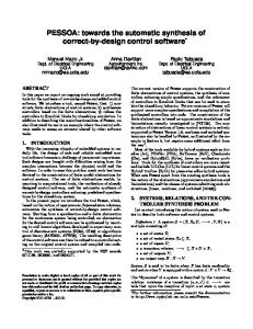
3.1 OVERVIEW Algorithm First, a high-level description of the wind noise removal algorithm will be presented. The first component of interest is the fundamental tracker, which computes a pitch estimate for each frame using LSH and an error term which represents the harmonicity of the input signal. The error term is used by the wind detector to decide whether or not wind is present. The time-varying pitch estimation is used to demodulate the original signal by integer multiples of

. These demodulated signals are then filtered by comb

filters constructed to follow the fundamental trajectory. After filtering, these signals are remodulated to their original frequencies. These are added together to construct the harmonic segment of the signal. The gain on this signal is adjusted according to the conditions of the signal frames. If the frame contains wind without voiced speech, the signal is muted. If there is no noise in the signal, no gain is applied. A highpass filtered version of the original signal added to the coherent modulation comb filtered components comprises the output of the system.

19 x(n)

V/UV Detector

Highpass Filter

Automatic Gain Control

v/uv Index

Wind Detector

Gain Factor

Wind Index

Error

x(n)

Fundamental Tracker

5-Harmonic Comb Filter

f0

Coherent Demodulator (5f0)

5-Harmonic Comb Filter

Coherent Modulator (5f0)

+

Coherent Demodulator (10f0)

5-Harmonic Comb Filter

Coherent Modulator (10f0)

+

Coherent Demodulator (5nf0)

Nmod5Harmonic Comb Filter

Coherent Modulator (5nf0)

+

x

+

y(n)

Figure 9: Block Diagram of N-Harmonic Wind Noise Removal Algorithm Test Data For testing, speech samples are used from Carnegie Mellon University’s ARCTIC database [36]. Samples include male and female speakers with American, Irish, and Indian accents ranging in length from 3 to 5 seconds. The wind samples were recorded outside a windy Seattle evening using a Roland Edirol R09 24-bit portable recorder. The wind recordings were then split up into 11 distinct wind bursts ranging in length from 0.33 to 1.25 seconds. Other than normalization, no other processing was done on the wind samples. A gain term was then applied to the wind burst to achieve a desired SNR before being added to a speech sample. In order to model the unpredictable nature of wind bursts, a Poisson distribution with a half-second mean was used to define the distance between wind bursts. This distribution was chosen as it roughly approximates

20 the frequency of gusts on a windy day. The wind bursts themselves were then chosen randomly from the set of samples. The second type of noise tested was steady speechshaped noise (SSN). This algorithm was not originally designed for use with SSN, but was included for testing because of an organization’s interest in removing this type of noise. The noise was then similarly added to the speech at various SNR’s. The SNR’s used for each case were 0 dB to -30 dB in 3 dB increments. In most situations, wind noise probably won’t reach -30 dB, but this large range was chosen in order to see the performance limits of the components.

3.2 VOICED/UNVOICED SPEECH DETECTOR Theory A voiced/unvoiced speech detector is desired to aid in controlling the envelope for the lower harmonic frequencies (<4 kHz). The three instances of noisy signals are noise with voiced speech, noise with unvoiced speech, and noise without speech. During voiced speech with noise, it may be most natural sounding to decrease the gain slightly to compensate for the extra energy introduced by the comb filtered harmonics. However, during unvoiced or no speech, it is best to completely attenuate the lower frequencies. If this does not occur, the sound resulting from wind noise being transformed by the comb filter into a harmonic signal via the comb filter is an undesirable, unnatural-sounding artifact. Also, the voiced/unvoiced detector is used by the fundamental frequency trajectory processor, as the trajectory interpolates through unvoiced parts of the signal. This is helpful because the pitch trajectory moves around rapidly during unvoiced parts, which can cause undesirable artifacts.

There has been much work in the task of voiced/unvoiced speech detection. A variety of methods have been used, including autocorrelation [14,15,37,38], classification [39,40], delta modulation [41], linear prediction coefficients (LPC) [37], and others. The method developed here uses autocorrelation. This was chosen because it is relatively simple and works fairly well. It is important to mention that although this component is important

21 in the whole wind noise removal algorithm, the new contribution and major research topic of the thesis is the coherent modulation comb filter. The detector implemented here uses many of the ideas seen in previous work in the subject and was meant to just get the initial wind noise removal algorithm up and running. The current setup can be divided into the following three steps: prewhitening, autocorrelation, and postprocessing.

Implementation Since the autocorrelation method works on the assumption that the speech is periodic, the same 50 ms frames with a 50% overlap are used as for the pitch tracker and wind noise detector. The first task uses low-order linear prediction error residuals [42] on a frame to prewhiten the signal. Not only does this aid in removing the formant structure, but also assists in increasing the SNR. Next, the autocorrelation of the processed frame truncated to about 3 pitch periods is calculated. Then, the five highest peaks of the autocorrelation are found. In the case where two peaks are very close to one another (less than 1.5 ms apart), only the highest peak in that segment can be picked. Next, the algorithm determines whether or not the 5 peaks are within range of being a proper pitch period. The pitch period range is determined from the hand-selected frequency ranges for each of the speech signals. If a peak falls within range, it then determines if at least one of the other peaks is an integer multiple of the pitch period, within an 8% tolerance. If the frame passes these conditions, it is marked as being voiced. Otherwise, the frame is marked as unvoiced. After the initial detector makes a decision on all the frames, these are then processed to reduce errors on difficult frames. Examples of difficult sounds are frames containing diphthongs or other transitions between two voiced phonemes. Also, since the purpose of the detector is to find longer (50 ms or greater) periods of noise during no speech or unvoiced speech so that they can be attenuated, it is desired that short consonants (such as the consonants in “taco”) be labeled as voiced to avoid unwanted attenuation. To achieve these goals, a short median

22 filter is used. The binary decisions for each of the frames are then ready to be used by the fundamental frequency tracker and automatic gain control components.

Results The two figures below show the unvoiced/voiced decisions for both speech in wind noise and speech in SSN. The red dashed line indicates a 50 ms frame or longer of unvoiced or no speech with a nonzero value. The algorithm starts to have problems identifying the voiced parts when the SNR exceeds about -9 SNR. Other times when the v/uv detector has errors are when the voiced speech is rapidly changing, such as at a transition between two vowels. In such cases, the autocorrelation method has problems because the waveforms of adjacent periods don’t line up well and thus do not have a high correlation at pitch period intervals.

8000 7000

Frequency

6000 5000 4000 3000 2000 1000 0

0.5

1

1.5

2 Time

2.5

3

3.5

Figure 10: V/UV Decisions on Speech with Wind (-9 dB SNR)

23 8000 7000

Frequency

6000 5000 4000 3000 2000 1000 0

0.5

1

1.5

2 Time

2.5

3

3.5

Figure 11: V/UV Decisions on Speech with SSN (-9 dB SNR) 3.3 FUNDAMENTAL TRACKER Theory A fundamental frequency tracker is one of the most important components because if the fundamental trajectory is incorrect, the comb filter will attenuate the true harmonics and instead boost the noise. The fundamental tracker developed has two stages. The first stage calculates an

estimate for each frame. The second stage processes these

estimates to smooth them over time and to interpolate through sections with a very low SNR or otherwise have a high likelihood of a poor estimate.

Implementation The first stage of the fundamental tracker is calculating pitch estimate for each frame. The frame size is 50 ms with a 50% overlap. These lengths were chosen because they are short enough for the assumption that the speech contained in a frame is periodic and the 50% overlap is a good tradeoff between time resolution and computation time. Input

24 parameters for the LSH algorithm are the frequency range and number of harmonics to use in the LSH calculation. The frequency range for LSH has so far been chosen by hand to encompass the speaker’s pitch range. In future work, however, autocorrelation or another method can be used to approximate a frequency range real-time. The other parameter was the number of harmonics to use, which was set to be 25. This also could be determined automatically in the future. Since the majority of voiced speech is in the lower frequencies and that the unvoiced speech is typically contained in the higher frequencies, the frames were low-pass filtered at 3 kHz to mitigate the interference of the unvoiced speech on LSH.

After the pitch estimates are calculated for each of the frames, the next stage is processing its trajectory to smooth the discrete steps between frames and to interpolate through segments that have very low SNR, that are varying too quickly to be natural speech, or that otherwise have a high likelihood of being incorrect. The first part uses the voiced/unvoiced information to label the unvoiced frames as having incorrect pitch estimates. This criterion is chosen for two reasons. First of all, in quiet sections of audio or in sections of unvoiced clean speech, the pitch estimates can vary quickly, which can cause unnatural artifacts in the final signal. Secondly, in voiced sections that are degraded by noise so significantly that it is labeled as unvoiced, the SNR is usually so low that the pitch estimate is also off target. In future implementations, the pitch tracker can skip such frames because the estimates calculated for these frames are not going to be used anyways. Next, the unvoiced frames are interpolated over with a linear interpolator. Finally, a moving average filter is used to smooth over the entire signal to remove the discrete steps found at the frame boundaries in order to get a more natural trajectory.

Results In order to test performance of the fundamental tracker, a nominal trajectory was calculated for each of the 8 speech signals by using LSH and the f0 processing on each

25 of the clean signals. They were then projected onto spectrograms and visually inspected to verify that they looked correct. Next, the fundamental trajectories were calculated for each of the speech samples with the specified SNR’s for the wind noise. The accuracy percentage was calculated by averaging the pitch accuracy over all the points containing wind:

(13)

Table 2: Mean Error Percentage from True Trajectory SNR (dB) Error in Wind (%) Error in SSWN (%)

0

-3

-6

-9

-12

-15

-18

-21

-24

-27

-30

2.29

2.62

2.94

3.60

4.21

4.96

5.28

5.61

6.06

6.35

6.12

2.04

2.01

2.11

2.35

2.53

2.25

2.81

3.41

4.53

6.61

10.35

The two figures below illustrate the performance of the two stages of the fundamental tracker. Figure 10 shows the pitch trajectory calculated directly from LSH. This figure also includes the paths of the first ten harmonics. This figure shows how there can be sharp transitions between frames. Also, during unvoiced parts of speech, the calculated pitch estimates have a high variance. Both of these can introduce artifacts and explain the need for post-processing the raw LSH estimate. Figure 11 shows the trajectory after the interpolation and smoothing. This trajectory looks more natural than the original and eliminates the artifacts plaguing the raw estimate.

26 3000

2500

Frequency

2000

1500

1000

500

0

0.5

1

1.5

2 Time

2.5

3

3.5

Figure 12: Fundamental Trajectory from LSH estimate (-9 dB SNR)

3000

2500

Frequency

2000

1500

1000

500

0

0.5

1

1.5

2 Time

2.5

3

3.5

Figure 13: Fundamental Trajectory after Processing (-9 dB SNR)

27 3.4 WIND DETECTOR Theory The wind detector is used to decide when wind noise is present in a signal. This information can be used in two ways. The first is in controlling the parameters of the filter. Although the comb filter has fixed pole and zero magnitudes in its current implementation, the wind detector in future implementations will provide information to control these parameters to “clamp down” when wind is present and then relax its filtering bandwidth or be bypassed completely during segments of insignificant noise. Another use of knowing whether wind is present is used by the post-filtering gain control, which attenuates the lower frequencies for frames where noise is present and voiced speech is absent.

The wind detector works on the premise that when there is a significant amount of inharmonic energy in the lower frequencies (below 4 kHz), wind or another type of broadband noise is present. The original signal and the MSE from the LSH fundamental tracker are used to calculate the inharmonic energy. Two error representations are used to compute the binary decision. Tests are performed with each error term, and the frame is labeled wind if both tests return positive for wind. The first test is the energy ratio between the error term and the original signal, called the noise-to-composite ratio (NCR), represented in dB. Since the error term can never be greater than the energy of the original signal, the NCR is strictly non-positive. If the NCR is low (large negative number in dB), this means that the majority of the frame’s signal is harmonic. Conversely, if the NCR is high (close to 0 dB), this means that the frame contained mostly broadband energy in the form of noise or unvoiced speech. A threshold is used to make a hard decision, meaning that if the NCR is above a certain value, it is labeled as possible wind, and is labeled as not wind if it isn’t. The first test performs well when energy is present in the signal, but returns a false positive at quiet intervals when neither speech nor noise is present. In this case, the NCR is above the threshold because the

28 original signal is also quite low even though the error term is small. In order to account for these situations, a threshold is also applied to the MSE. A low MSE results in a negative decision and a high MSE results in a positive wind decision. It is important to mention that other metrics could have been used for this secondary test. A power threshold on the original signal would have worked as well.

If both tests pass for a frame, the frame is labeled as containing wind. This “raw” decision is compared with neighboring frames and processed to remove likely false positives and better cover the onsets and offsets of wind bursts. The details of these two tests and processing are in the next section.

Implementation The first stage of the wind detector calculates a raw frame-by-frame decision based on the NCR and MSE of each frame. The threshold of the NCR is set at -2 dB, which provides a favorable sensitivity to wind noise. The threshold for the MSE is set to be the mean MSE of all the frames. In a practical implementation, this threshold could likely just be set to just above the noise floor of the microphone or another particular value, but since the current implementation was developed in Matlab and can effectively scale the signal in several ways, the mean MSE was instead used.

After the raw wind frame decisions for each of the tests are calculated, these decisions are processed to better encompass wind onsets and offsets and to allow for filtering to “clamp down” in later implementations, as well as remove likely false positives. First, the test results are processed individually. For each index with a positive detection, the three preceding and the three following frames are marked as positive, which adds the buffer intended to encompass the onsets and offsets of the wind as well as the transition times for a filter to clamp down. Next, the two sets of processed wind decisions are combined together point-by-point with a logical AND, meaning that the resulting frame is positive if both the input frames from the CNR and MSE tests are positive. This new

29 wind index, however, may contain short gaps in what should be a series of consecutive positive or negative indices. In order to correct for this, a median filterbased method is used that marks a frame positive if the previous frame is positive and at least one of the following two frames are positive. Otherwise the frame is marked negative. More research could be done in wind detection in the future, but the current implementation is a good starting point for further work.

Results Testing has shown that the wind detector works satisfactorily at high SNR’s and quickly increases in accuracy as the SNR drops. This is intuitive because it makes sense that it would be easier to detect louder noises than quieter noises. At medium levels of wind noise (-6 to -9 dB SNR) the error is less than 2%. These errors also typically occur at the onsets and offsets of wind, as can be seen below in Figure 12, in which the magenta lines represent the endpoints of the actual wind noise clips and the white lines represent the decision from the wind detector. For example, a false negative is occurring during the end of the second burst below. The wind noise is actually present until about 3.1 seconds, but since the energy is so much lower than the peak wind noise levels, it is classified as not being wind. The figure below the spectrogram shows how the CNR and MSE vary over the signal as well as their threshold. In practice, the wind detector will likely work even better because the MSE threshold will be set to be a constant or dynamically change over time, while in the current implementation it is simply the mean of the short audio clip. Table 3: Wind Detector Performance SNR (dB) False Neg. (%) False Pos. (%) Total Error (%)

0 7.64 5.36 12.99

-3 3.94 2.76 6.70

-6 2.51 1.00 3.50

-9 1.48 0.28 1.76

-12 1.02 0.05 1.08

-15 1.00 0.00 1.00

-18 1.00 0.00 1.00

-21 1.03 0.00 1.03

-24 1.03 0.00 1.03

-27 0.99 0.00 0.99

-30 0.97 0.00 0.97

30 8000 7000

Frequency

6000 5000 4000 3000 2000 1000 0

0.5

1

1.5

2 Time

2.5

3

3.5

Figure 14: Wind Detector Decisions for a Windy Signal (-9 dB SNR). Note that the magenta denotes the actual wind noise clips and the white denotes the periods labeled as wind by the detector.

31 Noise to Composite Ratio (dB) 0

-5

-10

0.5

1

1.5

2

2.5

3

3.5

3

3.5

Mean Square Error 0.06 0.04 0.02 0

0.5

1

1.5

2

2.5

Figure 15: NCR and MSE Measurements for a Windy Signal (-9 dB SNR) 3.5 COHERENT MODULATION COMB FILTER Theory The coherent modulation comb filter uses coherent demodulation techniques to extend the capabilities of a traditional IIR comb filter. Since the pitch of speech is time-varying, the time signal is divided into short frames where the pitch is assumed constant. In each frame, the signal model is a summation of a harmonic component inharmonic component

and an

, which is similar to the H+N model used by the LSH pitch

tracker except that the modulator can be time-varying:

(14)

32 The goal is to remove the inharmonic component and keep the harmonic component. To do this, a notch filter

is created and then subtracted from the original signal in

order to emphasize the harmonics: (15)

Where

is the DC gain of the filter. The comb filter is created by cascading a series of

identical bandpass filters together:

(16)

where (17) The parameter is the magnitude of the poles [27]. As the magnitude approaches 1, the bandwidth of the filter tightens around the defined harmonics. The filter outlined above becomes unstable for certain frequencies when the harmonic count exceeds 5, thus introducing the need for a new method of comb filtering.

Coherent modulation comb filtering extends the stability constraints of traditional IIR comb filters to allow filtering of any number of harmonics. By coherently demodulating the original signal, normal comb filters can be used to filter up to five consecutive harmonics anywhere in the signal. As an example, the following steps are used to filter harmonics

through

:

1. Compute the analytic signal of the real-valued signal:

33 (18)

2. Demodulate the signal by

. This centers the harmonics of interest around

DC. 3. Lowpass filter signal by the range of harmonics

. This filters out all frequency content outside through

4. Modulate the signal by through

. to lines up to the harmonic positions into

.

5. Use a normal 5-harmonic time-varying comb filter on the signal. 6. Remodulate signal by

to return harmonics to original frequencies.

The above algorithm can be used to filter any number of harmonics desired.

3000

2000

Frequency

1000

0

-1000

-2000

-3000

0.2

0.4

0.6

0.8

1 1.2 Time

1.4

Figure 16: Step 1 – Compute the Analytic Signal

1.6

1.8

34 3000

2000

Frequency

1000

0

-1000

-2000

-3000

0.2

0.4

0.6

0.8

1 1.2 Time

1.4

1.6

1.8

1 1.2 Time

1.4

1.6

1.8

Figure 17: Step 2 – Demodulate

3000

2000

Frequency

1000

0

-1000

-2000

-3000

0.2

0.4

0.6

0.8

Figure 18: Step 3 – Lowpass filter

35 3000

2000

Frequency

1000

0

-1000

-2000

-3000

0.2

0.4

0.6

0.8

1 1.2 Time

1.4

1.6

1.8

1.6

1.8

Figure 19: Step 4 – Modulate for Comb Filter

3000

2000

Frequency

1000

0

-1000

-2000

-3000

0.2

0.4

0.6

0.8

Figure 20: Step 5 – Comb Filter

1 1.2 Time

1.4

36 3000

2000

Frequency

1000

0

-1000

-2000

-3000

0.2

0.4

0.6

0.8

1 1.2 Time

1.4

1.6

1.8

Figure 21: Step 6 – Remodulate Harmonics to Original Frequencies Implementation In the current implementation, the exact same comb filter is used for filtering each of the sets of harmonics. Future work will include looking into having a tight bandwidth at lower frequencies and relax it as the as the frequency increases. This would likely decrease audible artifacts by allowing for a smoother transition to the highpassed frequency component. Currently, however, a pole magnitude of 0.999 is used, which provides about 30 dB of stopband attenuation.

Results In order to compare the listenability of the unprocessed, normal comb filter, and coherent modulation comb filter, a test program based on [43] was given informally to 7 subjects with normal hearing. The GUI used was:

37

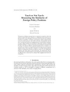
Figure 22: Test GUI The listener rated the listenability of the unprocessed reference signal to the test signal. The test signals were made up of 2 speech clips (male/female) x 2 noise types (wind noise/speech-shaped noise) x 4 SNR’s (-6/-12/-18/-24dB) x 3 test signals (unprocessed/normal comb filter/coherent modulation comb filter) x 4 repetitions of each signal, totaling 192 examples. The graph below shows the results of the tests:

Female Speech in SSWN

Quality

Female Speech in Wind Noise 10 9 8 7 6 5 4 3 2 1 -6 -12 -18 -24 SNR (dB) Male Speech in Wind Noise 10 9 8 7 6 5 4 3 2 1 -6 -12 -18 -24 SNR (dB)

Quality

Quality

Quality

38

10 9 8 7 6 5 4 3 2 1

10 9 8 7 6 5 4 3 2 1

Black: Unprocessed Red: Regular Comb Filter Green: CMCF

-6

-12 -18 -24 SNR (dB) Male Speech in SSWN

-6

-12 -18 -24 SNR (dB)

Figure 23: Informal Listening Test Results Although the coherent modulation filtering is either on par with or outperformed by the comb filter, these results give valuable insight into listener preferences. For female speech in wind noise, the processing with the normal comb filter and CMCF output similar sounds, resulting in a similar score. This is because the vast majority of the wind energy is below the fifth harmonic. In comparing the three figures below, it is apparent that a small amount of wind is left over in the higher harmonics, but not enough to significantly bother most listeners. In samples of male speech in wind noise, the normal comb filter scored significantly higher in all cases. A reason why this may have happened is since the harmonics in male speech are closer together, more wind noise is able to get through the comb filters in the form of “harmonicized” noise. This noise sounds unnatural and causes listeners to score it poorly. In the normal comb filtering examples, the comb filter still produces harmonic noise. But since the highpass filter

39 frequency is about half that of the female speech, a significant amount of unprocessed wind noise makes it through in the highpass filtered part. It is hypothesized that this familiar wind noise perceptually masks the unnatural harmonic noise, thus leading to a more preferable sound than the CMCF that has filtered all the wind noise’s entire frequency range. 8000

30

7000

20

Frequency

6000

10

5000 0 4000 -10 3000 -20

2000

-30

1000 0

0.5

1

1.5

2 Time

2.5

3

3.5

Figure 24: Female Speech with Wind Noise (-6 db SNR)

-40

40 8000

30

7000

20

Frequency

6000

10

5000 0 4000 -10 3000 -20

2000

-30

1000 0

0.5

1

1.5

2 Time

2.5

3

3.5

-40

Figure 25: Female Speech with Wind Noise (Normal Comb Filter)

8000

30

7000

20

Frequency

6000

10

5000 0 4000 -10 3000 -20

2000

-30

1000 0

0.5

1

1.5

2 Time

2.5

3

Figure 26: Female Speech with Wind Noise (CMCF)

3.5

-40

41 The female voice in speech-shaped noise seemed to boil down to the listener’s preference of noise. The unprocessed noise’s energy is concentrated in the lower frequencies. The processed signals removed the lower frequency component of the noise, both reducing the SNR and changing the color of the noise. Many people commented on how they preferred the unprocessed noise to the quieter, but perceptually harsher, noise. For the samples of male speech in colored noise, the coherent modulation filter scored lower than the regular comb filter. In addition to the color preferences of the unprocessed versus processed noise and the presence of a hard edge in frequency, another reason may be due to the poor SNR in the upper harmonics. In the coherent comb filtered sample (Figure 28), the speech signal can be clearly seen in the first five harmonics. In the higher harmonics, however, the noise begins to dominate. This causes the tone of the voice to sound more unnatural. The primary conclusion from these results is that many people prefer a signal with fewer artifacts and more noise than vice-versa. In the future, more work will be done to optimize the tradeoff between the two.

42 8000

30

7000

20

Frequency

6000

10

5000 0 4000 -10 3000 -20

2000

-30

1000 0

1

2

3

4

-40

Time

Figure 27: Male Speech with Speech-Shaped Noise (-24 db SNR)

8000

30

7000

20

Frequency

6000

10

5000 0 4000 -10 3000 -20

2000

-30

1000 0

1

2

3

4

-40

Time

Figure 28: Male Speech with Speech-Shaped Noise (Normal Comb Filter)

43

8000

30

7000

20

Frequency

6000

10

5000 0 4000 -10 3000 -20

2000

-30

1000 0

1

2

3

4

Time

Figure 29: Male Speech with Speech-Shaped Noise (CMCF)

-40

44 CHAPTER 4: CONCLUSIONS AND FUTURE WORK

4.1 CONCLUSIONS Through this work, several conclusions have been reached. The most important conclusion and central point of the thesis is that coherent modulation comb filtering successfully lifts the stability constraints of regular IIR comb filters. Other key conclusions are discussed below.

Listener Perception The results from the listening tests showed that the regular comb filter was scored higher than the CMCF. There are a few hypotheses why this difference occurred. The first relates to the speech in colored noise. In the higher harmonics, the noise energy typically dominates the speech energy. This causes the filtered signal to contain harmonic energies inconstant with speech, making the voice sound unnatural. Also, there is a sharp transition between the low and high frequencies, which also causes artifacts. To alleviate this, two changes are needed. The first is to have a less sharp transition band for the highpass filter. The second is to increase the bandwidth of higher harmonics. This bandwidth increase is also helpful in order to allow the comb filter to allow some frequency variation in harmonics as well as errors in the pitch estimate. In the current implementation, the bandwidths for all the harmonics are fixed. In the future, work should be done in determining the best way for bandwidth expansion, such as linearly, logarithmically, or based on hearing models. Speech enhancement in wind noise will also benefit from such a bandwidth expansion function by decreasing artifacts.

Testing Regarding testing, there are also some conclusions. The first is that listenability is a complex metric because it relies on many factors, including perceived noise, artifacts, volume levels, and listener preferences. The volume level is important because listening

45 to wind noise at low volumes is less fatiguing than at higher volumes. Since the listeners were able to choose a comfortable volume for themselves instead of fixing it for all the tests, the differences in volume likely affected the listener’s scores. Another factor, listener preferences, point to the fact that some listeners may prefer more noise and fewer artifacts while others prefer less noise and more artifacts. Another important point to mention is that the perceived performance of the wind noise removal system depends highly on the timing of wind and speech. In future testing, more samples of audio with different samples of wind at different times will help to average this out. Finally, it will be important to conduct a more formalized listening test for more accurate results.

4.2 FUTURE WORK This work presents an introductory exploration of CMCF for speech enhancement and has established a foundation for many future research topics, which are presented below.

Adaptive Coherent Modulation Comb Filtering Development Currently, the comb filter is always “turned on”, meaning that it is always filtering the signal regardless of the signal’s SNR. One of the next steps in research will be to make the pole and zero magnitudes time-varying. This will allow the filter to “clamp down” and filter during lower SNR’s and “let up” during segments of less noisy speech. Also, further planning has to be done to decide how to best control the comb filter’s bandwidth. For example, whether the bandwidth values should be two discrete values or consist of a smoother range. Also, it would be desirable to be able to provide system with a single parameter controlling bandwidth to allow a user to choose an optimal point for the noise-artifact tradeoff. Implementing these ideas is will be important in transitioning the proposed system from a research project into a real-world application.

46 Speech Enhancement for Unvoiced Speech In the basic speech model [9], speech is categorized as voiced or unvoiced. Currently, the filtering algorithm presented focuses on the voiced part of speech by enhancing its harmonics. Except for simple LTI filtering, nothing is being done to enhance the unvoiced parts of speech currently. The reason why the voiced speech enhancement was developed first is because the majority of wind noise’s energy is in the lower frequencies where the voiced speech resides. Therefore, the current implementation works well for wind noise but doesn’t perform as well when the higher frequencies are more significantly degraded by noise as was seen in the SSN. In order to extend the algorithm’s robustness to other noise scenarios, researching unvoiced speech enhancement will be necessary.

Comparison/Integration with other Methods There has already been a significant amount of work on wind noise attenuation and even more on general speech enhancement. One area of future work will be to conduct a more thorough investigation of previous methods, compare them with the method proposed here, and most importantly see if any of the methods could be used in conjunction with CMCF to outperform the algorithms used separately. Some existing methods that look promising are Nonnegative Sparse Coding (NNSC) [3] and Nonnegative Matrix Factorization (NMF) [44,45].

Clipping For initial work, care was taken to make sure that no clipping occurred in the examples. Depending on the hardware configuration and recording conditions, however, clipping may be a possibility. Due to the nonlinear distortion caused by clipping, it is unknown how CMCF will perform in such circumstances. It is possible that the algorithm may perform just as well for clipped audio or attenuate its effects. However, it may degrade the performance of the fundamental tracker, voiced/unvoiced speech detector, or other components. Some work has been done in clip restoration [46,47] that might be useful

47 to preprocess the signal when clipping is detected. These possibilities should be explored in the future.

Fundamental Tracking Since the performance of the pitch tracker and the quality of the final signal are so closely related, an accurate, robust fundamental frequency tracker is essential. Future work on this component include further comparison with currently existing methods, preprocessing the signal for better tracking, and speeding up the algorithm. Since the focus of this thesis is on CMCF, much more work was done on its development than on pitch estimation. The LSH tracker was chosen because it performed well in low SNR’s. However, there may be other trackers that work even better in lower SNR’s or work comparably but with less computation time, so more work should be done in this area before developing this system into a real-world application.

One idea that has potential is combining coherent demodulation with LSH. The current problem with traditional pitch trackers is that small errors in frequency are multiplied in the higher harmonics. For example, a 1 Hz error in tracking the fundamental results in a 20 Hz error for the 20th harmonic. Such an error will cause a comb filter with a tight bandwidth to completely filter out the correct harmonic. To get around this problem, higher-order harmonics can be downshifter via coherent demodulation and then be used with a traditional pitch estimator. This could potentially significantly improve pitch estimation in the higher harmonics. A question that arises is what to do if the pitch estimates for the higher and lower harmonics aren’t in agreement. In that case, the best idea would probably be to either choose the estimate closest to the previous frame’s value or to choose the estimate with the lowest noise by comparing CNR’s.

Once a pitch tracking algorithm has been chosen, work should be done to decrease processing latency. One idea is to simply turn off the algorithm when no wind is detected. Currently, the wind detector uses information from the fundamental tracker, so

48 some nontrivial modifications would be necessary to the setup. Also, since the LSH algorithm is non-convex, the algorithm computes the fundamental frequency by performing an exhaustive search through the search space. Therefore, computation time can be greatly reduced by decreasing this space. One idea is to use autocorrelation [14,15,38] or other less computationally expensive methods to obtain a fast initial estimate which LSH can use as a starting point for your estimations. Another method is to first estimate the fundamental using big steps in frequency, then “zoom in” to a smaller range with finer resolution, and repeat until desired resolution is achieved. The two methods proposed here are complimentary and may be used in conjunction with one another. The final idea, which is purely developmental as well, is that the CMCF can take advantage of parallel processing because each piece is being filtered independently, which may be advantageous depending on the specifications of the system.

V/UV Detection Another area of future work includes further research in voiced/unvoiced speech detection. The detector here was developed quickly so that work could remain focused on the central research topic of CMCF, but in order for the automatic wind noise removal algorithm to transition from research into a real-world application, further research and development is necessary. It is possible that one or more existing detectors [14,15,38,37,40,39,41] would work well in wind noise, so these should first be examined before a whole new approach is developed.

Testing Finally, more testing is necessary in order for better performance evaluation and comparison with other methods. So far, only informal listening tests been conducted, but in the future, formal listening tests with more samples will be essential. Both listenability and intelligibility are important metrics to test. In addition to the wind noise bursts and SSN tested here, it would also be insightful to test other types of noise to see

49 if CMCF proves useful, such as babble talk, water (e.g. waterfall, fountain) sounds, or other background noise. Also, it will be important to test examples with different characteristics, such as samples with prominent room acoustics, far-field speakers, and speech recorded in the presence of noise instead of mixing clean speech and noise in the studio. Another potential use of the coherent modulation comb filtering is as a preprocessor for automatic speech recognition (ASR) systems. Since the wind noise removal system proposed here significantly increases the SNR in wind noise, it is possible that preprocessing the speech signal might increase accuracy in noisy scenarios where ASR currently performs poorly. Thus, future work should be done to verify whether or not coherent modulation comb filtering is an effective preprocessor.

50 REFERENCES

[1] N. Wiener, Extrapolation, Interpolation, and Smoothing of Stationary Time Series, The MIT Press, 1964. [2] S. Boll, “Suppression of acoustic noise in speech using spectral subtraction,” IEEE Transactions on Signal Processing, vol. 27, 1979, pp. 113-120. [3] M. Schmidt, J. Larsen, and Fu-Tien Hsiao, “Wind Noise Reduction using NonNegative Sparse Coding,” Machine Learning for Signal Processing, 2007 IEEE Workshop on, 2007, pp. 431-436. [4] S.T. Roweis, “One Microphone Source Separation,” NIPS, 2000, pp. 793-799. [5] D. Ellis and R. Weiss, “Model-Based Monaural Source Separation Using a VectorQuantized Phase-Vocoder Representation,” Acoustics, Speech, and Signal Processing. ICASSP 2006 Proceedings, 2006, p. V. [6] S. Roweis, “Factorial models and refiltering for speech separation and denoising,” 2003. [7] R. Weiss and D. Ellis, “Estimating Single-Channel Source Separation Masks: Relevance Vector Machine Classifiers vs. Pitch-Based Masking,” Pittsburgh, PA: 2006. [8] M. Schmidt and R. Olsson, “Single-channel speech separation using sparse nonnegative matrix factorization,” INTERSPEECH, 2006. [9] T.F. Quatieri, Discrete-Time Speech Signal Processing: Principles and Practice, Prentice Hall PTR, 2001. [10] S. Morgan and R. Raspet, “Investigation of the mechanisms of low-frequency wind noise generation outdoors,” The Journal of the Acoustical Society of America, vol. 92, 1992, pp. 1180-1183. [11] R. Raspet, J. Webster, and K. Dillion, “Framework for wind noise studies,” The Journal of the Acoustical Society of America, vol. 119, Feb. 2006, pp. 834-843. [12] J. Lim, A. Oppenheim, and L. Braida, “Evaluation of an adaptive comb filtering method for enhancing speech degraded by white noise addition,” IEEE Transactions on Signal Processing, vol. 26, 1978, pp. 354-358.

51 [13] J. Moorer, “The optimum comb method of pitch period analysis of continuous digitized speech,” Acoustics, Speech, and Signal Processing [see also IEEE Transactions on Signal Processing], IEEE Transactions on, vol. 22, 1974, pp. 330-338. [14] D. Krubsack and R. Niederjohn, “An autocorrelation pitch detector and voicing decision with confidence measures developed for noise-corrupted speech,” Signal Processing, IEEE Transactions on [see also Acoustics, Speech, and Signal Processing, IEEE Transactions on], vol. 39, 1991, pp. 319-329. [15] L. Rabiner, “On the use of autocorrelation analysis for pitch detection,” Acoustics, Speech, and Signal Processing [see also IEEE Transactions on Signal Processing], IEEE Transactions on, vol. 25, 1977, pp. 24-33. [16] M. Cooke and M. Crawford, “Tracking spectral dominances in an auditory model,” Visual representations of speech signals, John Wiley \& Sons, Inc., 1993, pp. 197-204; http://portal.acm.org.offcampus.lib.washington.edu/citation.cfm?id=171708. [17] P.J. Loughlin and B. Tacer, “On the amplitude- and frequency-modulation decomposition of signals,” The Journal of the Acoustical Society of America, vol. 100, 1996, pp. 1594-1601. [18] H. Kawahara, I. Masuda-Katsuse, and A. de Cheveign, “Restructuring speech representations using a pitch-adaptive time-frequency smoothing and an instantaneous-frequency-based F0 extraction: Possible role of a repetitive structure in sounds,” Speech Communication, vol. 27, Apr. 1999, pp. 187-207. [19] C. Liu and D. Kewley-Port, “STRAIGHT: A new speech synthesizer for vowel formant discrimination,” Acoustics Research Letters Online, vol. 5, Apr. 2004, pp. 31-36. [20] N. Abu-Shikhah and M. Deriche, “A robust technique for harmonic analysis of speech,” 2001, pp. 877-880 vol.2. [21] Quin Li and Les Atlas, “Coherent Modulation Filtering for Speech,” IEEE ICASSP, 2008. [22] Qin Li and L. Atlas, “Time-variant least squares harmonic modeling,” 2003, pp. II41-4 vol.2. [23] U.C. Shields, “Separation of added speech signals by digital comb filtering,” 1970. [24] R.H. Frazier, “An adaptive filering approach toward speech enhancement,” 1975.

52 [25] R. Frazier et al., “Enhancement of speech by adaptive filtering,” 1976, pp. 251-253. [26] Y. Perlmutter et al., “Evaluation of a speech enhancement system,” 1977, pp. 212215. [27] A. Nehorai and B. Porat, “Adaptive comb filtering for harmonic signal enhancement,” IEEE Transactions on Signal Processing, vol. 34, 1986, pp. 11241138. [28] L.R. Rabiner and B. Gold, Theory and application of digital signal processing, 1975. [29] P. Clark, “Effective Coherent Modulation Filtering and Interpolation of Long Gaps in Acoustic Signals,” 2008. [30] L. Atlas, Qin Li, and J. Thompson, “Homomorphic modulation spectra,” Acoustics, Speech, and Signal Processing. ICASSP 2004 Proceedings, 2004, pp. ii-761-4 vol.2. [31] S. Schimmel, L. Atlas, and K. Nie, “Feasibility of Single Channel Speaker Separation Based on Modulation Frequency Analysis,” 2007, pp. IV-605-IV-608. [32] P. Souza et al., “Coherent modulation enhancement: Improving performance in noise for hearing aids and cochlear implants,” The Journal of the Acoustical Society of America, vol. 117, Apr. 2005, p. 2535. [33] S. Schimmel and L. Atlas, “Coherent Envelope Detection for Modulation Filtering of Speech,” 2005, pp. 221-224. [34] L. Atlas and C. Janssen, “Coherent modulation spectral filtering for single-channel music source separation,” 2005, pp. iv/461-iv/464 Vol. 4. [35] R. Drullman, J.M. Festen, and R. Plomp, “Effect of temporal envelope smearing on speech reception,” The Journal of the Acoustical Society of America, vol. 95, Feb. 1994, pp. 1053-1064. [36] A. Black and K. Lenzo, “Festvox: CMU_ARTIC Databases,” May. 2008; http://festvox.org/cmu_arctic/. [37] B. Atal and L. Rabiner, “A pattern recognition approach to voiced-unvoicedsilence classification with applications to speech recognition,” Acoustics, Speech, and Signal Processing [see also IEEE Transactions on Signal Processing], IEEE Transactions on, vol. 24, 1976, pp. 201-212.

53 [38] M. Lahat, R. Niederjohn, and D. Krubsack, “A spectral autocorrelation method for measurement of the fundamental frequency of noise-corrupted speech,” Acoustics, Speech, and Signal Processing [see also IEEE Transactions on Signal Processing], IEEE Transactions on, vol. 35, 1987, pp. 741-750. [39] L. Siegel, “A procedure for using pattern classification techniques to obtain a voiced/Unvoiced classifier,” Acoustics, Speech, and Signal Processing [see also IEEE Transactions on Signal Processing], IEEE Transactions on, vol. 27, 1979, pp. 83-89. [40] L. Siegel and A. Bessey, “Voiced/Unvoiced/Mixed excitation classification of speech,” Acoustics, Speech, and Signal Processing [see also IEEE Transactions on Signal Processing], IEEE Transactions on, vol. 30, 1982, pp. 451-460. [41] Chong Un and Hyeong Lee, “Voiced/Unvoiced/Silence discrimination of speech by delta modulation,” Acoustics, Speech, and Signal Processing [see also IEEE Transactions on Signal Processing], IEEE Transactions on, vol. 28, 1980, pp. 398-407. [42] J.H. McClellan et al., Computer-Based Exercises for Signal Processing Using MATLAB Ver.5, Prentice Hall, 1997. [43] P. Esquef and L. Biscainho, “An efficient model-based multirate method for reconstruction of audio signals across long gaps,” Audio, Speech, and Language Processing, IEEE Transactions on [see also Speech and Audio Processing, IEEE Transactions on], vol. 14, 2006, pp. 1391-1400. [44] P. Smaragdis, “Non-negative Matrix Factor Deconvolution; Extraction of Multiple Sound Sources from Monophonic Inputs,” Independent Component Analysis and Blind Signal Separation, 2004, pp. 494-499; http://www.springerlink.com/content/xf1159ljt81lm21x. [45] P. Smaragdis, “Convolutive Speech Bases and Their Application to Supervised Speech Separation,” Audio, Speech, and Language Processing, IEEE Transactions on [see also Speech and Audio Processing, IEEE Transactions on], vol. 15, 2007, pp. 1-12. [46] W. Fong and S. Godsill, “Monte Carlo smoothing for non-linearly distorted signals,” Acoustics, Speech, and Signal Processing, 2001. Proceedings. (ICASSP '01). 2001 IEEE International Conference on, 2001, pp. 3997-4000 vol.6.

54 [47] S.J. Godsill, P.J. Wolfe, and W.N.W. Fong, “Statistical Model-Based Approaches to Audio Restoration and Analysis,” Journal of New Music Research, vol. 30, 2001, p. 323.

55 APPENDIX I: LIST OF ACRONYMS

ASR

Automatic Speech Recognition

COG

Center-of-Gravity

DFT

Discrete Fourier Transform

FIR

Finite Impulse Response

IIR

Infinite Impulse Response

LSH

Least Squares Harmonic

LTI

Linear Time-Invariant

NCR

Noise-to-Composite Ratio

NMF

Nonnegative Matrix Factorization

NNSC

Nonnegative Sparse Coding

MSE

Mean Square Error

SNR

Signal-to-Noise Ratio

SSN

Speech-Shaped Noise

STRAIGHT

Speech

Transformation

and

Representation

Interpolation of weiGHTed spectrum

using

Adaptive