1

Marginal Unit Generation Sensitivity and its Applications in Transmission Congestion Prediction and LMP Calculation Rui Bo, Member, IEEE and Fangxing Li, Senior Member, IEEE

Abstract — Conventional optimization technique suggests that marginal unit generation sensitivity (MUGS) may be calculated based on perturbation at optimality. The calculated MUGS however only applies to the perturbed operating point. Often times it is not advisable to apply this local information to predict generations at another loading level with considerable load change, and therefore another calculation has to be performed to obtain the generation and its sensitivity at that loading level. It is of high interest to obtain a global pattern of the sensitivity in a wider range of loading levels, which bears great potential in applications such as congestion prediction and LMP calculation. Existing work have shown MUGS can be well approximated by a linear function of load. In this paper, explicit formulations are derived for some special cases and show that MUGS is precisely a linear function or constant in those cases. The usefulness of MUGS is demonstrated with two applications, congestion prediction and LMP (sensitivity) calculation. Based on MUGS, optimal load shift factor (OLSF) is proposed to facilitate predicting future binding constraints such as transmission congestions. As a function of MUGS, LMP and its sensitivity can be easily obtained. Index Terms—power markets, energy markets, generation sensitivity, marginal unit, locational marginal pricing (LMP), optimal power flow (OPF), DCOPF, sensitivity analysis, transmission planning, congestion management.

G

generation vector {G j }, j ∈ G

MG

marginal unit generation vector {MG j }, j ∈ MG

NG

non - marginal unit generation vector {NG j }, j ∈ NG

C

generation cost vector {C j }, j ∈ G

D

load vector {D i }, i ∈ N

P

power net injection vector {Pi }, i ∈ N

F

power flow vector {Fk }, k ∈ B

DF

delivery factor vector {DFi }, i ∈ N

GSF

generation shift factor matrix {GSFk -i }, k ∈ B , i ∈ N

Scalars: Ploss

total real power loss

D∑

total load. D∑

ΔD∑

total load change.

(0)

is the total load at the initial operating point

Defined as ΔD∑ = D∑ − D∑ ΔDi

(0)

load change at bus i, i ∈ N. Defined as ΔDi = Di − Di ; ΔD∑ = ∑ ΔDi ( 0)

i∈N

fi

load variation participation factor at bus i, i ∈ N. Defined as f i =

ΔDi ; ∑ fi =1 ΔD∑ i∈N

I. NOMENCLATURE Numbers: N

total number of buses

NG

total number of generators

I

II. INTRODUCTION

non - marginal unit set, {1, 2, ..., N NG }. NG ∪ MG = G

N power system planning and market simulation, it is a routine task to investigate the steady state system behavior under different kinds of disturbances. One of the most important disturbances is load variation. For transmission planners, it is beneficial to know the distance of the study loading level from a critical loading level that will lead to a more stressed system (such as a new congestion), so that preventative actions could be taken (such as transmission upgrade/expansion). For power market participants, market price, or LMP, is of their primary interest. It is desirable to forecast the trend of the price, especially the occurrence of price spike.

B

branch set, {1, 2, ..., k,..., N B }

Bc

congested branch set, {1, 2, ..., N Bc }. Bc ⊂ B

A. Brute-force Simulation

N MG total number of marginal units N NG total number of non - marginal units, N NG = N G − N MG NB

total numbder of branches (lines)

N Bc

total number of congested branches (lines)

Sets: N

bus set, {1, 2, ..., i, ..., N}

G

generator set, {1, 2, ..., N G }

MG

marginal unit set, {1, 2, ..., j,..., N MG }. MG ⊂ G

NG

Vectors:

978-1-61284-788-7/11/$26.00 ©2011 IEEE

One way to capture/predict this kind of information is through extensive simulations at all possible scenarios. Take LMP forecasting as an example. Figure 1 illustrates the LMP simulation results with respect to different loading levels. Current loading level is D(0), and the corresponding LMP is represented by the black solid circle. Blue circles denote the

2 LMP results at equally spaced sample loading levels. The curve in solid line is the LMP curve obtained by connecting simulation results at sample loading levels. The staircase curve in dot line is the real LMP curve, where D(a), D(b), D(c) and D(d) are critical loading levels at which LMP step change occurs. Figure 1(a) and Figure 1(b) illustrate the LMP curve obtained by different sample resolutions. This LMP versus load curve, combined with load forecasting, will give chronological LMP curve, namely, LMP versus time. Therefore, it would be possible to estimate the time when a price spike will be likely to happen.

(a) Simulation with low sample resolution

(b) Simulation with high sample resolution Fig. 1. LMP versus load curve Note: staircase curve in dot line represents real LMP curve, while solid curve represents LMP curve obtained from simulation

It can be seen the LMP curve obtained from simulation captures the main feature of the real LMP curve. However, some facts should be noted. First, with closer look, it can be seen that different resolution may lead to different observations. For example, four segments are shown in Figure 1(a) while one more segment (between D(b)and D(c)) is discovered in Figure 1(b) because this segment is very narrow and could be missed by simulation with sparse samples. Apparently, failure to discover a whole segment is not expected. Therefore, high resolution would be employed, as shown in Figure 1(b). However, it is yet to know that what resolution would be high enough in order to capture all the important information of the real LMP curve, unless the sample resolution is extremely high. Unfortunately, it is not

computational effective since the higher the sample resolution is, the higher computation efforts it will lead to. In fact, most of the simulations are just a waste of computation resources and do not gain any additional useful information. For example, in the broad segment [D(a), D(b)] in Figure 1(b), 12 simulations are performed (not counting the current operating point), while only the first and last samples are actually important because they are the break point of the LMP curve. The case of narrow segment (such as [D(b), D(c)]) happens when there are a few system components close to their limits and their sensitivities are comparable. The case of broad segment (such as [D(a), D(b)]) happens when all unbinding constraints at current operating point are far from their limits and/or the associated sensitivities are relatively small. Another drawback with the brute-force simulation approach is that, as shown in Figure 1(a) and 1(b), none of the two simulation curves could pinpoint the actual critical loading levels D(a), D(b), D(c) and D(d). The accuracy is rather arbitrary, depending on the resolution, or the selection of the sample points. Therefore, new approach is needed for the purpose of greatly saving computation efforts while having the capability of accurately locating the critical loading levels. B. Marginal Unit Generation and its sensitivity Studies in [1-2] show that whenever a significant change of the system status occurs (such as congestion, price spike, etc), there is an associated change of marginal/non-marginal status of generators in the system. This fact actually contributes to the piece-wise feature of the system status (such as the LMP curve in Figure 1). Therefore, the original problem is equivalent to the prediction of change of marginal unit set, which requires the knowledge of marginal unit generation or its sensitivity (MUGS). The process will be elaborated in Section V-A. Mathematically, generation sensitivity is defined as the incremental generator output with respect to infinitesimal load change at the given operating point, while optimal power flow constraints are still satisfied. In a lossless system, MUGS will hold valid as a constant value for a relatively large range of load variation till next binding limit occurs, as shown in [1]. When loss is considered, one would not expect MUGS to be constant since generators have to pick up power losses which are not linear function of load. It should be noted that non-marginal units should always have zero sensitivity because they are either not dispatched or dispatched at their capacity upper limits. So, marginal unit generation sensitivity may be simply referred to as generation sensitivity in this paper. Recent work in [3] proposed a good extensible approach to calculate the LMP sensitivity. The approach could be easily applied to calculate other sensitivities such as generation sensitivity. The approach applies infinitesimal perturbation to the given operation condition, or mathematically, make derivative to optimality condition of the system, and then obtain the sensitivity values numerically by solving the

3 slightly perturbed system. However, sensitivities have to be numerically calculated by solving a set of equations, and there is no analytical formulation for the sensitivity, which limits the use of this method in analytical analysis context. Ref. [4] employs a similar approach as in [3], while giving an analytical formulation of generation sensitivity. However, the formulation is written as a function of the state variables, which themselves are yet unknown variables at scenarios other than given operating point. This implies that the sensitivity formulation also has to be evaluated individually and locally. For example, when load grows and the operating point moves to a new one, it is not known how the sensitivity will change during the course of the operating point migration, unless the sensitivity is numerically evaluated at each single operating point. To study the sensitivity change pattern in a range of load, sensitivity calculation has to be done at many sample points. This kind of brute-force approach has the same problem as discussed in Section II-A. Moreover, since the sensitivity formulation involves state variables that depends on the parameter settings (such as loading level), it could not be presented as a function with only one independent variable, the studied parameter. Therefore, it does not ease the prediction under parameter variation (such as load variation). Reference [6] proposes a numerical approach to obtain an explicit formulation of marginal unit generation through approximation. Marginal unit generations, as well as line flows, are shown to be well approximated by quadratic functions of load for a range of loading levels, e.g., MG j = q( D∑2 , D∑ ) . MUGS can be subsequently approximated by a linear function of total load, e.g., ∂MG j = l ( D ) . In these ∑ ∂D∑

formulas, the only independent variable is the total load D∑ , which follows a pre-determined variation pattern. These formulas hold true for a range of loading levels until the load variation causes a new binding constraint. The difference of the global pattern of MUGS and the local sensitivity is illustrated in Fig. 1. Although the MUGS has been numerically verified to be very close to linear function of load, it can be shown that MUGS is exactly a linear function of load at certain specific scenarios. In this paper, explicit formulation for MUGS at these scenarios will be derived, which supports the findings reported in [6].

C. Paper Organization The paper is organized as follows. Section III revisits the DCOPF model with which incorporates power losses. In Section IV, explicit formulas for MUGS are derived for some special cases. Section V introduces two typical applications of generation sensitivity. Section VI concludes the paper. III. DCOPF MODEL AND MARGINAL UNIT GENERATION SENSITIVITY (MUGS) A. Classification of Generation Units Generators could be classified into two groups: Marginal Unit (MG) and Non-marginal Unit (NG). Marginal units refer to those generators having their generation output within, but not constrained on, their capacity boundaries or physical limits (such as ramp rate limit). These units have the capability to adjust their generation to respond to load variation. For non-marginal units, their generations are constrained on their capacity boundaries or physical limits and therefore are considered having a constant output for the time being. At a given operating point, the marginal units and nonmarginal units are determined. The marginal unit set will remain unchanged within a certain range of load variation until a new constraint becomes binding. Apparently, when the set of marginal units keeps the same, the outputs of nonmarginal units are fixed and have no impact on the dispatch. Therefore, the generation sensitivities of non-marginal units are all zeros, and only the marginal unit generation sensitivities are of interest. B. Revisit of with-loss DCOPF Model Corresponding to the classification of generators, their generations are categorized into two sets of variables: marginal unit and non-marginal unit generation variables. The DCOPF model with loss considered [5, 9] is thereafter rewritten as follows,

∑C

min MG

s.t.

∑ MG

j∈MG

∑GSF

k− j

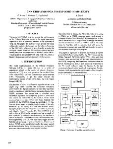
Marginal Unit Generation

j∈MG

This work gives explicit formulation of MG versus Load, i.e., MGj = q ( D∑2 , D∑ ) , and ∂MG j ∂D∑ = l ( D∑ ) .

j

j∈MG

MG

min j

j

× DF j +

× MGj +

D∑( 0 )

Present Load

DΣ Load

Fig. 1. Illustration of the difference between the perturbation-based sensitivity and the actual MG versus load formulation.

∑C

j∈NG

∑ NG

j∈NG

∑GSF

j∈NG

≤ MG j ≤ MG

k− j

max j

j

j

(1)

× NG j

× DF j − ∑ Di × DFi + Ploss = 0

(2)

i∈N

× NGj − ∑GSFk −i × Di ≤ Fkmax, ∀k ∈ Bc (3) i∈N

, ∀j ∈ MG

(4)

where DFi = 1 −

Perturbation approach gives numeric value of the slope of MG versus Load at the present operation point.

× MG j +

∂Ploss ∂Pi

Equation (1)-(4) models the power balance equation, power transmission line constraints and the goal of seeking minimum total fuel cost. Note that the power loss is considered in the power balance equation. Although an improved model [2] that distributes losses at each line rather than at the reference buses

4 can be applied, this paper uses the above model as it aligns with commonly used DCOPF model. It should be noted that staircase bidding price, namely, piece-wise linear cost function, is assumed in the model since it is the common practice in power markets. C. Characteristics Equations When load varies from a given operation point, the set of marginal units will remain the same as long as no new constraints become binding, including generation output constraints and transmission line limits. Therefore, within a certain range of load variation at any given operation point, the set of marginal units will keep unchanged, and the binding constraints remain binding. This load variation window is named Load Variation Range of Interest (LVRI) in this paper. The following study will be focusing on the LVRI. At any specific loading scenario, the solution of DCOPF model (1)-(4) will determine the sets of MG and NG. And the sets will remain unchanged during the LVRI around the given scenario. By taking out all the binding constraints in (2)-(3), a set of equalities are obtained

∑ MG

j∈MG

∑ GSF

j∈MG

j

× DF j +

k− j

∑ NG

j∈NG

× MG j +

j

× DF j − ∑ Di × DFi + Ploss = 0

∑ GSF

j∈NG

(5)

introducing the load variation participation factor, the variation patterns of load at all buses are incorporated into a set of factors, and thus it will facilitate the analysis on the system as a whole. Specifically, it could also be defined to reflect load variation at any single bus. More usefully, it could be designated to present load changes at several or all buses. By doing so, load impact analysis could be done from the perspectives of an individual bus, an area/system. In the latter case, the mutual interaction of load variation at different buses is considered. Various load variation participation factor could be employed for specific purposes. For instance, it could be defined as Di to model the load that changes at each bus D∑

proportionally to its base load. It could also be defined as 1 at one bus and all zeros at other buses in the case of LMP study. More complicated load variation pattern could be modeled by assigning piece-wise constants to the factors. Apply derivative to equations (5)-(6) w.r.t. D∑ , ∂MG j

∑ ( ∂D

j∈MG

i∈N

k− j

× NG j

∑ GSF

k− j

×

i∈N

and (6) equals to the number of variables ( MG j , j ∈ MG ), and normally only one solution exists. In other words, the number of marginal units should be equal to the number of congested lines plus 1, i.e., NMG=NBc+1 [1, 11]. For the DCOPF during a specific LVRI, on the other hand, the optimal solution is effectively determined by only the binding constraints because the feasible region constrained by all the binding constraints shrinks down to a single point. Therefore, equations (5)-(6) are essentially equivalent to DCOPF model (1)-(4) during the LVRI. It should be noted that the marginal unit generation pattern within a LVRI is not affected by the cost function because staircase constant bidding price is assumed. D. Marginal Unit Generation Sensitivity In order to make the generation sensitivity having the ability to predict future generator output, we need to apply a pre-defined load variation pattern into the system. Thus, load variation participation factor f i is introduced to represent the load variation pattern, fi =

ΔDi ΔD∑

(7)

The load variation participation factor is defined as the ratio of load change at each bus to the total load change. By

∂D∑

NG j ×

∂DF j

(8)

− ∑ GSFk −i × f i = 0, ∀k ∈ Bc

(9)

i∈N

∂MG j

∑

)+

∂D∑

∑

i∈N

j∈MG

It should be pointed out that the number of equations in (5)

∂DF j ∂D∑

− (∑ f i × DFi + ∑ Di ×

(6)

− ∑ GSFk −i × Di = Fkmax , ∀k ∈ Bc

× DF j + MG j ×

j∈NG

∂DFi ∂P ) + loss = 0 ∂D∑ ∂D∑

i∈N

It could be rewritten as

∑

j∈MG

DF j ×

∂MG j ∂D∑

=−

∑

j∈MG

MG j ×

∂DF j ∂D∑

−

+ ∑ f i × DFi + ∑ Di × i∈N

∑ GSF

j∈MG

k− j

×

∂MG j ∂D∑

i∈N

∑

j∈NG

NG j ×

∂DF j ∂D∑

(10)

∂DFi ∂Ploss − ∂D∑ ∂D∑

= ∑ GSFk −i × f i , ∀k ∈ Bc

(11)

i∈N

For simplicity, the right hand side of the equations are denoted by a and bk respectively. Then, equation (10)-(11) could be presented in matrix form as

⎡DF T ⎤ ∂MG ⎡a ⎤ (12) =⎢ ⎥ ⎢ ⎥ ⎣b ⎦ ⎣GSFMG ⎦ ∂D∑ Where GSFMG denotes the Generation Shift Factor of marginal unit with respect to congested transmission lines. Note that DF is a N MG × 1 vector; GSFMG is a ( N MG − 1) × N MG matrix; ∂MG is a N MG × 1 vector; a is a real ∂D∑ number (scalar); and b is a ( N MG − 1) × 1 vector.

It should be noted that quite a few parts of a are implicit functions of marginal unit generation (or total load), such as ∂DF j , ∂Ploss , therefore generally it is hard to solve (12) DFj , ∂D∑ ∂D∑ analytically.

5 IV. MUGS FORMULATIONS FOR SPECIAL CASES Equation (12) shows that MUGS is an implicit function of marginal unit generation, which is unknown variable itself. Fortunately, in some special scenarios, explicit formulation of MUGS can be derived, which is only a function of total load.

A. One Marginal Unit at the Reference Bus When there is a marginal unit at the reference bus, equation (12) could be solved symbolically. Suppose the bus numbers are reorganized so that the reference bus is the first bus. For reference bus, we have

DFi

i = ref bus

GSFk −i

=1

i = ref bus

(13)

= 0, ∀k ∈ B

(14)

B. Lossless Network For lossless network, equation (12) will be simplified as

⎤ ∂MG ⎡1 ⎤ ⎡1T =⎢ ⎥ ⎥ ⎢ ⎣b ⎦ ⎣GSFMG ⎦ ∂D∑

(19)

The solution of (19) is

So, equation (12) is rewritten as ⎡1 DF T ⎤ ∂MG ⎡a ⎤ =⎢ ⎥ ⎢ ⎥ ⎢⎣0 GSF MG ⎥⎦ ∂D∑ ⎣b ⎦

taking derivative of the original equations (5)-(6), which appears similar to the methods in [3-4], the explicit formulation (17) and (18) hold true within the LVRI, not just at the given operating point. Moreover, the formulations do not contain any unknown variable except load, therefore the generation at any load condition within the LVRI could be precisely predicted by using (17) and (18) for any pre-defined load variation pattern.

−1

(15)

⎤ ⎡1 ⎤ ∂MG ⎡1T =⎢ ⎥ ⎢ ⎥ ∂D∑ ⎣GSFMG ⎦ ⎣b ⎦

(20)

where DF and GSF MG are obtained by simply removing the reference bus associated column from DF and GSFMG ,

It means that the generation output sensitivities of all marginal units are constants in a no-loss system, which is reasonable.

respectively. Thus DF is a ( N MG − 1) × 1 vector, and GSF MG

C. Notes on Generation Output Sensitivity Calculation

is a ( N MG − 1) × ( N MG − 1) and invertible matrix. The analytical solution of equation (15) could be obtained as follows

When there is no power loss, the system is purely a linear system and therefore the marginal unit outputs are linear functions in terms of load. When loss is considered, the incurred incremental loss will be compensated by marginal units. If there is a marginal unit at the reference bus, all the loss will be picked up by this unit, and therefore the output of this marginal unit will follow a quadratic pattern while all the other marginal units keep the same linear pattern as in the lossless network. In fact, all marginal units except the one at the reference bus have the same value of sensitivities as those obtained from the corresponding lossless network. If there is no marginal unit at the reference bus, the incremental power loss will be split among all marginal units.

T −1 ∂MG ⎡ a − DF × GSF MG × b ⎤ ⎢ ⎥ = 1 ∂D∑ ⎢GSF −MG ⎥ b × ⎣ ⎦

(16)

It can be seen that the generation sensitivities of all marginal units except the one at the reference bus are constants. The values are only determined by GSF and load variation participation factor f. Therefore the generation outputs of these marginal units are linear function of total load MG j

j∈{MG \ ref bus}

= c1, j × D∑ + c 0 , j

(17)

V. TWO APPLICATIONS

where −1

c1 = GSF MG * b . Substituting (17) back into (16) could give the formulation of the generation sensitivity of the marginal unit at the reference bus as follows ∂MG j ∂D∑

= c11 × D∑ + c12

(18)

j = ref bus

where c11 ,c12 are constants (See Appendix A for detailed formulations for these two constants). It obviously shows that the generation output sensitivity at the reference bus is, instead of a constant, a linear function of total load. It is consistent with the expectation since all the power loss is picked up by the unit at the reference bus. It should be pointed out that, although it is derived by

In this section, basic ideas of applying the generation sensitivity in operation and planning are introduced to demonstrate the usefulness of generation sensitivity.

A. Congestion Prediction Most of the time, there are bottlenecks existing in contemporary power systems since historically the transmission systems were designed for local power transfer demands, instead of ensuring “Open Access” in today’s restructured environment [10]. Congestion management is therefore always a big issue in operation and planning, especially in the circumstances with emerging demands of transporting renewable and/or distributed energy. Generation Shift Factor (GSF) (also known as Power Transfer Distribution Factor) is frequently used for operation and planning purpose. GSF reflects the power flow change

6 pattern with generation variation; however, it does not address how the generation responses, under the cost-driven economic dispatch, to system variations like load changes. Moreover, GSF does not take into account the network constraints and generation limits when load changes. On the other hand, it is very helpful for the dispatchers to know how the power flow will change with respect to assumed load change pattern under the economic dispatch/OPF framework. Hence, Optimal Load Shifting Factor (OLSF), or, Optimal Load Transfer Distribution Factor (OLTDF), is proposed to provide this information. By “Optimal”, it means that the factors are subject to the optimal dispatch principle. In other words, OLSF follows both physical law and economic rules, and satisfies all physical limits as well, while GSF only obeys power balance law. OLSF is defined as,

OLSFk =

∂Fk , ∀k ∈ B ∂DΣ

(21)

It shows how much power flow in line k will change with respect to a specific load change pattern, which is implied in DΣ . Equation (21) can be rewritten as,

OLSFk =

∂Fk ∂F ∂P =∑ k × i ∂DΣ i∈N ∂Pi ∂DΣ

(22)

(∀i ∈ N)

= Gi − ( f i × DΣ + Di

( 0)

− f i × D∑ )

∂Pi ∂Gi = − fi ∂DΣ ∂DΣ

(23)

Substituting (23) into (22) gives ∂F ∂G ∂F OLSFk = k = ∑ k ( i − f i ) ∂DΣ i∈N ∂Pi ∂DΣ

=

∂F ∂Fk ∂MG j × − ∑ k × fi ∂DΣ i∈N ∂Pi j∈MG ∂Pj

=

∑ GSF

∑

j∈MG

k

k− j

×

∂MG j ∂DΣ

(24)

− ∑ GSFk −i × f i

k

ΔDΣ k could be obtained by simply establishing and solving

the following quadratic equations respectively. ) = MG max , ∀j ∈ MG j

(26)

f j ( DΣ( 0 ) + ΔDΣ j ) = MG min j , ∀j ∈ MG

(27)

f j ( D Σ( 0 ) + ΔD Σ

ub j

lb

f k ( DΣ( 0 ) + ΔDΣ

ub k

(28)

) = Fkmax , ∀k ∈ {B \ Bc}

lb

(29)

f k ( DΣ( 0) + ΔDΣ k ) = − Fkmax , ∀k ∈{B \ Bc}

Where fj is the function of marginal unit generation output for generator j; fk is the function of the line flow for branch k. Furthermore, the margin of load variation from present loading level to the one with a new binding constraint in load growth and load drop conditions are defined respectively as min

{ΔDΣ

ub

max

{ΔDΣ

ub

j∈MG, k∈B, ΔDΣ ≥ 0 j∈MG, k∈B, ΔDΣ < 0

j

j

, ΔDΣ j , ΔDΣ

lb

ub

lb

ub

, ΔDΣ j , ΔDΣ

k

k

lb

(30)

lb

(31)

, ΔDΣ k } , ΔDΣ k }

In fact, the margin of load variation is basically defined as the shortest one among all the load variation distances with the same sign. Once the margin is determined, the new binding constraint is identified simultaneously; no matter it is a generation or transmission constraint. Specifically, when generation sensitivities are constants, or, when linear approximation of generation is employed for studies where speed outweighs accuracy, OLSF are constants. Thus both generation and power flow follow purely linear pattern with respect to assumed load variation. In this case, load variation distances ΔDΣ ub , ΔDΣ lb , ΔDΣ ub and ΔDΣ lb j

j

i∈N

j

j

lb

k

k

could be calculated by

Especially, for each congested line,

OLSFk = 0, ∀k ∈ Bc

k

could vary until transmission line k is hitting its thermal limit in the downstream (upstream) direction for the first time. Then, load variation distances ΔDΣ ub , ΔDΣ lb , ΔDΣ ub and

ΔDΣm−arg in =

(0)

j

j

could vary from the given operating point until the upper (lower) limit of marginal generator j is reached for the first time. Similarly, let ΔDΣ ub ( ΔDΣ lb ) denotes how much load

ΔDΣm+arg in =

It is also known that

Pi = Gi − Di

demonstrates an explicit formulation and is a function of just the total system load, not coupled with any other unknown variable. Let ΔDΣ ub ( ΔDΣ lb ) denotes how much the system load

(25)

It is apparently another representation of the fact that every congested line will remain the current flow at the maximum limit, within interested load variation range. With generation sensitivity and OLSF, it is possible to predict the next binding constraint, such as new non-marginal unit or new congestion. It could be easily done when the generation sensitivity demonstrates a mathematically manageable pattern, such as linear, quadratic, etc. Fortunately, the generation sensitivity obtained by the proposed approach

ΔDΣ

ub

ΔDΣ

lb

ΔDΣ

=

j

j

ub k

=

=

− MG (j 0 ) MG max MG max − MG (j 0) j j = , ∀j ∈ MG (32) ∂MG j c1, j ∂DΣ MG (j 0 ) − MG min MG min − MG (j 0) j j = , ∀j ∈ MG ∂MG j c1, j ∂DΣ

Fkmax − Fk( 0) = OLSFk

Fkmax − Fk( 0 )

∑ GSF

j∈MG

k− j

× c1, j − ∑ GSFk −i × f i i∈N

, ∀k ∈ B

(33)

(34)

7 ΔDΣ

lb k

=

− Fkmax − Fk( 0 ) = OLSFk

− Fkmax − Fk( 0)

∑ GSF

j∈MG

k− j

×c1, j − ∑ GSFk −i × f i

, ∀k ∈ B

(35)

i∈N

The idea of quickly identifying the next binding generation limit or transmission limit is shown in Figure 2 and Figure 3. For simplicity, the generation sensitivity and OLSF are drawn as perfectly linear curves in these two figures. The slopes of these lines are amplified for illustration purpose. Note that in Figure 3, power flow through line k+3 is always kept at its maximum capacity and has OLSFk+3 as zero. Only the load variation distances for marginal generator j and transmission line k are drawn in these two figures for better illustration.

to calculate the LMP, which serves a purpose for settlement and as the ‘invisible hand’ to guide market participants activities. Various approaches have been proposed to calculate LMP, the components of LMP, and LMP sensitivity [5, 7-8]. Marginal unit output sensitivity offers a chance for calculating and predicting LMP and its sensitivity. According to the definition, Locational Marginal Price could be written as ∂MG j (36) LMPi = ∑ C j × ∂Di j∈MG Where ∂MG j can be easily obtained by setting load variation ∂Di

participation factor to be 1 at bus i and zeros at all other buses. ∂MG j ∂MG j (37) = ∂Di

∂DΣ

f j = 0, j ≠ i f i =1

VI. CONCLUSIONS

Fig. 2. Demonstration of Using Generation Sensitivity to Locate Possible Binding of Generation Constraints.

Fig. 3. Demonstration of Using OLSF to Locate Possible Binding of Transmission Constraints.

It should be pointed out that once the actual load variation exceeds ΔDΣ+ or ΔDΣ− , a new constraint will be binding, in the case of both load growth and load decrease. With the presence of the new binding constraint, the set of marginal units and non-marginal units will change, and hence the system will be operating at a new operating point with a new set of marginal units and binding constraints. Correspondingly, Figure 2 and Figure 3 will be redrawn around the new operating point. Moreover, accompanied by the appearance of a new binding constraint, there will be a simultaneous disappearance of an existing binding constraint. m arg in

m arg in

B. LMP Calculation In power market operation, the primary and crucial task is

This paper firstly introduces the concept of load variation range of interest (LVRI), within which existent binding constraints remain binding, and no new constraints come into play. In this range, the DCOPF could be essentially represented by the binding constraints. In addition, load variation participation factor is introduced to help define various load change pattern. Second, explicit formulations for MUGS are derived for some special cases, which show MUGS is strictly a linear function or constant with respect to total system load. The function has only one independent variable, system load, and therefore it offers the convenience to predict future generation directly. Third, two potential applications of the generation sensitivity are discussed. One application is congestion prediction. Regarding the limitation of GSF, firstly OLSF is proposed to reflect the power flow change with assumed load variation under OPF framework. Then the methodology is demonstrated by employing OLSF and generation sensitivity information to identify the amount of load variation that causes any specific unbinding constraint to be binding. Hence, the margin from present operating point to another point with a new binding constraint can be easily calculated. This information is very useful for dispatchers in operation and planning. Generation sensitivity is also demonstrated to calculate LMP and its sensitivity as another application. With the generation sensitivity as a function of load, LMP sensitivity can be easily calculated not only at the present loading level, but any other loading level within LVRI. Naturally, generation sensitivity is also helpful for GENCO to predict generation dispatch at future load scenarios. VII. REFERENCES [1] [2]

Fangxing Li, “Continuous Locational Marginal Pricing (CLMP),” IEEE Trans. on Power Systems, vol. 22, no. 4, pp. 1638-1646, November 2007. Fangxing Li and Rui Bo, “DCOPF-Based LMP Simulation: Algorithm, Comparison with ACOPF, and Sensitivity,” IEEE Trans. on Power Systems, vol. 22, no. 4, pp. 1475-1485, November 2007.

8 [3]

A. J. Conejo, E. Castillo, R. Minguez, and F. Milano, “Locational Marginal Price Sensitivities,” IEEE Trans. on Power Systems, vol. 20, no. 4, pp. 2026-2033, November 2005. [4] Xu Cheng and T. J. Overbye, “An energy reference bus independent LMP decomposition algorithm,” IEEE Trans. on Power Systems, vol. 21, no. 3, pp. 1041-1049, Aug. 2006. [5] E. Litvinov, T. Zheng, G. Rosenwald, and P. Shamsollahi, “Marginal Loss Modeling in LMP Calculation,” IEEE Trans. on Power Systems, vol. 19, no. 2, pp. 880-888, May 2004. [6] Rui Bo, Fangxing Li and Chaoming Wang, "Congestion Prediction for ACOPF Framework Using Quadratic Interpolation," Proceedings of the IEEE Power Engineering Society General Meeting 2008, Pittsburgh, USA, 2008. [7] T. Orfanogianni and G. Gross, “A General Formulation for LMP,” IEEE Trans. on Power Systems, vol. 22, no. 3, pp. 1163-1173, Aug. 2007. [8] Kai Xie, Yong-Hua Song, John Stonham, Erkeng Yu, and Guangyi Liu, “Decomposition Model and Interior Point Methods for Optimal Spot Pricing of Electricity in Deregulation Environments,” IEEE Trans. on Power Systems, vol. 15, no. 1, pp. 39-50, Feb. 2000. [9] Fangxing Li, Jiuping Pan and Henry Chao, “Marginal Loss Calculation in Competitive Spot Market,” Proceedings of the 2004 IEEE International Conference on Deregulation, Restructuring and Power Technologies (DRPT), vol. 1, pp. 205-209, April 2004. [10] D. J. Morrow and Richard E. Brown, “Future vision - The Challenge of Effective Transmission Planning,” IEEE Power and Energy Magazine, vol. 5., no. 5, pp. 36-45, 2007. [11] D. Kirschen and G. Strbac, Fundamentals of Power System Economics, John Wiley and Sons, 2004.

D i = Di

( 0)

+ ΔDi = Di

= f i × D ∑ + Di

(0)

( 0)

+ f i × ΔD ∑ = Di

− f i × D∑

Fk =

∑ GSF

k− j

j∈MG

∑ GSF

=

j∈{MG \ ref bus }

k− j

× MG j +

i∈N

(A.1)

= ∑ GSFk −i (Gi − Di )

∑ GSF

j∈NG

k− j

k− j

( 0)

(A.3)

(0)

− fi × D∑ )

∑ GSF

i∈N

× NG j (0)

− fi × D∑ )

Substituting (17) into (A.3) gives Fk =

∑ GSF

j∈{MG \ ref bus }

k− j

(c1, j × D∑ + c0, j ) +

− ∑ GSFk − i ( f i × D∑ + Di

( 0)

∑ GSF

=(

k− j

j∈{MG \ ref bus }

k− j

× NG j

(0)

(A.4)

× c1, j − ∑ GSFk − i × fi ) DΣ i∈N

∑ GSF

+

∑ GSF

j∈NG

− f i × D∑ )

i∈N

k− j

×c0, j +

( 0)

i∈N

∑ GSF

j∈NG

k− j

× NG j

(0)

− fi × D∑ )

Δ

= c3, k × DΣ + c4, k

Delivery factor is formulated as DFi = 1 −

(

∂PLoss ∂ 2 =1− ∑ Fk × Rk ∂Pi k∈B ∂Pi

)

= 1 − ∑ 2 × Fk × GSFk −i × Rk k∈B

(A.5)

= 1 − ∑ 2 × Rk × GSFk −i (c3,k × DΣ + c 4,k ) k∈B

= (− ∑ 2 × Rk × GSFk −i × c3,k ) × DΣ k∈B

− ∑ 2 × Rk × GSFk −i × c 4,k + 1 k∈B

Δ

= c5,i × DΣ + c6,i

=

× NG j − ∑ GSFk −i × Di i∈N

⎛

∑ ⎜⎜ 2 × F

k∈B

=

i∈N

× MG j +

× NG j

( 0)

j∈NG

− ∑ GSFk −i ( fi × D∑ + Di

(

Fk = ∑ GSFk −i × Pi

k− j

k− j

i∈N

∂PLoss ∂ 2 Fk × Rk =∑ ∂ D ∂DΣ k∈B Σ

Power flow through line k is written as

∑ GSF

j∈NG

First order derivative of power loss w.r.t. total load is written as

A. Derivation of equation (18)

j∈MG

∑ GSF

× MG j +

− ∑ GSFk − i ( Di

IX. APPENDIX

=

(A.2)

(0)

− ∑ GSFk −i ( fi × D∑ + Di

VIII. BIOGRAPHIES

Fangxing (Fran) Li (S’98, M’01, SM’05) received his BSEE and MSEE degrees both from Southeast University (China) in 1994 and 1997, respectively, and then his Ph.D. degree from Virginia Tech in 2001. He has been an Assistant Professor at The University of Tennessee (UT), Knoxville, TN, USA, since August 2005. Prior to joining UT, he worked at ABB, Raleigh, NC, as a senior engineer and then a principal engineer for four and a half years. At ABB, he was the lead developer of GridViewTM, ABB’s market simulation tool. His current research interests include power market, reactive power, renewable and distributed generation, distribution systems, and reliability. He is a registered Professional Engineer (P.E.) in the state of North Carolina.

(0)

+ f i ( D∑ − D∑ )

For the case with a marginal unit at the reference bus, equations (13)-(14) hold true. Therefore, (A.1) is rewritten as

j∈{MG \ ref bus }

Rui Bo (S’02, M’09) received the B.S. and M.S. degrees in electric power engineering from Southeast University (China) in 2000 and 2003, respectively, and then his Ph.D. degree from University of Tennessee, Knoxville, TN in 2009. He worked at ZTE Corporation and Shenzhen Cermate Inc. from 2003 to 2005, respectively. He is presently working at an Indpendent System Operator in the US. He won the 2nd Place Prize Award at the Student Poster Contest at the IEEE PES 2009 Power Systems Conference and Exposition (PSCE), held in March 2009, Seattle, WA, USA.

(0)

⎝

∑ [ 2 × (c

k∈B

k

×

⎞ ∂Fk × Rk ⎟⎟ ∂DΣ ⎠

(A.6)

× DΣ + c 4 , k ) × c 3 , k × R k ]

3, k

= [ ∑ ( 2 × c 3 , k × R k ) ] × DΣ + ∑ ( 2 × c 3 , k × c 4 , k × R k ) 2

k∈B

By definition of load variation participation factor in (7), we have

)

k∈B

Δ

= c 7 × DΣ + c 8

Finally, scalar a defined in (12) is derived as follows,

9 Δ

∑

a =−

j∈MG

MG j ×

∂DF j ∂D∑

i∈N

∑

j∈{ MG \ ref bus }

MG j ×

i∈N

∑ (c

NG j ×

∂DF j ∂D∑

∑

−

∂D∑

NG j ×

j∈NG

+ ∑ f i × DFi i∈N

∂DF j ∂D∑

∑ NG

× D∑ + c 0 , j ) × c5, j −

1, j j∈{ MG \ ref bus }

∂DF j

+ ∑ f i × DFi i∈N

∂DFi ∂Ploss − ∂D∑ ∂D∑

+ ∑ Di × =−

∑

j∈NG

∂DFi ∂Ploss − ∂D∑ ∂D∑

+ ∑ Di × =−

−

j∈NG

j

× c5, j

+ ∑ f i ( c 5 ,i × D Σ + c 6 ,i ) i∈N

+ ∑ ( f i × D ∑ + Di

(0)

i∈N

= (−

∑c

1, j j∈{MG \ ref bus }

−

× c 5 , j + 2 × ∑ f i × c 5 , i − c 7 ) × DΣ i∈N

∑c

0, j j∈{ MG \ ref bus }

+ ∑ ( Di

(0)

− f i × D ∑ ) × c 5 , i − (c 7 × DΣ + c 8 )

( 0)

i∈N

× c5, j −

∑ NG

j

j∈NG

× c 5 , j + ∑ f i × c 6 ,i i∈N

(0)

− f i × D∑ ) − c8

Δ

= c 9 × D∑ + c10

(A.7) Δ

−1 If we define GSFMG * b = α = [α 1 α 2 ⋅ ⋅ ⋅ α N MG −1 ]T , then the

generation sensitivity of marginal unit at the reference bus is derived as ∂MG j ∂D∑

−1 = a − DF T × GSFMG ×b j = ref bus

= c9 × D∑ + c10 − = (c9 − −

∑ (c

× DΣ + c 6 , j ) × α j

∑c

× α j ) × DΣ + c10

∑c

×α j

5, j j∈{MG \ ref bus }

5, j j∈{MG \ ref bus }

6, j j∈{MG \ ref bus }

Δ

= c11 × D∑ + c12

Thus, equation (18) is obtained.

(A.8)