Macroeconomic E¤ects of the Demographic Transition in Brazil Ricardo D. Brito
Carlos Carvalho
Insper
PUC-Rio August 2014
Abstract Brazil is a developing country with a relatively young population that is undergoing a fast demographic transition. The dependency ratio – the economically inactive population to the labor force – should hit bottom in ten years, and start increasing fast thereafter. Hence, the so-called “…rst demographic dividend” –an increase in the size of the labor force relative to the overall population – will soon turn negative and subtract from per capita growth. However, a “second demographic dividend” is possible if, facing the prospects of an extended period of retirement, individuals decide to increase the pace of asset accumulation. We use an overlapping generations model to study the possibility of a meaningful second dividend materializing in Brazil. Our conclusion is that this is an unlikely outcome. The main culprit is a generous social security system that considerably undermines households’incentives to save for retirement. JEL classi…cation codes: E13, E60, J11 Keywords: demographic transition, Brazil, capital ‡ows, social security, demographic dividend
This paper was commissioned by the CEDES-IDRC project “Demographic asymmetries and global …nancial governance.” We thank Ramiro Albrieu, Pablo Comelatto, Jose Fanelli, Martin Rapetti, Marcelo Santos, Cassio Turra, and seminar participants at EBE 2013, CEDES/UBA and Insper for valuable comments and discussions. Felipe Alves and Felipe Mazin provided research assistance. Emails:
[email protected],
[email protected].
1
1
Introduction
Brazil is a relatively young, prominent developing country undergoing what is expected to be a fast demographic transition. Owing to a decline in the mortality rate, the Brazilian population increased signi…cantly between 1940 and 1970. In the 1940s, the annual population growth rate was around 2:4%, rising to 3:0% in the 1950-1960s, as life expectancy rose from 44 to 54 years. According to Carvalho (2004), the so-called “demographic transition” in Brazil started in the 1970s, with a sudden fall in the fertility rate. The latter kept decreasing since then, leading to important di¤erences between the actual age distribution of the population and its so-called “stable-equivalent.”1 At the same time, longevity kept increasing. By 2010, population growth had fallen to only 1:0% per year, life expectancy had reached 74 years, and the economically active population had grown from 56% to 64% of the total population (between 1980 and 2010). According to recent forecasts, population growth is expected to fall further, entering negative territory around 2050. A useful summary of the population’s age structure, the total dependency ratio –the size of the population that is economically inactive to the size of the labor force – has been falling continuously since the peak attained around 1965. That ratio is now expected to hit bottom within the next ten years, before increasing again to reach a level close to its historical peak by the end of this century.2 It is well known that demographic developments may have important macroeconomic consequences. In particular, increases in longevity and decreases in population growth – which are features of modern demographic transitions such as the one Brazil is undergoing – have important implications for savings decisions, capital accumulation, and, ultimately, economic growth and well-being. Such “aging processes”may also present important challenges for public …nances, depending on social security arrangements. In turn, because such arrangements are important determinants of consumption-savings decisions, they also shape the way in which demographic developments in‡uence the macroeconomy.3 In this chapter, we study the macroeconomic e¤ects of the demographic transition in Brazil. A common way to analyze the potential e¤ects of demographic developments on the economy is to focus on the possibility of so-called “demographic dividends” arising during a demographic transition. The …rst demographic dividend starts after a fall in fertility leads the labor force to grow relatively faster than the overall population, thus spurring per-capita income. At a later stage, lower fertility leads to lower labor force growth, while increases in longevity drive higher the population share of the elderly. As a result, the dependency ratio increases again 1
The stable-equivalent population is the underlying population that would emerge if the fertility and mortality rates remained constant for a long period of time. 2 United Nation’s World Population Prospects: The 2012 Revision. The total dependency ratio is computed as the ratio of the sum of the population aged 0-14 and that aged 65+ to the population aged 15-64. 3 It is also well known that economic developments may a¤ect demographic trends (see, e.g., Galor 2011). In this paper we take demographic developments to be exogenous, and study their macroeconomic consequences.
2
and reverses the …rst dividend. Brazil is close to the end of its …rst demographic dividend: The labor force should soon start growing less than the overall population. We thus focus on the possibility of a second demographic dividend arising during the remainder of Brazil’s demographic transition. The second demographic dividend may arise if, facing the prospects of an extended period of retirement, individuals decide to increase the pace of asset accumulation (Mason and Lee 2007). This leads to either larger domestic capital stock or larger foreign asset holdings. In either case, domestic income ends up being higher. Whether or not a second dividend materializes during the aging process depends crucially on the extent to which individuals need to save for retirement, which in turn depends on social security and other institutional and cultural arrangements. At …rst pass, the current social security system does not bode well for the prospects of a meaningful second demographic dividend in Brazil. According to Turra, Queiroz, and Rios-Neto (2011), the Brazilian social security system is particularly generous toward the elderly. Because Brazil is a developing country with a (still) young population, one could expect public transfers to be directed to children. Instead, as in older, developed Western countries, social programs to the elderly dominate public transfers, while children’s well-being depends largely on individual household e¤orts. This arrangement certainly a¤ects households’incentives to save for retirement. However, in an open economy, lack of domestic savings need not hold back the pace of capital accumulation, which can be …nanced with foreign savings. All else equal, the existence of di¤erences in the intensity, pace, and timing of demographic transitions across countries should in‡uence the direction and size of international capital ‡ows. Whether or not capital will ‡ow to Brazil during the remainder of its demographic transition thus depends, among many other things, on its demographic developments relative to those elsewhere in the global economy. To study how public policies and di¤erential demographic developments vis-a-vis the world might interact to produce or prevent a second demographic dividend in Brazil, we use a smallscale, two-country, general-equilibrium overlapping generations model (OLG), based on Gertler (1999) and Ferrero (2010) – with the “foreign country” representing the rest of the (more developed) world. We keep the open economy dimension of Ferrero (2010) and reintroduce social security systems, as in Gertler (1999). The framework allows us to model di¤erential demographic trends, social security systems, …scal policies, retirement ages etc., and to study the role of demographics and policies in shaping a second demographic dividend in Brazil. To isolate the role of demographic developments in Brazil and abroad from other factors that can impact the variables of interest, those developments are the only forces driving the economies from one steady state to another. We also study the importance of international capital ‡ows, by contrasting results for open- and closed-economy versions of the model. Our results suggest that, given the current social security system, a small second demo-
3
graphic dividend would arise in Brazil if it remained relatively closed to trade in goods and assets. Opening up under current social security arrangements turns out to be a losing proposition in that respect. However, scenarios in which current social security arrangements are maintained produce incredible paths for some variables, such as expenditures with public pensions and taxes as a share of Gross Domestic Product (GDP). This is due to the fact that maintaining the very high replacement rates currently in place in Brazil becomes unsustainable as the country starts to age fast in the next couple of decades. Motivated by those results we then entertain “reform scenarios,”in which growth in expenditures with public pensions is contained. We …rst analyze a “bold” reform scenario in which expenditures with public pensions are frozen as a share of GDP, and the replacement rate has to adjust endogenously to balance the budget. This produces a more meaningful second demographic dividend in Brazil, irrespective of whether the economy is open or closed to trade. In fact, in that case becoming more integrated with the world economy arguably becomes a winning proposition. However, the bold reform scenario is arguably unrealistic, since it involves defaulting on “contracts” that are currently in place. Hence we consider a more gradual reform scenario, in which the replacement rate in Brazil is lowered to the level that prevails in the OECD over a 25 year period. That brings us back to a situation in which a closed economy might arguably deliver a larger second dividend. We conclude that a meaningful second dividend is unlikely to materialize in Brazil. The main culprit is a generous social security system that considerably undermines households’ incentives to save for retirement. We grant that there exist reforms that would be able to spur a meaningful second dividend, but our results indicate that they would need to be too aggressive to appear feasible. Our work is related to two intersecting literatures. The …rst uses large-scale overlapping generations models to study social security systems, evaluate policy reforms, and perform counterfactual analyses. Examples include Imrohoroglu et al. (1995), Attanasio et al. (2006, 2007), and Krueger and Ludwig (2007). In work applied to Brazil, Barreto (1997), Barreto and Oliveira (2001), and Ellery Jr. and Bugarin (2003) compare the pay-as-you-go social security scheme with a fully savings-funded system. The second literature studies the macroeconomic e¤ects of demographic developments. Examples include Ferrero (2010), Mason and Lee (2007) and Albrieu and Fanelli (2013). Like the last two papers, we focus on the second demographic dividend. Relative to those two papers, our work di¤ers in that we rely on a framework in which the consumption-savings decisions that are key to the second demographic dividend are endogenous. In other words, we emphasize what demographers call the behavioral dimension of the second dividend. We present a quantitative analysis of the e¤ects of the demographic transition on households’consumption-saving
4
decisions, and its implications for asset accumulation, current account dynamics, and capital ‡ows. Our work is closest to Attanasio et al. (2006, 2007). They use a large-scale, two-country, general-equilibrium OLG model to study the e¤ects of demographic developments on the macroeconomy, with a focus on social security. Both papers take a “North-South” perspective, and calibrate the model to data for the “More Developed Regions” and “Less Developed Regions” de…ned according to the UN’s classi…cation.4 In particular, Attanasio et al. (2006) take the point of view of developing economies to study the macroeconomic implications of di¤erential demographic transitions and social security systems in the North and in the South. However, Brazil does not …t their typical developing economy, which features relatively more favorable demographic trends going forward and much lower replacement rates than in the North.
The analytical framework5
2
As in Gertler (1999) and Ferrero (2010), the economic actors in the model are households, …rms, and the government. Individuals are born workers and supply inelastically one unit of labor while in the labor force.6 Income is either consumed or saved using the available assets: physical capital, government bonds, and foreign assets (in the open-economy versions of the model). Retirees consume out of their wealth and social security bene…ts. Goods producing …rms are perfectly competitive and produce the homogeneous consumption good. The government consists of a …scal authority that, takes government consumption and social security spending as given and relies on lump-sum taxes and one-period debt to satisfy its budget constraint. In our quantitative analyses we also consider cases in which expenditures with public pensions as a share of GDP are exogenously …xed and the replacement rate adjusts endogenously to balance the budget. We consider the e¤ects of changes in demographic parameters in an otherwise perfectforesight environment. The only source of uncertainty that may potentially a¤ect agents’behavior stems from idiosyncratic retirement and death risk. This approach isolates the e¤ects of demographics on the macroeconomic equilibrium, and is thus suitable for our goals. For brevity, below we present the structure of the domestic economy. The foreign economy is analogous. 4
According to the UN’s classi…cation, the group of “More Developed Regions”is composed of North America, Europe, Japan, Australia, and New Zealand. The group of “Less Developed Regions” includes Africa, Asia (except for Japan), Latin America and the Caribbeans, plus Melanesia, Micronesia, and Polynesia. 5 We follow Gertler’s (1999) and Ferrero’s (2010) presentation closely, maintaining a social security system as in Gertler (1999) and analysing open economies as in Ferrero (2010). We then use the model to de…ne demographic objects of interest – in particular the …rst and second demographic dividends, following Albrieu and Fanelli (2013), and Mason and Lee (2007). 6 Our model thus abstracts from childhood, as in Gertler (1999) and Ferrero (2010). We return to this issue when we detail the calibration on which we base our quantitative analysis.
5
2.1
Households and life-cycle structure
At any given point in time, individuals belong to one of two groups: workers (w) or retirees (r). At time t 1, workers have mass Ntw 1 and retirees have mass Ntr 1 . Between periods t 1 and t, a worker remains in the labor force with probability ! t 1 , and retires otherwise. If retired, an individual survives from period t 1 to period t with probability t 1 . In period t, (1 ! t 1 + nt 1 ) Ntw 1 new workers are ready to work. This life-cycle structure implies the following law of motion for the aggregate labor force: Ntw = (1
!t
1
+ nt 1 ) Ntw 1 + ! t 1 Ntw 1 = (1 + nt 1 ) Ntw 1 :
According to (1), nt 1 corresponds to the growth rate of the labor force between periods t and t. The number of retirees evolves according to Ntr = (1
! t 1 ) Ntw 1 +
r t 1 Nt 1 :
(1) 1
(2)
From (1) and (2), we de…ne the (elderly) dependency ratio ( t Ntr =Ntw ), which summarizes the relevant demographic dimension of the model, and evolves according to (1 + nt 1 )
t
= (1
!t 1) +
t 1
t 1:
(3)
Workers supply one unit of labor inelastically, while retirees do not work. Preferences for an individual of group z = fw; rg are de…ned recursively, based on a non-expected utility family (Kreps and Porteus 1978, Epstein and Zin 1989), and imply risk neutrality: z t
Vtz = f(Ctz ) +
1
[Et (Vt+1 j z)] g ;
(4)
where Ctz denotes consumption and Vtz stands for the value of utility in period t. Retirees and workers have di¤erent discount factors to account for the probability of death z t
=
(
if z = r; if z = w:
t
The expected continuation value in (4) di¤ers across workers and retirees because of the di¤erent possibilities to transition between groups Et fVt+1 j zg =
(
r Vt+1 w ! t Vt+1 + (1
r ! t ) Vt+1
if z = r; if z = w:
The analytical tractability of this life-cycle model comes from the fact that the transition
6
probabilities ! and are independent of age and of the time since retirement. With standard risk-averse preferences, however, the associated “retirement lottery” generates too strong a precautionary savings motive for young agents. Risk-neutral preferences with respect to income ‡uctuations eliminate this problem (Farmer 1990, Gertler 1999). Freedom to calibrate the coe¢ cient of intertemporal substitution ( (1 ) 1 ) then allows us to obtain a reasonable response of consumption and savings to changes in interest rates. Households consume a homogeneous …nal good Ct and allocate their wealth in physical capital Kt , bonds issued by the government Bt , and foreign assets Ft . Households rent the capital stock to goods producers at a (world) real rate RW;t plus the cost of depreciation 2 (0; 1). Government bonds Bt also pay a gross nominal return RW;t . 2.1.1
Retirees
An individual born in period j and retired in period chooses consumption Ctr (j; ) and assets Art (j; ) Ktr (j; ) + Btr (j; ) + Ftr (j; ), for t to solve Vtr (j; ) = max
(Ctr (j; )) +
t
r Vt+1 (j; )
1
(5)
subject to Ctr (j; ) + Art (j; ) =
RW;t
1
Art 1 (j; ) + Dt (j; ) ;
(6)
t 1
where Dt (j; ) is the retiree social security bene…t. At the beginning of each period, retirees turn their wealth over to a representative mutual fund which invests the proceeds in available assets (Kt , Bt , Ft ) and pays back a fair premium over the market return equal to 1= t 1 to compensate for the probability of death (Blanchard 1985, Yaari 1965). Investment decisions are made at the end of each period. The consumption Euler equation for the retiree yields that consumption is a fraction t t of total wealth RW;t 1 Art 1 (j; ) r Ct (j; ) = t t + St (j; ) ; (7) t 1
where St (j; ) is the total present value of the retiree’s future social security bene…ts (Dt+v (j; )) St (j; ) =
1 X v=0
Dt+v (j; ) v Q
RW;t+s 1 =
= Dt (j; ) +
t+s 1
St+1 (j; ) ; RW;t = t
(8)
s=1
and the marginal propensity to consume satis…es a …rst-order non-linear di¤erence equation 1 t t
=1+
RW;t1
t
7
1 t+1 t+1
:
(9)
From (6) and (7), asset holdings evolve according to Art (j; ) +
t St+1 (j;
)
RW;t
= (1
t
t)
RW;t 1 Art 1 (j; )
+ St (j; ) :
t 1
Finally, we can also show that the value function for a retiree is linear in consumption Vtr (j; ) = ( 2.1.2
t t) 1
Ctr (j; ) :
(10)
Workers
Workers start their life with zero assets. We write the optimization problem for a representative Ktw (j) + Btw (j) + Ftw (j). Speci…cally, worker born in period j in terms of total assets Aw t (j) such worker chooses consumption Ctw (j) and assets Aw j to solve t (j) for t Vtw (j) = max
(Ctw (j)) +
w ! t Vt+1 (j) + (1
r ! t ) Vt+1 (j; t + 1)
1
(11)
subject to w w Ctw (j) + Aw t (j) = RW;t 1 At 1 (j) + Wt Nt (j)
Tt (j) ;
(12)
w and Aw j (j) = 0, where Wt is the real wage, Nt (j) is the measure of cohort j, and Tt (j) is the r (j; t + 1) is the total amount of taxes paid by workers in that cohort. The value function Vt+1 solution of the retiree problem (5) (6) above and enters the continuation value in the dynamic program, since workers have to take into account the possibility that retirement occurs between periods t and t + 1. The complete solution to a worker’s optimization problem is described in detail in Gertler (1999) and Ferrero (2010). Workers’consumption is a fraction of total wealth, de…ned as the sum of …nancial and non-…nancial (“human”) wealth
Ctw (j) =
t
w RW;t 1 Aw t 1 (j) + Ht (j) + St (j) ;
(13)
where Ht (j) denotes the present discounted value of current and future real wages net of taxation Ht (j)
1 w X Wt+v (j) Nt+v (j) Tt+v (j) = Wt (j) Ntw (j) v Q v=0 t+s RW;t+s 1 =! t+s 1
Tt (j) +
! t Ht+1 (j) ; t+1 RW;t
(14)
s=1
and Stw (j) is the total present value of the future social security bene…ts the worker can expect
8
during retirement Stw (j) = (1
1
!t)
t+1
S w (j) St+1 (j; t + 1) + ! t t+1 ; t+1 RW;t t+1 RW;t
(15)
where St+1 (j; t + 1) = St+1 and St+1 denotes the present value of future social security t+1 Nt+1 bene…ts of all retirees alive at time t + 1. As for retirees, workers’ marginal propensity to consume t also evolves according to a …rst-order non-linear di¤erence equation: 1
=1+
(
t+1 RW;t )
1
1
t
The adjustment term
t+1
:
(16)
t+1
that appears in (14)-(16) corresponds to ! t + (1
t+1
!t) (
t+1 )
1 1
;
and augments the discount rate RW;t relative to the in…nite-horizon case. In the de…nition of non-…nancial wealth (14), the term t+1 RW;t =! t constitutes the real e¤ective discount rate for a worker. The dynamics of asset holdings can then be obtained from the worker’s budget constraint and the consumption function (13) Aw t (j) +
w ! t Ht+1 (j) + St+1 (j) = (1 t+1 RW;t
t)
w RW;t 1 Aw t 1 (j) + Ht (j) + St (j) :
Finally, as for retirees, workers’value function is also linear in their consumption Vtw (j) = ( t ) 1 Ctw (j) : 2.1.3
(17)
Aggregation
The marginal propensities to consume of workers and retirees are independent of individual characteristics. Hence, given the linearity of the consumption functions, aggregate consumption of workers (Ctw ) and retirees (Ctr ) have the same form as (7) and (13) 7 Ctw =
t
w RW;t 1 Aw t 1 + Ht + St ;
(18)
P r P w P Note the algebra for the aggregate variables: Art 1 = At 1 (j; ), Aw At 1 (j), Tt = Tt (j) , t 1 = j; P j j P P P Dt (j; ) = Dt , Ht = Ht (j) , Stw = Stw (j) and St = St (j; ). And, provided Wt (j) is independent j; j j P j; of individual-speci…c characteristics (i.e. equal to Wt 8 j): Wt (j) = Ntw Wt . 7
j
9
Ctr =
RW;t 1 Art
t t
1
(19)
+ St ;
where Azt 1 is the total …nancial wealth that members of group z = fw; rg carry from period t 1 into period t; Ht is the aggregate value of human wealth, evolving according to Ht = Wt Ntw
Tt +
! t Ht+1 ; (1 + nt ) t+1 RW;t
(20)
St is the present value of future social security bene…ts of all retirees alive at time t St = Dt +
Sbt+1 Ntr St+1 t = Dt + ; RW;t = t (1 + nt ) t+1 RW;t = t
(21)
with Dt for the total social security payments for retirees in period t, Sbt+1 = NSt+1 = St+1 r w t+1 Nt+1 t+1 w for the value of social security at t + 1 per bene…ciary; and St is the present value of future social security bene…ts that all workers alive at time t can expect during retirement 1
Stw = (1
!t)
= (1
!t)
1
t+1 1 1
t+1
Sbw N w Sbt+1 Ntw + ! t t+1 t t+1 RW;t t+1 RW;t w St+1 St+1 + !t ; (1 + nt ) t+1 t+1 RW;t (1 + nt ) t+1 RW;t
(22) (23)
Sw
w = Nt+1 for the value of future social security that workers alive at t + 1 can expect with Sbt+1 w t+1 during retirement per bene…ciary. The aggregate consumption function Ct is the weighted sum of (19) and (18). If t Art =At denotes the share of total …nancial wealth At held by retirees, the aggregate consumption function is
Ct =
t
[(1
t 1 ) RW;t 1 At 1
+ Ht + Stw ] +
t t
(
t 1 RW;t 1 At 1
+ St ) :
(24)
The distribution of assets across cohorts is a state variable that keeps track of the heterogeneity in wealth accumulation due to the life-cycle structure. Aggregate assets for retirees depend on the total savings of those who are retired in period t as well as on the total savings of the fraction of workers who retire between periods t and t + 1 Art = RW;t 1 Art
1
+ Dt
Ctr + (1
w ! t ) RW;t 1 Aw t 1 + Wt Nt
Tt
Ctw :
(25)
Aggregate assets for workers depend only on the savings of the fraction of workers who remain in the labor force w w Tt Ctw : (26) Aw t = ! t RW;t 1 At 1 + Wt Nt 10
The law of motion for the distribution of …nancial wealth across groups obtains from substituting expressions (18) and (26) into (25) (
1 + !t)
t
At = (1 !t
t t ) RW;t 1 t 1 At 1
+ Dt
Expression (27) relates the evolution of the distribution of wealth position At .
2.2
(27)
t t St :
t
to the aggregate asset
Production
The economy is competitive and producers combine labor and capital rented from both workers and retirees to produce according to a standard Cobb-Douglas labor-augmenting technology Yt = (Xt Ntw ) Kt1
1
(28)
;
where 2 (0; 1) is the labor share and the technology factor Xt grows exogenously at rate xt between t 1 and t Xt = (1 + xt 1 )Xt 1 :
1
The …rms choose Ntw , It to solve V (It 1 ; Kt 1 ) = max (Xt Ntw ) Kt1 It ;Kt
Wt Ntw
1
It +
V (It ; Kt ) RW;t
(29)
subject to capital adjustment costs Kt = (1
) Kt
1
"
2
It
+ 1
2
It
t
1
#
(30)
It :
The …rst-order conditions for labor, capital and investment are Yt Wt = w = X t Nt qt RW;t = (1
)
Kt 1 Ntw
Yt+1 + (1 Kt
1
;
(31)
) qt+1 ;
(32)
and "
qt 1
2
It 2
It
1
t
It It
It 1
t
It
1
#
11
=1
qt+1 RW;t
It+1 It
t+1
It+1 It
2
:
(33)
Trivially, if
2.3
= 0, qt = 1, and (RW;t
) YKt+1 t
1) = (1
.
Social security and …scal policy
The government runs a social security system that makes total pension payments Dt to the population of retirees, determined by a replacement rate dt applied to the average wage that retirees alive at t received when they were active workers Dt = Ntr dt Wtr ; where Wtr =
(1+xt
1
Wt )(1
t 1)
1
1
and 1
t 1
(34)
is the average retirement period when the sur-
vival probability is t 1 .8 In order to …nance the aforementioned social security payments and a given stream of consumption Gt , the government issues debt Bt and levies lump-sum taxes. The ‡ow government budget constraint is Bt = RW;t 1 Bt 1 + (Gt + Dt Tt ): (35) Iterating equation (35) forward and imposing a no-Ponzi condition yields the following intertemporal budget constraint: RW;t 1 Bt
1
=
1 X v=0
Tt+v v Q
s=1
Rt+s
1
1 X v=0
Gt+v v Q
Rt+s
s=1
1
1 X v=0
Dt+v v Q
Rt+s
:
(36)
1
s=1
In most of our analyses we assume that the ratio of government spending to GDP is constant (Gt = gYt ). We also impose a …scal rule that requires the government to keep debt constant as a fraction of GDP (Bt = bYt ). Hence, taxes adjust endogenously to satisfy the government’s budget constraint. Later we consider alternative policy con…gurations.
2.4
Asset markets and international capital ‡ows
The structure of the foreign economy, whose variables are denoted with an asterisk, is analogous to the one described above. Total assets for the domestic economy are the sum of the capital stock Kt , government bonds Bt , and the net foreign asset position Ft : At = Kt + Bt + Ft :
8
(37)
Of course the formula for Wtr does not correspond exactly to the actual average wage that retirees alive at t earned as workers, and should thus be seen as a tractable approximation that corrects for productivity growth.
12
In addition, the trade balance (N Xt ) is given by: N X t = Yt
(Ct + It + Gt ) :
(38)
International capital ‡ows equalize asset returns across countries (RW;t ), and thus net foreign assets evolve according to: Ft = RW;t 1 Ft 1 + N Xt : (39) where RW;t market:
1
is the world interest rate between t
1 and t that clears the international capital
Ft + Ft = 0:
2.5
(40)
Equilibrium
Given the dynamics for the demographic processes nt 1 , nt 1 , t 1 , t 1 ; the targets of government consumptions g, g ; the retirement probabilities ! t 1 , ! t 1 and replacement rates fdt , dt g; and the growth rates of productivity xt 1 , xt 1 , a competitive two-open-economy w equilibrium is a sequence of quantities fCtr , Ctw , Ct , Art , Aw t , At , t , Ht , St , St , Yt , Kt , It , Ft , w Bt , Tt g, fCtr , Ctw , Ct , Art , Aw t , At , t , Ht , St , St , Yt , Kt , It , Ft , Bt , Tt g, marginal propensities to consume f t , g, f t , t g and prices fRW;t , t , t , Wt , Wt g, such that: 1. Retirees and workers maximize utility subject to their budget constraints, taking the interest rate and wages as given, as outlined in subsections 2.1.1 and 2.1.2. 2. Goods producers maximize pro…ts subject to their production possibilities, taking the interest rate and wages as given, as outlined in subsection 2.2. 3. Given the policy choices of g, g , ! t , ! t , dt , dt , policy makers choose taxes and debt issuance to satisfy their budget constraints, as in subsection 2.3. 4. The markets for labor, capital and goods clear. In particular, the worldwide resource constraint is (41) Yt + Yt = Ct + It + Gt + Ct + It + Gt : In the closed economies con…guration, the two regions are completely independent and, instead of one (world) interest rate, there are two di¤erent interest rates fRt , Rt g. When solving the model, we rewrite it in terms of normalized variables that assure stationarity (i.e., zt Zt =(Xt Ntw ) for any variable Zt that grows with technology and the labor force).
13
2.6
Demographic dividends in the model
We use the framework described above to de…ne a series of demographic variables of interest –especially the …rst and second demographic dividends. We do so by mapping objects in the model to the variables de…ned in Albrieu and Fanelli (2013) and Mason and Lee (2007). The support ratio is given by the ratio of the “e¤ective number of producers”to the “e¤ective number of consumers”: SRt =
ENtw = ENt
WT Ntw CTw NTw
Ntw +
CTr NTr
Ntr +
GT NT
Nt
;
(42)
where we have included government consumption in computing the e¤ective number of consumers. In (42), T is a base period, which we retain to facilitate comparisons of our simulations with studies that followed the National Transfers Account (NTA) methodology (Lee et al. 2008; Mason et al. 2009). For practical purposes, T will be the …rst year in our simulations. The …rst demographic dividend corresponds to the period during the demographic transition in which SRt is increasing –i.e., the period in which the number of e¤ective producers increases Cw Cr GT faster than the number of e¤ective consumers. Given that WT ; NTw ; NTr ; and N are …xed in a T T T base period, the …rst demographic dividend thus de…ned only depends on the evolution of the composition of the population. In our model, this is summarized by the (elderly) dependency ratio ( t Ntr =Ntw ). Hence, we can write SRt =
WT CTw NTw
+
CTr NTr
t
+
GT NT
(1 +
t)
:
Thus, in some sense the …rst demographic dividend is somewhat “mechanical” – strictly so if demographic developments are exogenous. As argued by Mason and Lee (2007), a second demographic dividend is also possible if the aging population increases the pace of asset accumulation to face an extended retirement period. While the …rst dividend is transitory, the second dividend can lead to a permanently higher level of consumption. However, the second dividend is far from automatic, given that households may not have the incentives to increase savings – in particular, whether or not a second dividend arises might depend on the public policies in place. Following Albrieu and Fanelli (2013), we also compute the so-called adjusted support ratio: ASRt = SRt where HIt =
Wt WT
and HCt =
(Ctw +Ctr +Gt )=Nt (CTw +CTr +GT )=NT
HIt ; HCt
(43)
are, respectively, the proportional increase of
real wages and of per capita consumption. Loosely speaking, the second dividend amounts to 14
consumption increasing more than labor income –i.e., HCt increasing faster than HIt . To formalize the concept of the second demographic dividend, Mason and Lee (2007) suggest the use of a measure of total consumption per e¤ective consumer: T Ct Wt T Ct = SRt = ct SRt ; w ENt ENt WT
(44)
where total consumption is T Ct = (Ctw + Ctr + Gt ) and ct = WTtCNtw is what the authors refer t to as the “consumption ratio” – the ratio of total consumption to labor income. That is, total consumption per e¤ective consumer can be decomposed as (i) the product of the total consumption per e¤ective worker and the support ratio, or (ii) the product of the consumption ratio, the wage index and the support ratio. According to Mason and Lee’s (2007) de…nition, the second demographic dividend in a small open economy is the rate of growth of consumption relative to labor income –i.e., the rate of growth of ct in the second equality of equation (44) (Mason and Lee 2007, page 14). However, as the authors point out, this de…nition does not take into account possible general equilibrium e¤ects on wages and interest rates. Mason and Lee (2007) suggest that a more comprehensive measure of the second demographic dividend is the growth rate of consumption per e¤ective consumer in excess of the Ct growth rate of the support ratio –i.e., the rate of growth of EN w in the …rst equality of equat tion (44). Given that our model accounts for the general equilibrium e¤ects of the demographic transition on wages and interest rates, we de…ne h the secondi demographic dividend as the growth Ct Ct rate of consumption per e¤ective worker, d EN =dt = EN w w –which equals the growth rate t t of consumption per e¤ective consumer in excess of the growth rate of the support ratio. This measure di¤ers from Mason and Lee’s (2007) de…nition of the second dividend in a small open economy precisely because it accounts for the changes in real wages induced by the demographic transition.
3
Quantitative analysis
We are interested in the macroeconomic implications of demographic developments in Brazil relative to those in the global economy (which we proxy with aggregates for OECD countries). We treat such developments as exogenous, and calibrate time-varying parameters to simulate the demographic transitions implied by recent demographic projections. In our scenarios, demography is the only exogenous force driving the economies from one steady state to another. The only other factors that can a¤ect the transition path are changes to public policies.
15
Table 1 - Demographic prospects, 1990-2100 Major group or country 1990-2010 2010-2035 2035-2060 2060-2085 2085-2100 Panel 1.A: Annual rate of population change (percentage - medium-fertility variant) 1.31 0.89 0.44 0.16 0.07 WORLD 0.38 0.21 0.02 0.02 0.08 More developed regions 1.32 0.54 -0.11 -0.49 -0.52 Brazil Panel 1.B: Life expectancy at birth (both genders combined) 66.0 71.4 75.5 WORLD 75.3 79.5 82.7 More developed regions 69.9 75.9 79.3 Brazil
78.6
80.6
85.6
87.7
81.8
83.6
Source : United Nations, Department of Economic and Social Affairs, Population Division (2011). World Population Prospects: The 2010 Revision. Files 20 and 5-1.
3.1
Calibration
We take 2010 to be the initial steady state. In Table 1 we report demographic projections of the United Nations (2011) that we use in our simulations. Recall that the relevant population growth rates in our model are the growth rates of the labor force. We assume that workers join the labor force at age 20, and proxy labor force growth with population growth 20 years earlier. The UN provides projections for four di¤erent fertility variants (i.e., for high-, medium-, lowand constant-fertilities). Among them, we choose to use the medium fertility scenario.9 Panels 1.A and 1.B show the United Nations’ (2011) projections until 2100 for population growth (assuming medium fertility) and life expectancy. Notice the negative population growth rates projected for Brazil after 2040 (Panel 1.A). Those projections imply that after growing from 195 million people in 2010 to close to 225 million in 2040, the Brazilian population will decrease by almost 0:5% per year, reaching 180 million by the end of the 21st century. Because our simulations extend into 2200 for steady-state calculation purposes, we assume that population growth rates converge to zero from 2100 to 2150, and stay at zero from then on.10 Panel 1.B shows that life expectancy should increase both in Brazil and in more developed countries, without considerably narrowing the gap between the two. From 2100 to 2150, we assume that life expectancy increases annually by half of what is expected in the 2090-2100 period; and increases by one-quarter of this value from 2150 to 2200. Given the population growth and life expectancy prospects just described, Brazil in 2010 9
Among the four scenarios, the high fertility variant is the only one that does not predict a signi…cant decrease in the Brazilian population in the second half of this century. 10 Besides the uncertainty associated with the UN’s demographic projections towards the end of its horizon (2100), the reader should keep in mind that the results for our simulations at very long horizons are likely to depend on those terminal assumptions. They should thus be taken with more grains of salt than usual.
16
Table 2: Parameter values and initial conditions - demographics and technology
Average retirement age Non-retirement probability Average Longevity Survival probability Population growth rate Dependency ratio Relative population size Technology growth rate Relative productivity
20 + 1/(1-ω) ω 20 + 1/(1-ω) + 1/(1-γ) γ n ψ = (1−ω)/(1+n-γ) N x X
Brazil
OECD
63.00 0.9767 74.00 0.9091 1.57% 0.22 0.1894 0.00% 0.4683
63.00 0.9767 78.00 0.9329 0.43% 0.33 1 0.00% 1
is a country that is getting to the end of its …rst demographic dividend, when the support ratio reaches its peak, to enter a phase where a second dividend is possible if the population accumulates enough assets while aging (see, e.g., Giambiagi and Tafner 2010). Table 2 reports parameter values and initial demographic conditions used in the model simulations of our scenarios. Given the assumption that workers are born at age 20, the initial non-retirement and survival probabilities (“! 2010 ”and “ 2010 ”) target the current average retirement age of 63 in both Brazil and the OECD, and average longevities of 74 (Brazil) and 78 (OECD). For the relative size of the populations in the initial steady state we rely on United Nations (2011). To calibrate the relative productivities in the steady state we resort to OECD (2012), which estimates that Brazil’s multifactor productivity level was 46:8% of the OECD group level average in 2010. Finally, Table 3 presents preference, technology, and policy parameters. Preference and technology parameters are taken from Gertler (1999) and Ferrero (2010). With respect to government consumption, we assume it to be a steady 20% of the GDP for both economies. The government debt to GDP ratio is also …xed, at 60% for the OECD Economies and 40% for Brazil, in accordance with 2010 levels. In most of our analyses we assume that such levels for government consumption and debt/GDP remain constant. Together with public pension replacement rates of 70% and 42%, those values result in current public pension spending to GDP ratio of approximately 10:2% in Brazil and 9:2% in the OECD in 2010 –not too far from IMF (2011) estimates, which place public pension expenditures in that year at 9:5% of GDP in Brazil and 8:7% of GDP in the OECD.11 Our policy assumptions in the Baseline scenarios 11
Given the simpli…ed nature of the social security system in the model, it is no surprise that the values do not match the data exactly. One way to eliminate the existing discrepancies would be to allow freedom in
17
imply that taxes are endogenous and vary to satisfy the government’s budget constraint. We entertain alternative speci…cations when we study policy reforms. Table 3: Preference, technology, and policy parameters - baseline scenarios
Discount factor Elast. intertemp. substitution Labor share Depreciation rate Govern. consum. (% GDP) Govern. debt (% GDP) Replacement rate
β σ α δ g b d
Brazil
OECD
0.98 0.5 2/3 10% 20% 40% 70.00%
0.98 0.5 2/3 10% 20% 60% 42.10%
Before we turn to our quantitative results, it is worth recalling that our model abstracts from the childhood period. Hence, strictly speaking, the demographic developments that we model can be summarized by the evolution of the (elderly) dependency ratio. This is a reasonable simplifying assumption given our focus on Brazil, where the increase in the elderly dependency ratio in the medium-fertility scenario is projected to account for more than 100% of the increase in the total dependency ratio until 2100. However, one may worry that this simpli…cation would overstate the e¤ects of the demographic transition relative to a model that could capture the evolution of both the elderly and the child dependency ratios. It turns out that in our calibrated model, the increase in the dependency ratio from 2010 to 2100 –of roughly 36 percentage points –comes very close to matching the increase in the total dependency ratio projected by the UN for the same period – of 39 percentage points. Hence we think the simple model with only workers and retirees should allow for a sensible analysis of our research question.
3.2
Results
We present our analyses in the form of alternative scenarios, which combine di¤erent assumptions about the economic environment, and di¤erent policy speci…cations.12 Relative to the economic environment, the key issue is whether we treat the economies as open or closed to picking replacement rates to match the data on expenditures with public pensions. 12 Recall that the results for our simulations at very long horizons are likely to depend on the “terminal assumptions” that are needed for steady state calculation purposes. This is in addition to the uncertainty associated with the UN’s demographic projections towards the end of its forecast horizon. The reader should thus keep in mind that results for very long horizons should be taken with more grains of salt than usual. Nevertheless, for completeness we report results until 2200.
18
trade in goods and assets. We entertain three alternatives: closed economies, open economies, and initially closed economies that open up for trade in goods and assets. Finally, in terms of policies, we focus on di¤erent “social security reforms”. In particular, we analyze policies that involve an exogenous declining path for the replacement rate as well as scenarios in which expenditures with public pensions are e¤ectively “frozen”as a share of GDP, and the replacement rate must adjust endogenously to the new policy. Our use of “demographics only”scenarios is similar in spirit to that of Albrieu and Fanelli (2013). The main di¤erence is that they assume that per-capita consumption and GDP growth observed between 2000 and 2010 will repeat (exogenously) in the future, whereas in our analyses those variables are endogenous and consistent with each scenario entertained. In that sense our approach is closer to Attanasio et al. (2006, 2007). 3.2.1
Demographics
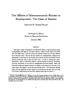
In our scenarios the dynamics are driven only by the demographic transitions in the two economies, and by changes in public policies. Figure 1 presents the paths for population growth and “aging” that we feed into the model (…rst column). Those paths imply the two diagrams in the second column. We present the alternative policy scenarios in subsequent sections. XN /XN
Pop.growth (n) 0.02
h
0.2
f
0.015 0.01
0.15
0.005 0
0.1
-0.005 -0.01 2050
2100
2150
2200
2050
Lif e expect.(y ears)
2100
2150
2200
Dependency ratio
95 0.7 90 0.6 0.5
85
0.4 80
0.3 0.2
75
0.1 70 2050
2100
2150
2200
2050
2100
2150
2200
Figure 1: Demographic trends in Brazil (solid red line) and OECD (dotted blue line)
19
3.2.2
Baseline scenario: Closed economies
Figure 2.1 presents the dynamic paths for various variables in the two economies under the assumption of no trade in goods nor assets. This Baseline closed-economy scenario is our benchmark in this chapter, and henceforth we use Baseline to refer to all scenarios in which the current social security systems remain in place. This is in contrast with subsequent scenarios in which we entertain social security reforms. In the absence of productivity growth and keeping the social security incentives unchanged, aging implies declining paths for GDP and consumption per capita in both economies. The generous public pension system in Brazil drives the associated public expenditures above 25% of GDP in the new steady state, and the required …nancing leads to a dramatic increase in tax revenues, of almost 20% of GDP. Interest rates in Brazil are much higher than in the OECD, in accordance with the di¤erent levels of capital per worker. GDP per capita
Consumption per capita
K per worker
1.5 4
0.6 1
3
0.4 0.5
2 0.2
0
1 2050
2100
2150
2200
2050
2100
2150
2200
2050
2100
2150
2200
Net domest.sav ings(GDP share) 0.05
0
-0.05 2050
2100
2150
2200
Pension pay (GDP share) 0.3
Taxes (GDP share)
Interest rate
0.6 0.1
0.2
0.08 0.4 0.06
0.1
0.04 0
0.2 2050
2100
2150
2200
2050
2100
2150
2200
2050
2100
2150
2200
Figure 2.1: Baseline closed scenario - Brazil (solid red line) and OECD (dotted blue line) In Figures 2.2 and 2.3 we present the paths for the …rst and second demographic dividends, as well as a few other variables that are helpful in understanding the composition e¤ects in the former and the behavioral e¤ects in the latter. Whenever we present separate paths for workers and retirees, solid and dashed red lines correspond to, respectively, Brazilian workers and retirees, while dotted and dash-dot blue lines correspond to, respectively, OECD workers and retirees. 20
The adverse dynamics of the …rst demographic dividend (Figure 2.2, chart (3,1)) are directly implied by the composition e¤ect of demographic developments (Figure 1, chart (2,2)). In terms of the second demographic dividend, prospects are essentially neutral for the OECD, and alternate from slightly positive for many decades (reaching at most 0:20%, for a short time period) to slightly negative in the subsequent decades for Brazil (Figure 2.2, chart (3,2)). This yields a slightly upward hump-shaped pro…le for total consumption per (e¤ective) worker (Figure 2.2, chart (2,2)). But even in the positive phase, the second dividend is not enough to o¤set the negative e¤ect of the …rst dividend, and total consumption per (e¤ective) consumer falls (Figure 2.2, chart (2,1)).
NPV of indiv idual wealth
Indiv idual consumption per period
14 12 10 8 6 4 2
1
0.5
0 2050
2100
2150
2200
2050
T.C./Ef f .Consumer
2100
2150
2200
2150
2200
T.C./Ef f .Worker 1.5
1 0.8
1
0.6 0.5 2050 -3
2100
2150
2200
2050 -3
1st Div idend
x 10
x 10
4
4
2
2
0
0
-2
-2
-4
2100
2nd Div idend(T.C./Ef f .Worker)
-4 2050
2100
2150
2200
2050
2100
2150
2200
Figure 2.2: Baseline closed scenario - Brazil (solid and dashed red lines) and OECD (dotted and dash-dot blue lines) –demographic dividends The two top diagrams of Figure 2.2 shed light on the behavioral e¤ects underlying the second dividend. While in the OECD the net present value (NPV) of workers’wealth is slightly overtaken by retirees’over time (dotted and dash-dot blue lines, respectively, in Figure 2.2, chart (1,1)), in Brazil retirees’wealth increases and workers’wealth decreases (solid and dashed red lines, respectively). In the long run, Brazilian workers own essentially zero assets (Figure 2.3, chart(3,1)), and retirees are the only asset owners (Figure 2.3, chart(3,2)). Retirees consume more than workers in both regions, but over time this di¤erence widens in Brazil (Figure 2.2, chart (1,2)).
21
Wage
NPV human wealth(per worker) 6
1 0.8
4
0.6 2
0.4
0
0.2 2050
2100
2150
2200
2050
PV worker pension(per worker)
2100
2150
2200
PV retiree pension(per retireee)
8
8
6
6
4
4
2
2
0
0 2050
2100
2150
2200
2050
Worker assets(per worker) 6
6
4
4
2
2
0
0
-2
-2 2050
2100
2150
2100
2150
2200
Retiree assets(per retiree)
2200
2050
2100
2150
2200
Figure 2.3: Baseline closed scenario - Brazil (solid and dashed red lines) and OECD (dotted and dash-dot blue lines) –wealth decomposition 3.2.3
Closed vs. sudden opening13
To understand the role of the “closed economy”assumption, in Figures 3.1 and 3.2 we compare the results for Brazil presented in the previous section (dotted black line) with a scenario in which the economies suddenly open up to trade (solid red line) in goods and assets at time zero (i.e., in 2010). Due to the relative size of the two economies, the OECD dynamics are much more similar in the two scenarios (closed and open economies). The reason is that trade and capital ‡ows to and from Brazil are small relative to the size of the OECD block. Hence we only present results for Brazil. Whenever we present separate results for workers and retirees, solid and dashed red lines correspond to, respectively, workers and retirees under the open economy assumption, while dotted and dash-dot black lines correspond to, respectively, workers and retirees under the closed economy assumption.
13
In an extended working paper version we consider scenarios in which the two economies are treated as open from the outset. All of our substantive conclusions go through. Results are available upon request.
22
Consumption per capita
GDP per capita
K per worker 2
0.3 0.5
1.5 0.2
0.4
0.1 2050
2100
2150
2200
1 2050
Net domest.sav ings(GDP share)
2100
2150
2200
Curr.Account(GDP share) 0.1
2050
2100
2150
2200
Net f oreign assets(GDP share) 0
0.05 0 -5
0
-0.1
-0.05
-0.2 2050
2100
2150
2200
Pension pay (GDP share) 0.3
-10 2050
2100
2150
2200
2050
Taxes (GDP share)
2100
2150
2200
Interest rate
0.6 0.1
0.2
0.08 0.4 0.06
0.1
0.04 0
0.2 2050
2100
2150
2200
2050
2100
2150
2200
2050
2100
2150
2200
Figure 3.1: Brazil Baseline - sudden opening (solid red line) x Brazil closed (dotted black line) Opening up the economy leads to an immediate drop in interest rates in Brazil to international levels as foreign capital ‡ows massively into the country (compare charts (3,3) in Figures 2.1 and 3.1). Consumption per capita spikes and domestic savings plummet. Brazil starts to run sizeable current account de…cits, which eventually bring the country’s net foreign asset position to a staggering 5 times GDP.14
14
According to Lane and Milesi-Ferretti (2007), from 1970 to 2011, Brazil’s NFA/GDP has varied in the range of 58% and 15%. In 2010, it was estimated to be 39:8%. It thus appears that the closed economy assumption is a better approximation of the degree of openness of the Brazilian economy –that is why it is our baseline scenario.
23
NPV of indiv idual wealth
Indiv idual consumption per period
8 0.6 6 0.4 4 0.2 2 0 2050
2100
2150
2200
2050
T.C./Ef f .Consumer
2100
2150
2200
2150
2200
T.C./Ef f .Worker 1.5
1 0.8
1
0.6 0.5 2050 -3
2100
2150
2200
2050 -3
1st Div idend
x 10
x 10
4
4
2
2
0
0
-2
-2
-4
2100
2nd Div idend(T.C./Ef f .Worker)
-4 2050
2100
2150
2200
2050
2100
2150
2200
Figure 3.2: Brazil Baseline - sudden opening (solid and dashed red lines) x Brazil closed (dotted and dash-dot black lines) –demographic dividends NPV human wealth(per worker)
Wage
4 0.5 2 0.4 0.3
0 2050
2100
2150
2200
2050
PV worker pension(per worker)
2100
2150
2200
PV retiree pension(per retireee)
4
4
2
2
0
0 2050
2100
2150
2200
2050
Worker assets(per worker)
2100
2150
2200
Retiree assets(per retiree)
4
4
2
2
0
0
-2
-2 2050
2100
2150
2200
2050
2100
2150
2200
Figure 3.3: Brazil Baseline - sudden opening (solid and dashed red lines) x closed (dotted and dash-dot black lines) –wealth decomposition 24
Under the current social security systems, the second demographic dividend in Brazil is more favorable if the economy is relatively closed. A high replacement rate disincentivizes savings. Low interest rates in the case of open economies reinforce this e¤ect. Counting on generous future pensions provided by the government and facing lower interest rates that increase the present value of pensions and human capital, Brazilians consume an even higher share of their income and accumulate fewer assets. The net foreign asset position becomes extremely negative, leading to a huge external imbalance against the OECD. Finally, taxes have to increase dramatically to a¤ord high pensions to a fast-aging population. Many of the results implied by the Baseline scenarios are highly implausible. Some of them have to do with assumptions about the environment, such as the economies turning completely open to trade and foreign investments, which cause huge capital ‡ows. Such negative net foreign asset positions of multiple times GDP would almost certainly not materialize, due to the risks of expropriation and default. Likewise, and perhaps most important, due to the assumption that the generous replacement rate of the Brazilian system will remain constant even though the population will soon start aging fast, all scenarios generate paths for the tax burden that are also incredible. Although this argument is outside the model, an increase in taxes of 20% of GDP would most likely be politically infeasible and create strong incentives for tax evasion through “deformalization”of production activities. The extreme nature of some of the outcomes of the Baseline scenarios motivate our analyses of “reform scenarios”, to which we turn next. 3.2.4
Reform scenarios
We start by looking at the e¤ects of a social security reform that changes the rules governing public pensions in a quite radical way. Speci…cally, we study scenarios in which the government announces that expenditures with public pensions will no longer increase as a fraction of GDP, and the replacement rate have to adjust automatically to balance the budget. We name this a Bold reform. This is, of course, an extreme reform assumption. In particular, it would entail defaulting on “contracts”currently in place. Nevertheless, we believe that this exercise is useful because it highlights the potential e¤ects of social security reforms in a stark way. Subsequently we entertain a more realistic, gradual social security reform. Bold reform We present results for Brazil only, starting with closed economies in Figures 4.1-4.3. Relative to the Baseline closed-economy scenario, in the Bold reform scenario GDP per capita and capital per worker increase signi…cantly. Savings are higher and interest rates drop dramatically –eventually reaching levels that are slightly lower than in the advanced economies (compare charts (3,3) in Figures 2.1 and 4.1). Pension expenditures are essentially capped at their initial level of 10% of the GDP and, as the population ages, the replacement rate falls, reaching 26% in 2200. 25
Consumption per capita
GDP per capita
K per worker 2.5
0.3 2 0.5 0.2
0.4
1.5
0.1 2050
2100
2150
2200
1 2050
2100
2150
2200
2050
2100
2150
2200
Net domest.sav ings(GDP share) 0.05
0
-0.05 2050
2100
2150
2200
Pension pay (GDP share) 0.3
Taxes (GDP share)
Interest rate
0.6
0.1 0.08
0.2 0.4
0.06
0.1
0.04
0
0.02
0.2 2050
2100
2150
2200
2050
2100
2150
2200
2050
2100
2150
2200
Figure 4.1: Brazil closed - Bold reform (solid red line) x Baseline (dotted black line) The reform entails an important shift in the paths of the present value of wealth of workers versus that of retirees (Figure 5.2, chart (1,1), solid red line versus dotted black line for workers, and dashed red line versus dash-dot black line for retirees). This arises mainly from the increase in the net present value of human wealth (Figure 5.3, chart (1,1)), but also because of workers’ increased desire to save for retirement (Figure 5.3, chart (3,1)).
26
NPV of indiv idual wealth
Indiv idual consumption per period
8 0.6 6 0.4 4 0.2 2 0 2050
2100
2150
2200
2050
T.C./Ef f .Consumer
2100
2150
2200
2150
2200
T.C./Ef f .Worker 1.5
1 0.8
1
0.6 0.5 2050 -3
2100
2150
2200
2050 -3
1st Div idend
x 10
x 10
4
4
2
2
0
0
-2
-2
-4
2100
2nd Div idend(T.C./Ef f .Worker)
-4 2050
2100
2150
2200
2050
2100
2150
2200
Figure 4.2: Brazil closed - Bold reform (solid and dashed red lines) x Baseline (dotted and dash-dot black lines) –demographic dividends The second demographic dividend is sizeable in the Bold reform scenario, reaching approximately 0:20% per year for almost …fty years, and remaining above the Baseline closed-economy scenario into the next century. In this comparison it becomes clear that behavioral and general equilibrium e¤ects matter for the magnitude of the second dividend. The increase in the NPV of workers’wealth more than compensates the reduction in the present value of retirees’ wealth, and total consumption per e¤ective consumer is also higher. In the long run, workers and retirees end up with approximately the same per capita consumption (Figure 5.2, chart (1,2)). Next, in Figures 5.1-5.3, we compare the e¤ects of reforming social security and suddenly opening up the economy at the same time (in solid and dashed red lines) against the Baseline closed-economy scenario (in dotted and dash-dot black lines). When the economy opens up and social security is reformed, interest rates drop and capital builds up dramatically. In this scenario, Brazilians eventually face a lower replacement rate than OECD citizens, and have stronger incentives to save for retirement. As Brazil moves into current account surpluses – after a period of extremely large current account de…cits – Brazilians accumulate around 2:8 times the country’s GDP in net foreign assets.
27
NPV human wealth(per worker)
Wage
4 0.5 2 0.4 0.3
0 2050
2100
2150
2200
2050
PV worker pension(per worker)
2100
2150
2200
PV retiree pension(per retireee)
4
4
2
2
0
0 2050
2100
2150
2200
2050
Worker assets(per worker)
2100
2150
2200
Retiree assets(per retiree)
4
4
2
2
0
0
-2
-2 2050
2100
2150
2200
2050
2100
2150
2200
Figure 4.3: Brazil closed - Bold reform (solid and dashed red lines) x Baseline (dotted and dash-dot black lines) –wealth decomposition
Consumption per capita
GDP per capita
K per worker 2.5
0.3 2 0.5 0.2
0.4
1.5
0.1 2050
2100
2150
2200
1 2050
Net domest.sav ings(GDP share)
2100
2150
2200
Curr.Account(GDP share) 0.1
2050
2100
2150
2200
Net f oreign assets(GDP share) 5
0.05
0
-0.05
0
0
-0.1
-5
-0.2 2050
2100
2150
2200
Pension pay (GDP share) 0.3
-10 2050
2100
2150
2200
2050
Taxes (GDP share)
2100
2150
2200
Interest rate
0.6
0.1 0.08
0.2 0.4
0.06
0.1
0.04
0
0.02
0.2 2050
2100
2150
2200
2050
2100
2150
2200
2050
2100
2150
2200
Figure 5.1: Brazil - Bold reform with sudden opening (solid red line) x Baseline closed
28
(dotted black line) The initial sudden fall in the propensities to consume is more than compensated by the increase in the present value of wealth of both workers and retirees, who end up consuming more in the very short run. But as soon as retirees’consumption drops, the second dividend falls below the closed-economy case for a couple of decades, to become (and remain) higher after 2050. Except for a period of high savings between 2030 and 2080, total consumption per e¤ective consumer is signi…cantly higher than when the economy remains closed (including the case in which the social security is reformed). The fact that current retirees enjoy an increase in the NPV of their wealth and loose less consumption with a simultaneous opening of the economy makes one think about the political economy aspects of policies that involve social security reforms and “trade liberalizations”. We return to this issue at the end of this chapter.
NPV of indiv idual wealth
Indiv idual consumption per period
8 0.6 6 0.4 4 0.2 2 0 2050
2100
2150
2200
2050
T.C./Ef f .Consumer
2100
2150
2200
2150
2200
T.C./Ef f .Worker 1.5
1 0.8
1
0.6 0.5 2050 -3
2100
2150
2200
2050 -3
1st Div idend
x 10
x 10
4
4
2
2
0
0
-2
-2
-4
2100
2nd Div idend(T.C./Ef f .Worker)
-4 2050
2100
2150
2200
2050
2100
2150
2200
Figure 5.2: Brazil - Bold reform with sudden opening (solid and dashed red lines) x Baseline closed (dotted and dash-dot black lines) –demographic dividends
29
NPV human wealth(per worker)
Wage
4 0.5 2 0.4 0.3
0 2050
2100
2150
2200
2050
PV worker pension(per worker)
2100
2150
2200
PV retiree pension(per retireee)
4
4
2
2
0
0 2050
2100
2150
2200
2050
Worker assets(per worker)
2100
2150
2200
Retiree assets(per retiree)
4
4
2
2
0
0
-2
-2 2050
2100
2150
2200
2050
2100
2150
2200
Figure 5.3: Brazil - Bold reform with sudden opening (solid and dashed red lines) x Baseline closed (dotted and dash-dot black lines) –wealth decomposition Gradual reform The Bold reform scenarios analyzed previously are useful to illustrate the fact that a meaningful second demographic dividend might be possible in Brazil, especially if the economy opens up as social security is reformed. But that is too extreme a reform, as it essentially amounts to capping pensions as a share of GDP in an economy that will soon embark on a fast aging process. In this section we entertain a more plausible, gradual reform. What stands out in the Baseline scenarios with no reform is not as much the current level of expenditures with public pensions, but their projection as the Brazilian population starts to age fast going forward. Given the extremely high replacement rate of 70%, expenditures with pensions will eventually skyrocket to north of 25% of GDP (e.g. chart (3,2) in Figures 2.1 and 3.1). Hence, we consider scenarios in which the current replacement rate is reduced gradually over a period of 25 years to reach the OECD level of 42% by 2035. We name this the Gradual reform scenario. As before, we start with a comparison of the Baseline scenario with the Gradual reform scenario under the assumption of closed economies (Figures 6.1 and 6.3), followed by a situation in which Brazil implements the gradual reform and opens up to trade in goods and assets (Figures 7.1 and 7.3).
30
Consumption per capita
GDP per capita
K per worker 2.5
0.3 2 0.5 0.2
0.4
1.5
0.1 2050
2100
2150
2200
1 2050
2100
2150
2200
2050
2100
2150
2200
Net domest.sav ings(GDP share) 0.05
0
-0.05 2050
2100
2150
2200
Pension pay (GDP share) 0.3
Taxes (GDP share)
Interest rate
0.6
0.1 0.08
0.2 0.4
0.06
0.1
0.04
0
0.02
0.2 2050
2100
2150
2200
2050
2100
2150
2200
2050
2100
2150
2200
Figure 6.1: Brazil closed - Gradual reform (solid red line) x Baseline (dotted black line) Although there are non-negligible di¤erences relative to the Bold reform case, some of the results under a Gradual reform are similar. The perspective of declining replacement rates going forward creates a strong incentive to save. Even in a closed-economy scenario, interest rates in Brazil decline to essentially international levels. As a share of GDP, pensions and taxes decline initially because of the decreasing replacement rate, and then increase again after 2035 because of the increasing dependency ratio. They stabilize, respectively, around 16% and 37% of GDP.
31
NPV of indiv idual wealth
Indiv idual consumption per period
8 0.6 6 0.4 4 0.2 2 0 2050
2100
2150
2200
2050
T.C./Ef f .Consumer
2100
2150
2200
2150
2200
T.C./Ef f .Worker 1.5
1 0.8
1
0.6 0.5 2050 -3
2100
2150
2200
2050 -3
1st Div idend
x 10
x 10
4
4
2
2
0
0
-2
-2
-4
2100
2nd Div idend(T.C./Ef f .Worker)
-4 2050
2100
2150
2200
2050
2100
2150
2200
Figure 6.2: Brazil closed - Gradual reform (solid and dashed red lines) x Baseline (dotted dash-dot black lines) –demographic dividends The reform increases the NPV of human wealth and reduces the present value of retirees’ pensions relative to the Baseline scenario. The increase in the NPV of workers’wealth more than compensates the e¤ects on retirees’wealth, and total consumption per e¤ective consumer ends up higher. Overall, relative to the Bold reform, this scenario certainly appears more palatable for retirees.
32
NPV human wealth(per worker)
Wage
4 0.5 2 0.4 0.3
0 2050
2100
2150
2200
2050
PV worker pension(per worker)
2100
2150
2200
PV retiree pension(per retireee)
4
4
2
2
0
0 2050
2100
2150
2200
2050
Worker assets(per worker)
2100
2150
2200
Retiree assets(per retiree)
4
4
2
2
0
0
-2
-2 2050
2100
2150
2200
2050
2100
2150
2200
Figure 6.3: Brazil closed - Gradual reform (solid and dashed red lines) x Baseline (dotted and dash-dot black lines) –wealth decomposition If the gradual reform starts at the same time as the economy opens up for trade (Figures 7.1-7.3), interest rates go down and capital accumulates faster in the beginning. After a brief period of large current account de…cits, Brazil eventually moves into mild current account surpluses and accumulates the equivalent of 50% of GDP in net foreign assets. The second dividend, highly positive in the …rst few years, is lower than in the Baseline closed-economy scenario after a while. It then becomes higher again sometime before 2050, and remains higher thereafter. The general equilibrium e¤ects on wages are also signi…cant. This con…rms that taking into account such e¤ects might be important in scenarios in which social security is reformed.
33
Consumption per capita
GDP per capita
K per worker 2.5
0.3 2 0.5 0.2
0.4
1.5
0.1 2050
2100
2150
2200
1 2050
Net domest.sav ings(GDP share)
2100
2150
2200
Curr.Account(GDP share) 0.1
2050
2100
2150
2200
Net f oreign assets(GDP share) 5
0.05
0
-0.05
0
0
-0.1
-5
-0.2 2050
2100
2150
2200
Pension pay (GDP share) 0.3
-10 2050
2100
2150
2200
2050
Taxes (GDP share)
2100
2150
2200
Interest rate
0.6
0.1 0.08
0.2 0.4
0.06
0.1
0.04
0
0.02
0.2 2050
2100
2150
2200
2050
2100
2150
2200
2050
2100
2150
2200
Figure 7.1: Brazil - Gradual reform with sudden opening (solid red line) x Baseline closed (dotted black line) Overall, it appears that the gains from opening up the economy at the onset of the gradual social security reform are not as clearcut as in the Bold reform scenario. Perhaps this is not too surprising. Previously, we highlighted that without reforms the second dividend is likely to be larger if the economy is more closed. In contrast, the Bold scenarios show that opening up to trade might be bene…cial for the prospects of a second demographic dividend if social security is revamped aggressively. Loosely speaking, the Gradual reform scenarios fall in between. Hence opening does not look as attractive a proposition as under an aggressive social security reform.
34
NPV of indiv idual wealth
Indiv idual consumption per period
8 0.6 6 0.4 4 0.2 2 0 2050
2100
2150
2200
2050
T.C./Ef f .Consumer
2100
2150
2200
2150
2200
T.C./Ef f .Worker 1.5
1 0.8
1
0.6 0.5 2050 -3
2100
2150
2200
2050 -3
1st Div idend
x 10
x 10
4
4
2
2
0
0
-2
-2
-4
2100
2nd Div idend(T.C./Ef f .Worker)
-4 2050
2100
2150
2200
2050
2100
2150
2200
Figure 7.2: Brazil - Gradual reform with sudden opening (solid and dashed red lines) x Baseline closed (dotted and dash-dot black lines) –demographic dividends NPV human wealth(per worker)
Wage
4 3
0.5
2 0.4
1
0.3
0 2050
2100
2150
2200
2050
PV worker pension(per worker)
2100
2150
2200
PV retiree pension(per retireee)
4
4
2
2
0
0 2050
2100
2150
2200
2050
Worker assets(per worker)
2100
2150
2200
Retiree assets(per retiree)
4
4
2
2
0
0
-2
-2 2050
2100
2150
2200
2050
2100
2150
2200
Figure 7.3: Brazil - Gradual reform with sudden opening (solid and dashed red lines) x Baseline closed (dotted and dash-dot black lines) –wealth decomposition 35
4
Conclusions
We use a small-scale, two-country, general equilibrium overlapping generations model to study how public policies and di¤erential demographic developments in Brazil vis-a-vis the developed world might interact to produce or prevent a second demographic dividend in Brazil. Our results suggest that, given the current social security system, a small second demographic dividend might arise if Brazil remains relatively closed to trade in goods and assets. Opening up under current social security arrangements turns out to be a losing proposition in that respect. However, scenarios in which the current social security system remains in place produce incredible paths for expenditures with public pensions and taxes as a share of GDP. This is due to the fact that maintaining the very high replacement rates currently in place in Brazil becomes unsustainable as the country starts to age fast in the next couple of decades. To some extent, the average replacement rate in Brazil is high because average income is relatively low. The social security system currently in place aims to provide at least one minimum wage to every retired citizen older than sixty …ve, or a certain pension (also indexed to the minimum wage) determined as a function of former contributions to the social security system. To the extent that the average income in Brazil increases (due to factors not included in our model), the replacement rate will fall somewhat. But along this transition –even if it happens eventually –the disincentives to save will be in place, reducing the scope for a meaningful second demographic dividend. Moreover, given current rules, it appears more likely that expenditures with pensions will become unsustainable, than that Brazil will grow its way out of this liability. Motivated by those results, we entertain reform scenarios, in which growth in expenditures with public pensions is contained. We consider a Bold reform scenario in which public pensions are frozen as a share of GDP, and the replacement rate has to adjust endogenously to balance the budget, and a more gradual reform scenario, in which the replacement rate in Brazil is lowered to the level that prevails in the OECD over a 25-year period. We also interact these reforms with liberalizations that open up the economy to trade in goods and assets. The Bold reform produces a meaningful second demographic dividend in Brazil, irrespective of whether the economy is open or closed to trade. In fact, in that case becoming more integrated with the world economy arguably becomes a winning proposition. That reform scenario is arguably unrealistic, however, since it involves defaulting on “contracts” that are currently in place, given social security rules. Unfortunately, under a more gradual reform, keeping the economy relatively closed might arguably deliver a larger second dividend. While our model brings discipline to a quantitative analysis of some of the macroeconomic e¤ects of the demographic transition in Brazil, it is of course highly stylized. Hence it should only be seen as a guide to richer discussions –and possibly quantitative analyses –that factor in important dimensions that were left out of our framework and policy exercises. Nevertheless, 36
we can always step outside the model to discuss a few important issues and relate our analysis to other contributions in this volume. As Cooper (2013) points out, the Brazilian case does not quite …t the stereotype of other developing economies where demographic developments appear to be much more favorable, and where social security systems are less generous than in richer, more developed economies (see, e.g., Attanasio et al. 2006). In those cases, opening up to trade in goods and assets would appear to be bene…cial in that it would allow those countries (and the developed world as well) to bene…t from the trading opportunities brought about by the di¤erential demographic developments. Younger, poorer countries can bene…t from capital deepening, whereas older, richer countries can bene…t from a higher return on capital, and sustain higher future consumption. In those cases, the issue of whether the countries attracting substantial amounts of capital have the …nancial infrastructure and the institutions to deal with them becomes important (see, e.g., Albrieu and Fanelli 2012 and Ocampo 2013). Here, again, Brazil does not quite …t the stereotype. In comparison with many other developing economies, Brazil has relatively deep …nancial and capital markets (see, for example, De Mello and Garcia 2012). Relative to the issues discussed in the previous paragraph, our analysis suggests that in the case of Brazil other challenges might be more important. For example, our results suggest that opening up with an eye on the gains from trade due to di¤erential demographic developments only makes sense if the country reforms its social security system. In that context, our model abstracts from important challenges that are likely to arise in practice. One important such challenge has to do with the political economy dimension of reform. Almost inevitably, retirees lose, while workers gain. Thus, reform proposals should face stronger opposition as the dependency ratio increases. This reasoning should be informative of reform strategies that have a higher likelihood of success. They should obviously try to be as bold as possible –if they are to spur a meaningful second dividend – but at the same time they have to be gradual to the extent necessary to make reforming feasible. A possible reform satisfying both criteria would be to announce a change in rules to a new “bold regime,” while preserving current rules for those alive (or already participating in the labor market). A quantitative analysis of such a reform is certainly feasible, and appears worth undertaking in future research. In any case, one can ascertain that the political economy reasoning certainly calls for reforming sooner rather than later.
References [1] Albrieu, Ramiro and Jose M. Fanelli (2012), “Asymmetric demography, …nancial development, and global governance,”Buenos Aires: CEDES.
37
[2]
(2013) “On the Macroeconomic and Financial Implications of the Demographic Transition,”Buenos Aires: CEDES.
[3] Attanasio, Orazio, Sagiri Kitao, and Giovanni L. Violante (2006), “Quantifying the E¤ects of the Demographic Transition in Developing Economies,” Advances in Macroeconomics Volume 6, Issue 1 2006 Article 2: 1-44. [4]
(2007), “Global demographic trends and social security reform,” Journal of Monetary Economics 54: 144–198.
[5] Barreto, F. (1997), “Três ensaios sobre reforma de sistemas previdenciários,” Ph.D. Dissertation, EPGE/FGV/RJ. [6] Barreto, F. and L. Oliveira (2001), “Transição para regimes previdenciários de capitalizaçãao e seus efeitos macroeconômicos de longo prazo no Brasil,” Estudos Econômicos 31. [7] Blanchard, Olivier (1985), “Debt, De…cits and Finite Horizons,”Journal of Political Economy, 93: 223-247. [8] Carvalho, José Alberto M. (2004), “Crescimento populacional e estrutura demográ…ca no Brasil,”Belo Horizonte: UFMG/Cedeplar. [9] Cooper, Richard (2013), “Demography, Economic Growth and Capital Flows,” Harvard University, working paper. [10] De Mello, João Manoel P.; Garcia, Márcio G. P. (2012), “Bye, Bye Financial Repression, Hello Financial Deepening: The Anatomy of a Financial Boom,” The Quarterly Review of Economics and Finance 52: 135–153. [11] Ellery Jr., Roberto G.; Bugarin, Mirta N. S. (2003), “Previdência Social e Bem Estar no Brasil,”Revista Brasileira de Economia 57: 27-57. [12] Epstein, Larry and Stanley Zin (1989), “Substitution, Risk Aversion, and the Temporal Behavior of Consumption and Asset Returns: A Theoretical Framework,” Econometrica 57: 937-969. [13] Farmer, Roger (1990), “RINCE Preferences,”Quarterly Journal of Economics 105: 43-60. [14] Ferrero, Andrea. (2010), “A Structural Decomposition of the U.S. Trade Balance: Productivity, Demographics and Fiscal Policy.”Journal of Monetary Economics 57: 478-490. [15] Galor, Oded (2011), “The demographic transition: causes and consequences,” NBER Working Paper, n. 17057. 38
[16] Gertler, Mark (1999), “Government Debt and Social Security in a Life-Cycle Economy,” Carnegie-Rochester Conference Series on Public Policy 50: 61-110. [17] Giambiagi, Fabio and Paulo Tafner (2010), “Demogra…a: a ameaça invisível,” Elsevier: Rio de Janeiro. [18] Imrohoroglu, A., Imrohoroglu, S., & Jones, D. (1995), “A life cycle analysis of social security,”Economic Theory 6: 83-114. [19] IMF (2011), “The Challenge of Public Pension Reform in Advanced and Emerging Economies,”IMF Fiscal A¤airs Department, December 28, 2011. [20] Kreps, David and Evan Porteus (1978), “Temporal Resolution of Uncertainty and Dynamic Choice Theory,”Econometrica 46: 185-200. [21] Krueger, Dirk and Alexander Ludwig (2007), “On the consequences of demographic change for rates of returns to capital, and the distribution of wealth and welfare,” Journal of Monetary Economics 54: 49–87. [22] Lane, Philip R. and Gian Maria Milesi-Ferretti (2007), “The external wealth of nations mark II: Revised and extended estimates of foreign assets and liabilities, 1970–2004,” Journal of International Economics 73: 223-250. [23] Lee, R. D., Lee, Sang-Hyop Lee and Andrew Mason (2008). Charting the economic lifecycle. In A. Prskawetz, D. E. Bloom, &W. Lutz (Eds.), Population aging, human capital accumulation, and productivity growth, a supplement to population and development review 33 (pp. 208–237). New York: Population Council. [24] Mason, Andrew and Ronald Lee (2007), “Transfers, Capital, and Consumption over the Demographic Transition,” In Population Aging, Generational Transfers and the Macroeconomy, edited by Robert Clark, Naohiro Ogawa, and Andrew Mason, pp. 128-162 Cheltenham, UK: Edward Elgar. [25] Mason, A., Lee, R., Tung, A.-C., Lai, M. S., Miller T. (2009). Population aging and intergenerational transfers: Introducing age into national income accounts. In D. Wise (Ed.), Developments in the Economics of Aging (pp. 89–122). Chicago: National Bureau of Economic Research and University of Chicago Press. [26] Ocampo, Jose Antonio (2013), “Emerging Economies and the Reform of the Global Monetary System,”Columbia University, working paper. [27] OECD (2012), “Looking to 2060: Long-term global growth prospects,” OECD Economic Policy Paper Series No. 03, November. 39
[28] Turra, Cassio M., Bernardo L. Queiroz and Eduardo L.G. Rios-Neto. (2011), “Idiosyncrasies of intergenerational transfers in Brazil,”in Population Aging and the Generational Economy: A Global Perspective, edited by Ronald Lee and Andrew Mason, pp. 394-407. Northampton, MA: Edward Elgar Publishing, Inc. [29] United Nations, Department of Economic and Social A¤airs, Population Division (2011), World Population Prospects: The 2010 Revision, Volume I: Comprehensive Tables. T/ESA/SER.A/313. [30] Yaari, Menahem (1965), “Uncertain lifetime, life insurance, and the theory of the consumer,”Review of Economic Studies 32: 137-150.
40