Localized Power Aware Broadcast Protocols with Directional Antennas for Wireless Networks with Practical Models Hui Xu, Manwoo Jeon, Shu Lei, Jinsung Cho1, Sungyoung Lee Department of Computer Engineering, Kyung Hee University, Korea {xuhui, imanoos, sl8132}@oslab.khu.ac.kr,
[email protected],
[email protected]
Abstract We consider broadcast protocols in wireless networks that have limited energy and computation resources. There exist localized power aware broadcast protocols with directional antennas in the literature. They assume, however, impractical models where two nodes can communicate if and only if they exist within their transmission radius. In this paper, we consider practical models for localized power aware broadcast protocols. First, we employ a practical and statistic shadowing model for physical layer where nodes can only indefinitely communicate near the edge of the communication range; for link layer we consider EER (end-to-end retransmission). Second, we employ “Incremental Power with Directional Antennas” philosophy in distributed computing way to construct power aware broadcasting tree. Third, impact of practical models on localized power aware broadcast protocols for wireless networks with directional antennas is analyzed, and based on the analysis result we propose new localized broadcast protocol MPLDBIP for wireless networks with directional antennas. Finally Experimental results show that MPLDBIP outperforms LDBIP under practical models.
1. Introduction In wireless networks which have limited resources such as sensor network, communication ranges are limited, thus many nodes must participate to the broadcast in order to have the whole network covered. The most important design criterion is energy and computation conservation, as nodes have limited resources. The use of directional antennas can reduce the beam width angle to diffuse the radio transmission to one direction and thus provides energy savings and interference reduction. All the protocols that have been proposed for broadcast with directional antennas can be classified into two kinds of solutions: centralized 1
and localized. Centralized solutions mean that each node should keep global network information and global topology. There exist several centralized energy aware broadcast algorithms for the construction of broadcast trees with directional antennas in the literature. In addition, the well-known energy-aware algorithm of Directional Broadcast Incremental Power (DBIP) [1] is “node-based” algorithm and exploits the “wireless broadcast advantage” property associated with directional antennas. Simulation shows that DBIP has very good performance in energy saving. While the problem of centralized approach is that mobility of nodes or frequent changes in the node activity status (from “active” to “passive” and vice-versa) may cause global changes in topology which must be propagated throughout the network for any centralized solution. This may results in extreme and unacceptable communication overhead for networks. Hence, because of the limited resources of nodes, it is ideal that each node can decide on its own behavior based only on the information from nodes within a constant hop distance. Such distributed algorithms and protocols are called localized [2-6]. The existing localized power aware broadcast protocols for wireless networks with directional antennas, however, assume impractical models where two nodes can communicate if and only if they exist within their transmission radius, such as LDBIP [7] (Localized Directional Broadcast Incremental Power). In this paper, we take practical models into consideration. For physical layer, we employ a universal and widely-used statistic shadowing model, where nodes can only indefinitely communicate near the edge of the communication range. For link layer, we consider EER (end-to-end retransmission without acknowledgement) model. Based on above practical models, we improve the reception probability function proposed in [8] and analyze how to choose the transmission radius between transmission nodes and
Dr. Jinsung Cho is the corresponding author.
Proceedings of the IEEE International Conference on Sensor Networks, Ubiquitous, and Trustworthy Computing (SUTC’06) 0-7695-2553-9/06 $20.00 © 2006
IEEE
relay nodes. We show how the practical models effect the selection of transmission radius in power aware broadcast protocols with the trade off between maximizing probability of delivery and minimizing energy consumption. From our analysis, we have derived the optimal transmission range. With mathematic analysis result we propose new localized power aware broadcast protocols MP-LDBIP. Extensive simulation reveals that MP-LDBIP outperforms LDBIP under practical environment. The remainder of the paper is organized as follows: in Section 2, we introduce our system model, including practical physical layer and link layer protocol model. In Section 3 we present improved approximation reception probability and expected energy consumption model. Section 4 presents the impact of practical models on the selection of transmission radius for wireless networks with directional antennas. In Section 5 we propose new localized power aware broadcast protocol MP-LDBIP and present their performance valuation in Section 6. In Section 7, we present our conclusions and future work.
2. System Model 2.1. Physical Layer Model To the best of our knowledge, the published results in broadcasting are based on free-space or two-ray ground propagation models which are simple and ideal physical layer models. However, the received power at certain distance is a random variable due to multi-path propagation effect which is also known as fading effect. In fact, the above two models predict the mean received power at distance. The shadowing model [9] is expected to be more accurate under practical environment. The shadowing model consists of two parts. The first one is known as path loss model which also predicts the mean received power at distance d, denoted by Pr (d) . It uses a close-in distance d 0 as a reference. Pr (d) is computed relative to Pr (d 0 ) as
⎡ Pr ( d ) ⎤ ⎛ d ⎢ ⎥ = − 10 β log ⎜ P ( d ) r 0 ⎝ d0 ⎣ ⎦ dB
⎞ ⎟ ⎠.
(2)
The second part of the shadowing model reflects the variation of the received power at certain distance. It is a log-normal random variable, that is, it is of Gaussian distribution if measured in dB. The overall shadowing model is represented by ⎡ Pr ( d ) ⎤ ⎛ d ⎞ (3) ⎟ + X dB ⎢ ⎥ = − 1 0 β lo g ⎜ ⎣ Pr ( d 0 ) ⎦ d B ⎝ d0 ⎠ ,
where X dB is a Gaussian random variable with zero mean and standard deviation σ dB . σ dB is called the shadowing deviation, and is also obtained by measurement. Eq. (3) is also known as a log-normal shadowing model. The shadowing model extends the ideal circle model to a richer statistic model; nodes can only probabilistically communicate near the edge of the communication range. The use of directional antennas can permit energy savings and reduce interference by concentrating transmission energy where it is needed. We learn from [10] that because the amount of RF energy remains the same, but is distributed over less area, the apparent signal strength is higher. This apparent increase in signal strength is the antenna gain. We use an idealized model in which we assume that all of the transmitted energy is concentrated uniformly in a beam of width θ , as shown in Fig. 1, and then the gain of area covered by the beam can be calculated as θ (4) 2 / (1 − c o s ) 3 6 0
while the gain of the other areas is zero. As a consequence of the “wireless broadcast advantage” property of omni-directional systems [11], all nodes whose distance from Node i does not exceed rij will be able to receive the transmission with no further energy expenditure at Node i.
follows. Pr ( d 0 ) d = ( )β d0 Pr ( d )
(1)
β is called the path loss exponent and is usually empirically determined by field measurement; β = 2 is for free space propagation. Larger values of β correspond to more obstructions and hence faster decrease in average received power as distance becomes larger. Pr (d0 ) can be computed from free space model. The path loss is usually measured in dB. So from Eq. (1) we have
Fig.1. Use of directional antenna While using directional antenna, the advantage property will be diminished, since only the nodes located within the transmitting node’s antenna beam can receive the signal. In Fig. 1, only j, l can receive the signal, while k cannot receive the signal.
Proceedings of the IEEE International Conference on Sensor Networks, Ubiquitous, and Trustworthy Computing (SUTC’06) 0-7695-2553-9/06 $20.00 © 2006
IEEE
We assume that the beam width θ is fixed beam width (e.g θ =30°) and one node can simultaneously support more than one directional antenna. Furthermore, we assume that each antenna beam can be pointed in any desired direction to provide connectivity to a subset of nodes that are within communication range. In addition, we use omni receiving antennas to guarantee the success reception.
⎧ ( dr )2 β ⎪ 1− p(r , d ) = ⎨ 2r −2d 2β ⎪( r ) ⎩ 2
0 ≤d
others
where ȕ is the power attenuation factor with fixed value between 2 and 6, and r is transmission radius with p(r, d=r) = 0.5.
2.2. Link Layer Protocol Model In this section, we look into the link layer and consider separately HHR (hop-by-hop retransmission) where the sender of a packet requires an acknowledgement from receiver and EER (end-to-end retransmission) where the sender of a packet does not. In EER case, the sender sends a packet and the receiver may or may not receive the packet which depends on the reception probability. In HHR case, we incite a link layer communication protocol between two nodes proposed in [8, 12, and 13]. After receiving any packet from sender, receiver sends acknowledgement. If the sender does not receive any acknowledgement, it will retransmit the packet. They also derive the expected number of messages in this protocol as measure of hop count between two nodes. The count includes transmissions by sender and acknowledgments by receiver. They assume both the acknowledgement and data packets are of the same length. In this paper, we only consider EER model. Let S and A be the sender and receiver node respectively, and let |SA| = d be the distance between them. Probability that A receives the packet from S is p(d).
3. Packet Reception Probability and Expected Energy Consumption under Practical Models 3.1. Reception Probability Model In shadowing log-normal model, nodes can only probabilistically communicate near the edge of the communication range. The exact computation of packet reception probability p(d), for use in routing and broadcasting decision, is a time consuming process, and is based on several measurements (e.g. signal strengths, time delays and GPS) which cause some errors. It is therefore desirable to consider a reasonably accurate approximation that will be fast for use. I. Stojmenovic, et al [8, 12, and 13] derives the approximation for probability of receiving a packet successfully as a function of distance d between two nodes. Having in mind an error within 4% the model is
(a) (b) Fig. 2 Reception probability with approximation and modified p(r, d) Fig.2 (a) shows the reception probability with approximation p(r, d) when ȕ is 2 and packet length L is 120. From Fig. 2(a) we can see there are some error results since probability value cannot be larger than 1. The following shows our analysis: ⎧ ( d )2 β ⎧ ( dr )2 β r 0≤ d < r 0 ≤ p ≤ 1 ⎪ 0≤ 1− ≤1 (0≤ d < r) ⎪ 1− 2 >⎨ p ( r , d ) = ⎨ 2 r −2d 2 β 2 − r d 2 β ⎪( r ) ⎪ 0 ≤ ( r ) ≤1 ( d ≥ r ) d ≥r 2 2 ⎩ ⎩
1 ⎧⎪ ⎧⎪ 0 ≤ d ≤ 2 2 β r (0 ≤ d < r) 0≤ d < r => ⎨ ⎨ 1 1 1 2 2 β β ⎪⎩ ( 2 − 2 ) r ≤ d ≤ ( 2 + 2 ) r ( d ≥ r ) ⎩⎪ r ≤ d ≤ ( 2 + 2 2 β ) r While when d increases to 2r, the probability has been zero which means the distance between two nodes has been too far, therefore d should be less than 2r. At last, the modified probability model is ⎧ ( dr ) 2 β 0≤ d < r ⎪ 1− p ( r , d ) = ⎨ 2 r − 2d 2 β ( ) r r ≤d≤ 2r ⎪ 2 ⎩0 o th e r s The figure of our modified approximation p(r, d) when ȕ is 2 is shown in Fig. 2(b).
3.2. Expected Energy Consumption Assume now that two nodes are at distance d, but a packet is sent with transmission radius r and directional beam width θ ; let E represent energy for processing signals at both transmitter and receiver rβ
2π
Proceedings of the IEEE International Conference on Sensor Networks, Ubiquitous, and Trustworthy Computing (SUTC’06) 0-7695-2553-9/06 $20.00 © 2006
IEEE
θ
2π nodes. The exact transmission power is then multiplied by a constant, which is assumed to be 1 for simplicity. Therefore the energy needed by sending node is E + r β θ , while energy at receiving node is E,
for a combined energy 2 E + r β θ . The reception 2π
probability at distance d is p(d)= p(rd/r) = g(d/r), where we defined g(y) = p(r y). In EER link layer model, the sender sends a packet and the receiver may or may not receive the packet, which depends on the probability of receiving. Therefore, the expected energy consumption is θ θ (2E + rβ ) g(d / r) = (2E +dβ (r / d)β )g(d / r) for transmission 2π
2π
between two nodes with directional antenna of beam width θ .
4. Impact of Practical Models Transmission Radius Selection
proposal, we can choose the transmission radius in the scope of [10 15], [20 30] and [30 45] respectively. In Fig. 3(a), the according reception probability is in the scope of [0.5 0.9]; in Fig. 3(b), the according expected energy consumption is in the scope of [53 208], [203 817] and [453 1830], respectively. In summary, for network with directional antenna, we propose to choose the transmission radius in the scope of [d (1/ 5)−1/ 2 β d ] to get the balance between maximizing the probability of delivery and minimizing expected energy consumption.
on
The scenario of our broadcast protocols is as follows: first we construct broadcast tree using power aware broadcast protocols under impractical model; and then choose the optimal transmission radius for every retransmission. As for the metric to decide the optimal transmission radius, there exists a trade off between maximizing probability of delivery and minimizing energy consumption. For network with directional antennas, maximizing probability of delivery will be the primary metric, since transmission coverage overlapping is much less than that in networks with omni-antennas. In EER link layer model, a sender sends a packet and a receiver may or may not receive the packet which depends on the reception probability. The reception probability function is p(r, d) = (1−(d / r)2β /2) for d < r, ((2 r − d ) / r ) 2 β / 2 for r
d, the scope of reception probability is [0.5, 1]; otherwise, if rd) for certain reception probability ¢, we can set get up the formula as 1 − ( d / r )2 β / 2 = α , then r = [2(1 − α )]−1/ 2 β d . Therefore, in order for reception probability to be [0.5 0.9], the transmission radius should be [d (1/ 5)−1/ 2 β d ]. We can verify it through Fig. 3, where ȕ=2, d=10, 20 and 30. According to our
(a) Reception probability
(b) Expected energy consumption Fig. 3 Reception probability and expected energy consumption with fixed distance d.
5. Localized Power Aware Broadcast Protocols with Practical Models In this section, we deal with a localized algorithm for networks with directional-antennas. We name it MP-LDBIP since we extend LDBIP to reflect our analysis under practical model. The goal of the localized algorithm is to allow a localized and distributed computation of broadcast tree. We assume every node knows its local neighbors position information. The principle is as follows: the source node S (the one that initiates the broadcast) computes the broadcast tree with its local neighborhood position information and sends the broadcast packet to each of its one hop
Proceedings of the IEEE International Conference on Sensor Networks, Ubiquitous, and Trustworthy Computing (SUTC’06) 0-7695-2553-9/06 $20.00 © 2006
IEEE
neighbor, while includes N (integer, N>0) hops computed relay information and the Nth hop relay nodes ID in broadcast packet. For each of other nodes, for example, node U who receives the packet for the first time, three cases can happen: 1) The packet contains both relay instructions for U and U’s id. U will use these relay instructions to construct its own local broadcast tree. Then, instead of starting from an empty tree as S did, it extends the broadcasting tree based on what source S has calculated for it. By this way, the joint neighborhood nodes of S and U will use the same spanning tree. 2) The packet contains only relay instructions for U. U will just follow these relay instructions to relay the packet. 3) There are no relay instructions for U. In this case, node U does nothing. After the procedure mentioned above, node U will rebroadcast the packet again to its own one hop neighbor and include N hops computed relay information for its own relay nodes and the Nth hop relay nodes id, just like what source node has done. The reason why we use N to refer relay nodes hop number is that the range within which each node manage positional information on other nodes can be changed according to requirement, and the optimal changes according to the application demands and the node’s hardware performance. In this principle, there may be some nodes which will receive this packet more than one time, then at this time, node can simple drop the packet and doesn’t rebroadcast again. In order to reduce overlap, we use the neighbor nodes elimination scheme. Source node will include its local N hops neighbor nodes in packet, because these nodes certainly will receive the packet soon. Once the node which is in charge of recalculating local spanning tree receives the packet, except recording the relay information it should also record the nodes which will be covered soon. If the covered node is not used in relay information and also is a neighbor node of this node, then this node will delete it from its neighbor list and after deletion calculate its own broadcast tree. Fig.4 is the pseudo-code of MPLDBIP algorithm.
��6HW�XS�EURDGFDVW�SDFNHW�3�� ��,QFOXGH�1�KRSV�UHOD\�LQVWUXFWLRQV�LQ�3�� ��,QFOXGH�1�KRSV�QHLJKERUV′,'�LQ�3�� ��,QFOXGH�1WK�KRS�UHOD\�LQVWUXFWLRQV�LQ�3�� ��6HQG�3�WR�HDFK�RI�LWV�RQH�KRS�QHLJKERU�XVLQJ� GLUHFWLRQDO� DQWHQQD�� WUDQVPLVVLRQ� UDGLXV�VKRXOG� EH� LQ�WKH�VFRSH�RI�>G� (1/ 5)−1/ 2 β d @��ZKHUH� G�LV�GLVWDQFH� EHWZHHQ�WZR�QRGHV�� ��`� ���)RU�DQ\�QRGH�8��H[FHSW�6 �� ���LI�QRGH�8�UHFHLYHV�SDFNHW�3 ^� ����LI�WKH�ILUVW�WLPH ^� �����,QVSHFW�SDFNHW�3�� �����LI�WKHUH�LV�UHOD\�LQVWUXFWLRQ�IRU�8 ^�� ������LI�8′,'�H[LVWV�LQ�1WK�KRS�UHOD\�QRGHV′,' ^� �������5HFRUG�DOO�UHOD\�LQVWUXFWLRQV�IRU�8�� �������
1HLJKERU�1RGHV�(OLPLQDWLRQ�6FKHPH
�� �������&KHFN�LQFOXGHG�FRYHUHG�QRGHV′,'��
�������:KLOH��,'� 8′V�DGGUHVV �,'∉ UHOD\� �������LQVWUXFWLRQ�LQIR � ���� ����
LI��,' ⊂ 8′V�ORFDO�QHLJKERUV�OLVW �
��GHOHWH�WKLV�QRGH�UHFRUG�IURP�8′V�ORFDO� QHLJKERUV�OLVW��
��������
8′V�ORFDO�FDOFXODWLRQ
�� �������5HIHU�UHFRUGHG�UHOD\�LQVWUXFWLRQV�� �������8VH�8′V�PRGLILHG�ORFDO�QHLJKERUV�OLVW�� �������&RPSXWHV�8′V�ORFDO�EURDGFDVW�WUHH�� �������$FW�DV�VRXUFH�QRGH�� ���� � `HOVHLI�8′,'� GRHV� QRW� H[LVW� LQ� 1WK� KRS� UHOD\� QRGHV′,' � ������2QO\�UHOD\�UHFHLYHG�SDFNHW�DV�UHFRUGHG� �UHOD\�LQVWUXFWLRQV�DQG�UHOD\�WUDQVPLVVLRQ� �UDGLXV�VKRXOG�EH�ZLWKLQ�>G� (1/ 5)−1/ 2 β d @�� ���`HOVHLI�WKHUH�LV�QR�UHOD\�LQVWUXFWLRQ�IRU�8 � ������'R�QRWKLQJ��
��5DQGRPO\�VHOHFW�VRXUFH�QRGH�6�
����`HOVH��
��)RU�VRXUFH�QRGH�6��
�����6LPSO\�GURS�SDFNHW�3��
��^��
VRXUFH�QRGH′V�ORFDOH�FDOFXODWLRQ
��
���`
��&RPSXWHV�LWV�ORFDO�EURDGFDVW�WUHH�DV�03�'%,3� GRHV�VKRZQ�LQ�)LJ�����
Fig. 4 Pseudo-code of MP-LDBIP algorithm As for how to calculate broadcast spanning tree with
Proceedings of the IEEE International Conference on Sensor Networks, Ubiquitous, and Trustworthy Computing (SUTC’06) 0-7695-2553-9/06 $20.00 © 2006
IEEE
directional broadcast incremental power principle, a pseudo code of broadcast spanning tree construction can be written as Fig. 5.
propagation model
two ray ground / shadowing
Table 2: Parameters of shadowing model
,QSXW�� JLYHQ� DQ� XQGLUHFWHG� ZHLJKWHG� JUDSK� *�1�$ ��
path loss exponent
2.0
ZKHUH�1��VHW�RI�QRGHV��$��VHW�RI�HGJHV�
Gaussian random variable
zero mean and standard deviation as 4.0db
,QLWLDOL]DWLRQ��VHW�7� ^6`�ZKHUH�6�LV�WKH�VRXUFH�QRGH�RI�
seed for RNG
1
PXOWLFDVW�VHVVLRQ��6HW�3�L � ���IRU�DOO��ื Lื �_1_�ZKHUH�
reference distance
1.0m
3�L �LV�WUDQVPLVVLRQ�SRZHU�RI�QRGH�L��
�L�N
The wireless network is composed of 100 nodes randomly placed in a square area which size is changed to obtain different network density D, which is defined as the average number of neighbors per each node using the unit graph model. The formula can be written as: π r2 (5) D = N *
SRZHU� ΔPij d α θ f �3�L ��RWKHUZLVH�� ΔPij d α θ f ��� ij ij 2π 2π G�LV�WKH�GLVWDQFH�EHWZHHQ�WZR�QRGHV��
where A represents the edge length of deployment square area, and r is the maximum transmission range. From Eq. (5), we can calculate N π (6) A = r
3URFHGXUH��� ZKLOH�_7_�ำ �_1_� GR�ILQG�DQ�HGJH��L�M ∈ 7 × �1�7 �ZLWK�IL[HG�EHDP� ZLGWK� θ f �VXFK�WKDW� ΔPij �LV�PLQLPXP�� LI� DQ� HGJH�
∈ 7 × 7� UDLVLQJ� WKH� OHQJWK� UDQJH� RI� EHDP� FDQ� FRYHU� D� QRGH� M ∈ �1�7 �� WKHQ� LQFUHPHQWDO�
DGG�QRGH�M�WR�7��L�H���7�� �7 ∪ ^M`�� VHW�3�L �� �3�L ��� ΔPij �
Fig. 5 Pseudo code of broadcast tree construction
6. Performance Evaluation 6.1. Simulation Parameters We use ns2 as our simulation tool and assume AT&T's Wave LAN PCMCIA card as wireless node model which parameters are listed in Table 1. As for system model, we employ EER model for link layer and 802.11 MAC protocol, and in physical layer we apply two ray ground model as the impractical propagation model, and shadowing model as practical propagation model. Table 2 shows parameters of shadowing model. Table 1: Parameters for wireless node model frequency
2.4GHZ
maximum transmission range
40m
maximum transmit power
8.5872e-4 W
receiving power
0.395 watts
transmitting power omni-antenna gain of receiver/transmitter fixed beam width of directional antennas directional antenna receiver/transmitter gain MAC protocol
0.660 watts 1db 30 58.6955db
A
D
2
,
.
For each measure, 50 broadcasts are launched and a new network is generated for each broadcast. The RAR (Reach Ability Ratio) is the percentage of nodes in the network that received the message. Ideally, each broadcast can guarantee 100% RAR value. While in practical environment since nodes can only indefinitely communicate near the edge of the communication range, RAR may be less than 100% and then RAR becomes more important in performance evaluation for broadcast protocols. To compare the different protocols, we observe the total power consumption over the network when a broadcast has occurred. We compute a ratio named ECR, that represents the energy consumption of the considered protocol compared to the energy that would have been spent by a blind flooding (each node retransmits once with maximum transmission range). The value of ECR is so defined by: E p r o to c o l (7) ECR =
E
× 1 0 0.
flo o d in g
We also observe the SRB (Saved Rebroadcast) which is the percentage of nodes in the network that received the message but did not relay it. A blind flooding has a SRB of 0%, since each node has to retransmit once the message. In practical environment even some nodes are chosen as relay nodes, it’s possible that they do not relay packets since they have not received packets successfully. Therefore especially in practical models the SRB is an important measure for performance evaluation.
802.11
Proceedings of the IEEE International Conference on Sensor Networks, Ubiquitous, and Trustworthy Computing (SUTC’06) 0-7695-2553-9/06 $20.00 © 2006
IEEE
6.2. Performance Evaluation for MP-LDBIP under Practical Environment In this section, we present our performance evaluation for the schemes proposed above. For network with directional antenna, we propose to choose the transmission radius in the scope of [d (1/ 5)−1/ 2 β d ] to maximize the probability of delivery. In our simulation, since we set the path loss exponent ȕ as 2.0, the appropriate transmission scope for MPLDBIP is [d 1.5d].
Fig.6. RAR comparison for MP-LDBIP with different transmission radius
Fig.6-8 shows the performance of MP-LDBIP when transmission radius r varies within [d 2d] where d is the distance between two nodes. In particular, when r/d=1 (r=d), MP-LDBIP is LDBIP. In Fig. 6 we can find that the RAR of LDBIP under shadowing model is zero, which demonstrates the necessary of our proposal of increasing the length of transmission radius. When network density is 80 or 90, r≥1.1d can already supply acceptable RAR (larger than 50%); when network density is 60 or 70, r≥1.3d can start to supply acceptable RAR. In Fig. 7 we can see as r/d value raises, i.e. transmission radius increases, the ECR value also raises. Therefore if r is chosen within the range of [1.1d 1.5d] for D=80 or 90 and [1.3d 1.5d] for D=60 or 70, we can get high enough RRA value and low enough ECR value. Above simulation result shows our proposed range of [d (1/ 5)−1/ 2 β d ] is the appropriate transmission radius scope. SRB is percentage of saved retransmission. If SRB decreases, it means there are more nodes participating retransmission which will spend more energy. In Fig. 8 we can see as r/d value raises, the SRB value also raises. Therefore if r is chosen within the range of [1.1d 1.5d] for D=80 or 90 and [1.3d 1.5d] for D=60 or 70, we can get high enough RRA value and high enough SRB value. Above simulation result proves again our proposed MP-LDBIP outperforms LDBIP under practical models.
7. Conclusions
Fig.7. ECR comparison for MP-LDBIP with different transmission radius
To the best of our knowledge, this is the first work that considers the impact of practical physical layer and link layer model on localized power aware broadcast protocols with directional antennas. We investigated localized broadcast protocols without acknowledgements and presented the trade off between maximizing probability of delivery and minimizing energy consumption for wireless networks with practical models. We show how the practical models effect the selection of transmission radius in localized broadcast protocols in network with directional antenna. We propose new power aware broadcast protocols: Maximizing Reception Probability Protocols for networks with directional antennas (MP-LDBIP). The performance of the proposed algorithm has been evaluated and compared. The experiment results show that MP-LDBIP outperform LDBIP under practical environment.
Fig.8. SRB comparison for MP-LDBIP with different transmission radius
Proceedings of the IEEE International Conference on Sensor Networks, Ubiquitous, and Trustworthy Computing (SUTC’06) 0-7695-2553-9/06 $20.00 © 2006
IEEE
Acknowledgement This work was supported by grant No. R01-2005-00010267-0 from Korea Science and Engineering Foundation in Ministry of Science and Technology.
References [1] J.E. Wieselthier, G.D. Nguyen and A. Ephremides, “Energy-Limited Wireless Networking with Directional Antennas: The Case of Session-Based Multicasting”, Proc. IEEE INFOCOM, 2002, pp. 190-199. [2] P. Bose, P. Morin, I. Stojmenovic and J. Urrutia, “Routing with guarantee delivery in ad hoc networks”, ACM/Kluwer Wireless Networks, 2001, pp. 609-616. [3] T. Chu and I. Nikolaidis, “Energy efficient broadcast in mobile ad hoc networks”, In Proc. Ad-Hoc Networks and Wireless, Toronto, Canada, 2002, pp. 177-190. [4] W. Peng and X. Lu, “On the reduction of broadcast redundancy in mobile ad hoc networks”, In Proc. Annual Workshop on Mobile and Ad Hoc Networking and Computing (MobiHoc'2000), Boston, Massachusetts, USA, 2000, pp. 129-130. [5] A. Qayyum, L. Viennot and A.Laouiti, “Multipoint relaying for flooding broadcast messages in mobile wireless networks”, In Proc. 35th Annual Hawaii International Conference on System Sciences, Hawaii, USA, 2002 [6] J. Wu and H. Li, “A dominating-set-based routing scheme in ad hoc wireless networks”, In Proc. 3rd Int'l Workshop Discrete Algorithms and Methods for Mobile Computing and Comm, Seattle, USA, 1999, pp. 7-14. [7] Hui Xu, Manwoo Jeon, Lei Shu, Wu Xiaoling, Jinsung Cho and Sungyoung. Lee, “Localized Energy-aware Broadcast Protocol for Wireless Networks with Directional Antennas”, International Conference on Embedded Software and Systems, 2005, pp. 696-707. [8] I. Stojmenovic, A. Nayak, J. Kuruvila, F. OvalleMartinez and E. Villanueva-Pena, “Physical layer impact on the design of routing and broadcasting protocols in ad hoc and sensor networks”, Journal of Computer Communications (Elsevier), Special issue on Performance Issues of Wireless LANs, PANs, and Ad Hoc Networks, 2004. [9] Network Simulator - ns-2, http://www.isi.edu/nsnam/ns/. [10] Joseph J. Carr, “Directional or Omni-directional Antenna”, Joe Carr's Receiving Antenna Handbook, Hightext, 1993. [11] J.E. Wieselthier, G.D. Nguyen and A. Ephremides, “Algorithms for Energy-Efficient Multicasting in Static Ad Hoc Wireless Networks”, Mobile Networks and Applications (MONET), 2001, vol. 6, no. 3, pp. 251-263. [12] Johnson Kuruvila, Amiya Nayak and Ivan Stojmenovic, “Hop count optimal position based packet routing algorithms for ad hoc wireless networks with a realistic physical layer”, IEEE Journal on selected areas in communications, 2005. [13] J. Kuruvila, A. Nayak and I. Stojmenovic, “Greedy localized routing for maximizing probability of delivery in wireless ad hoc networks with a realistic physical layer”, Algorithms for Wireless And mobile Networks (A_SWAN) Personal, Sensor, Ad-hoc, Cellular Workshop, at Mobiquitous, Boston, 2004, pp. 22-26.
Proceedings of the IEEE International Conference on Sensor Networks, Ubiquitous, and Trustworthy Computing (SUTC’06) 0-7695-2553-9/06 $20.00 © 2006
IEEE