Localized Geographic Routing to a Mobile Sink with Guaranteed Delivery in Sensor Networks Xu Li, Jiulin Yang, Amiya Nayak, Senior Member, IEEE, and Ivan Stojmenovic, Fellow, IEEE
Abstract—We propose a novel localized Integrated Location Service and Routing (ILSR) scheme, based on the geographic routing protocol GFG, for data communications from sensors to a mobile sink in wireless sensor networks. The objective is to enable each sensor to maintain a slow-varying routing next hop to the sink rather than the precise knowledge of quick-varying sink position. In ILSR, sink updates location to neighboring sensors after or before a link breaks and whenever a link creation is observed. Location update relies on flooding, restricted within necessary area, where sensors experience (next hop) change in GFG routing to the sink. Dedicated location update message is additionally routed to selected nodes for prevention of routing failure. Considering both unpredictable and predictable (controllable) sink mobility, we present two versions. We prove that both of them guarantee delivery in a connected network modeled as unit disk graph. ILSR is the first localized protocol that has this property. We further propose to reduce message cost, without jeopardizing this property, by dynamically controlling the level of location update. A few add-on techniques are as well suggested to enhance the algorithm performance. We compare ILSR with an existing competing algorithm through simulation. It is observed that ILSR generates routes close to shortest paths at dramatically lower (90% lower) message cost. Index Terms—Geographic routing, location service, localized algorithms, mobile sink, wireless sensor networks.
I. I NTRODUCTION
W
IRELESS sensor networks (WSNs) are a cooperative environment where resource-constrained sensors monitor their surroundings and report to a predefined data sink through message relay. In the presence of sink mobility, it is too expensive for sensors to learn and maintain the knowledge of accurate sink location or rely on network-wide flooding for routing to the sink. A practical routing algorithm must be scalable to potentially large network size and efficient in bandwidth and energy usage. Localized algorithms, where simple local behavior achieves desired global objective, offer both scalability and efficiency. In many WSN applications, a reported event, is meaningful and can be responded to only if its position is known. Effective localization methods [7] have been developed. We reasonably assume the availability Manuscript received January 8, 2011; revised July 09, 2011; accepted August 30, 2011. This work was partially supported by NSERC CRDPJ 386874-09 (Reliable and secure QoS routing and transport protocols for mobile ad hoc networks) and NSERC STPSC 356913-2007 (Maintaining fault-tolerant networks of robots for supporting wireless sensor networks). X. Li is with INRIA Lille - Nord Europe, Parc scientifique de la haute borne, Villeneuve d’Ascq 59650, France (email:
[email protected]). J. Yang, A. Nayak, and I. Stojmenovic are with the School of Information Technology and Engineering, University of Ottawa, Ottawa, Ontario K1N 6N5, Canada (email:
[email protected],
[email protected],
[email protected]).
of geographic location to sensors, which then enables positions of sender, destination, and neighbors to forwarding nodes. In this article, we address the problem of geographic routing to a mobile sink in static WSNs through location service approaches. The purpose of having a mobile sink is, for example, for energy-efficient data collection [8]. Since geographic routing requires the knowledge of location of destination, it includes as part of its statement location service, which deals with how to update and search latest location of destination (sink). In the past, location service [9] and geographic routing [10] have been studied in depth mostly as separate problems for wireless ad hoc networks. There are two basic solutions to the routing problem, loosely-coupled and integrated. A loosely-coupled solution divides routing into two stages. At the first stage, source searches for the latest location of the sink by a location service algorithm. In most cases the search ends at a node that either is the sink itself or knows up-to-date sink location, followed by report from that node back to the source, containing the exact position of the sink. Since source location can be included in the search message, this report can be carried by a geographic routing task. At the second stage, a geographic routing algorithm is run to build a path between source and the sink using discovered sink location. This solution may generate large message overhead due to lack of joint optimization of the two closely-related sub-problems. The fact that sensors share the sink as common destination can be exploited for designing a better protocol. An integrated solution intends to let every node maintain an approximate, rather than the exact, location of the sink. Sink distributes its initial position to every node in the network; later when necessary, it updates location only to a selected subset of nodes. Source may use currently available, but possibly inaccurate, information on sink location and route immediately toward that location, hoping that the position information would become more accurate as the message approaches region containing the sink. Intuitively, this solution has less cost than loosely-coupled solution, if sink information at each node is sufficiently accurate. Only a few such algorithms were presented in literature. They are inferior to the algorithm proposed here for high message cost and/or lack of delivery guarantee. A survey of these algorithms can be found in [8]. A. Problem statement We consider a connected WSN with a mobile sink. Nodes (sensors and the sink) have the same transmission range R. Any two nodes can communicate directly as long as their separation is not larger than R. The network is therefore
modeled as unit disk graph (UDG). Nodes are aware of their own geographic position by attached GPS device or some localization algorithm, and the locations of 1-hop neighbors via ‘hello’ message. By listening to ‘hello’ message, sink is able to identify incidental link creation and breakage. ‘Hello’ frequency has obvious impact on routing performance. We assume a ‘hello’ protocol adaptive to sink mobility for timely neighborhood update so as to focus on the routing problem. Sensors are assumed static here for simplicity, although the same algorithms can be applied if they are moving slowly. They are assumed to be connected without the sink (this assumption is needed for guaranteed delivery property). Sink initially floods (once) the network with its location. Then it moves slowly at a speed small enough for detecting neighborhood change and always remains connected to the network, i.e., within at least one sensor’s transmission range. Sink mobility is classified as unpredictable or predictable. Unpredictable movement is obtained by attaching sink on a mobile entity, e.g., an animal, which has unknown behavior to the network. Sink may move at random and has no knowledge of its own mobility. It reports its current position to sensors when necessary; sensors route packets to the reported position. In predictable (controllable) movement, sink is placed on a mobile platform such as robot. It moves step by step, each step straightly toward a location called endpoint. Sink knows its current step endpoint and the time needed to reach that point, and reports this information to sensors. It may start a new step to a different endpoint occasionally, even before finishing current one. Assuming delay tolerance, sensors buffer packets and route them to the reported endpoint after sink arrives there. The average dilation (also known as stretch factor) of a routing algorithm is the average ratio of hop count of discovered route to hop count of shortest path. Having a low average dilation is only useful if the delivery rate (i.e., the ratio of number of successfully delivered packets to number of generated packets) of the algorithm is high [2]. The goal in this article is to develop an integrated location service within GFG routing [2] for guaranteed packet delivery (delivery rate = 1) to the sink with low average dilation at minimal overhead. B. Our contributions We propose a novel Integrated Location Service and Routing scheme ILSR for the above stated problem. This scheme incorporates the well-known GFG routing protocol [2] (which guarantees delivery in static networks [5]) with two types of location update, flooding type and routing type, to deal with sink mobility. Flooding-type location update is restricted only within necessary area, where nodes experience (next hop) change in GFG routing to the sink, and its coverage area is not determined by the sink but defined by nodal local decision on retransmission. Routing-type location update is engaged to prevent routing failure. It is destined to some particular destinations, identified by certain policies, and carried out by a uni-casting or multi-casting task. We consider both unpredictable (UM) and predictable (CM) sink mobility and present two versions, i.e., ILSR-UM and ILSR-CM. In ILSR-UM, sink initiates flooding-type loca-
tion update after incidental link breakage occurs. In ILSRCM, it predicts incidental link breakage and performs such location update before that happens. In both versions, sink also acts whenever it discovers incidental link creation. The two versions differ in routing-type location update too. In ILSR-UM, sink sends dedicated location update message to newly disconnected neighbors that are possibly out of range of flooding-type location update. In ILSR-CM, it sends such message to the old endpoint before endpoint change so that message destined to that point can be rerouted. We formally prove that ILSR (both versions) guarantees packet delivery in WSNs modeled as UDG. This property is preserved even if nodes do not retransmit flooding-type location update message. Thus we may achieve desired tradeoff of message cost and average dilation by restricting the number of retransmissions of such message to a maximum value. This maximum value is locally computed by the sink according to its own mobility on the fly, through the doubling circle method [1] (referred to as DC in this article). The idea is to define a set of circles with doubling radii and centered at the sink’s initial position, and when the sink moves out a circle, to move the circle to the sink’s current position and set the location update level limit to the radius of the circle. In addition, we propose to apply several addon techniques including connected dominating set (CDS) [3], beaconless location update and intermediate step endpoints for performance improvement. We compare ILSR with the known doubling circle routing and location service algorithm DC [1] through extensive simulation. It is observed that ILSR has dramatically better performance in all tested network scenarios. Compared with their DC counterparts, ILSR-UM with dynamic level control has about 90% less message cost and nearly equal (< 0.1 larger) average dilation, and ILSR-CM has over 90% less message cost and comparable (< 1 larger) average dilation. If no level control is used, both versions will have smaller average dilation than DC while saving around 30 − 70% message cost. Note that ILSR-CM shows inferior dilation performance to ILSR-UM in our simulation. It is because the ILSR-CM variant relies on reported sink mobility (step endpoint) for routing, which may however change unexpectedly. Our simulation results also indicate that our suggested enhancement techniques effectively improve the algorithm performance. II. ILSR FOR UNPREDICTABLE MOBILITY We first present ILSR-UM and prove its correctness. ILSRUM does not rely on any knowledge of sink mobility, and is thus a generic algorithm applicable to arbitrary scenarios including predictable sink mobility. In ILSR-UM, sink monitors its radio connection to neighboring sensors by listening to their ‘hello’ message. It considers a newly disconnected node lost neighbor if that node is not neighboring any of its current one-hop neighbors, or semi-lost neighbor otherwise. A current (one-hop) neighbor covering a semi-lost neighbor is called relay neighbor. Sink is able to classify neighbors because it collects their position. Sink may perform two types of location update, flooding type and routing type, by sending location update message in
(a) UM version Fig. 1.
(b) CM version
Sink location update in ILSR
different ways. Location update message (whether of flooding type or of routing type) is stamped, e.g., by a sink-maintained monotonically increasing sequence number, for distinction and for reflecting freshness. Duplicated or stale message is discarded. For simplicity, we will ignore such message below. Whenever an incidental link breakage or creation occurs, sink transmits a location update message. The message contains the sink’s latest location and a relay list. The relay list contains a smallest subset of rely neighbors that cover all semi-lost neighbors. It is empty in the case of no semilost neighbors. Sink determines the relay list by neighbor designating method MPR [11]. Coverage area of flooding-type location update message is decided by the local retransmission decisions of receiver nodes. A node retransmits such message if and only if either its current next hops to the new and the last reported positions of the sink are different according to GFG (based on Gabriel Graph), or it is in the relay list. In parallel to flooding-type location update, sink may or may not perform routing-type location update. Sink performs such location update if and only if there are lost neighbors. During this process, it sends to lost neighbors a dedicated location update message carrying its latest location. If there is only one lost neighbor, the message will be routed by GFG (uni-casting version). If multiple such neighbors exist, it will be routed by the multi-casting version [14] of GFG. Since lost neighbors are normally near each other, engagement of multi-casting instead of separate routing tasks reduces message overhead. Routing-type of location update is necessary for ILSRUM to provide guaranteed delivery, because lost neighbors could be out of range of flooding-type location update. A node ‘overhears’ a message if it is not the intended receiver but receives the message. Optionally, each node converts an overheard routing-type location update message to floodingtype and handles it as regular flooding-type location update. Figure 1(a) illustrates how ILSP-UM works. Sink moves from position Ai to position Ai+1 . At Ai+1 , it recognizes lost neighbor b, semi-lost neighbor a, and relay neighbor d (covering semi-lost neighbor a), and transmits a floodingtype location update message and a routing-type location update message destined to b. Node c retransmits the received flooding-type message because its next hop to the sink changes according to GFG; d retransmits because it is a selected relay neighbor. Both nodes a and e receive the message from d, and decide to retransmit because of change of routing next hop. f
receives the message forwarded by e; but it does not retransmit because its next hop to the sink remains unchanged. The propagation of the flooding-type location update message finally stops at f , as shown by solid arrowed lines. The routing-type message travels along the path indicated by the dashed arrowed line and reaches destination b. Node h overhears this message from g and converts it to a flooding-type message. But it does not retransmit the message because its next hop to the sink does not change. In this case, it does not matter whether h stores the new location of the sink. Each node drops received duplicated location update messages (which are not shown). L EMMA 1: Suppose that sink performs location update successively at positions Ai and Ai+1 (i ≥ 0). In ILSR-UM applied on a connected network, a sensor with the information of Ai can always route to a sensor that is aware of Ai+1 . Proof: When a sensor u with the (position) information of Ai routes a packet to the sink using GFG algorithm (based on Gabriel Graph), it is guaranteed that a node closest to Ai , say wi , will receive the packet [12]. We refer this property as closest delivery. There are three cases regarding wi : 1) wi is a neighbor of Ai+1 , as node d in Fig. 1(a). In such case, wi will get information of Ai+1 directly from sink. 2) wi is not a neighbor of Ai+1 , but has a neighbor neighboring Ai+1 , as node a in Fig. 1(a). In such case, wi was a semi-lost neighbor when the sink was at Ai+1 , and it must have learnt Ai+1 from flooding-type location update message retransmitted by a relay node. 3) wi is neither a neighbor of Ai+1 nor has a neighbor neighboring Ai+1 , as node b in Fig. 1(a). In such case, wi will get information on Ai+1 from routing-type location update message destined to it. In any of the above cases, wi learns about Ai+1 . During the routing to Ai , before arriving at node wi , packets may also reach a node that already has the information of Ai+1 . Thus u can always route packets to a sensor aware of Ai+1 . T HEOREM 1: In a connected sensor network modeled as unit disk graph, ILSR-UM algorithm provides guaranteed message delivery from any sensor to the mobile sink that is always connected to the network. Proof: Suppose that sink performs location updates successively at positions of A1 , · · · , Ak and its initial position is A0 and current position is Ak . Because sink initially floods the network with its location, every sensor knows about A0 (see Sec. I-A). Suppose that sensor u knowing the position information of Ai (0 ≤ i ≤ k) sends a packet to the sink. According to Lemma 1, it always can route toward Ai through a node, say wi , that is aware of the position of Ai+1 . Then the packet will be directed to Ai+1 from there. Thus the advance toward Ai+1 is made, and iteratively further advances can also be made. Thus, the packet will be directed to a node wk that has the information on Ak . This node will route by GFG the packet to the sink, which is guaranteed to receive the packet as it is connected to the network. III. ILSR
FOR PREDICTABLE MOBILITY
We now present ILSR-CM for delay-tolerant networks by assuming and making use of predictable sink mobility. As in
ILSR-UM, sink may perform flooding-type and routing-type location updates. Location update message is stamped so that duplicated or stale message can be discarded. ILSR-CM differs from ILSR-UM in when location update is performed and in where routing-type location update is destined. Every time when a ‘hello’ message is received, sink predicts which of its incident links will be broken and when, based on the locations of neighbors, and its own location and mobility pattern (speed and acceleration). Right before the link breakage occurs, it transmits a flooding-type location update message carrying its current step endpoint. It transmits such a message also when a new neighbor is discovered. A node retransmits a received flooding-type location update message only if the node’s current next hops (based on GFG) to the new and previously reported positions are different. While relocating to the current step endpoint, sink may decide to move to a different endpoint. In this case, nodes without information of new endpoint will keep routing toward the old endpoint, ending up with routing failure. A technique similar to home-based location service [13] and data-centric storage [12] is used to overcome this problem as follows. Sink performs routing-type location update before changing endpoint, toward the old endpoint using GFG. Any node overhearing a routing-type location update message treats and handles the message as flooding-type one. By the closest delivery property of GFG, the node closest to that point is guaranteed to receive the information. This node is called anchor node. If it later receives packets routed to this old endpoint, it will reroute them to the new endpoint. The only routing control information stored on an anchor node are the old and new endpoint locations and sink arrival time. Packets may be redirected to the new endpoint by an intermediate node with updated information before reaching the anchor node. Anchor nodes form a routing backbone and are responsible for rerouting in case of endpoint change. However, the routing backbone may lead to long zigzag routing paths when used. To overcome this problem, each anchor node sets a flag in its redirected data packets. By seeing this flag, sink knows that a packet has possibly gone through a long zigzag route over the routing backbone, and then sends a routing-type location update message destined to the source node by GFG. Here, if multiple such source nodes are identified at the same time, the multi-casting version of GFG [14] shall be used. Figure 1(b) illustrates how ILSP-CM works. Sink aims at endpoint Ai+1 from Ai . When it reaches location B (where direct connection to node u is about to be lost), it transmits a flooding-type location update message. At location C, it changes its endpoint to Ai+2 and routes this change to Ai+1 (indicated by solid arrowed line), and the anchor node w receives the message. Later, sensor u routes data toward Ai+1 ; the data is received by w. Node w sets a flag in the message and redirects it to Ai+2 , which is the sink’s current endpoint. Having reached Ai+2 , the sink receives the message, sees the flag, and sends a routing-type location update message to u. This process is now shown in the figure though. T HEOREM 2: Suppose that sink always keeps connected to the network. ILSP-CM algorithm provides guaranteed delivery in any connected sensor network modeled as unit disk graph.
Proof: Suppose sink has changed directions several times, to endpoints A1 , A2 , · · · , Ak respectively. Its initial position is A0 and current endpoint is Ak . Every sensor receives one endpoint position, initially A0 or one of later positions. Suppose sensor u knowing the position of Ai (0 ≤ i ≤ k) sends a packet to the sink. By the closest delivery property of GFG, the message arrives to node wi closest to Ai . If i = k, then the sink is or will arrive at Ai which is neighboring wi by the connectivity assumption, and message will be delivered from wi to the sink positioned at Ai . If i < k, then the sink, when it was moving toward Ai+1 , sent routing-type location update message toward Ai by the algorithm, informing about the new step endpoint. By the closest delivery property of GFG, node wi closest to Ai among all sensors, obtained the position of Ai+1 from the sink. The data packet from u will also be routed to wi , where it will be redirected to Ai+1 after arrival. Thus the advance toward Ak is made, and iteratively further steps can also be made. Eventually, the packet will be forwarded to a node wk closest to the current endpoint Ak , which forwards the packet to the sink. Note that a packet routed to Ai may be redirected to more recent Aj (j > i) by any intermediate node knowing the position of Aj . IV. L OCATION UPDATE
LEVEL CONTROL
From the proof of Lemma 1, in ILSR-UM the node wi closest to location Ai gets updated sink location either directly from Ai+1 , or from a relay node one-hop away from Ai+1 , or from a routing-type location update message designated to it. Flooding-type location update message (sent by nodes with different next hops toward new and old sink locations) was not mentioned or used in the proof for providing guaranteed delivery. ILSR-CM uses only such type of location updates, which, from the proof of Theorem 2, does not affect any condition for achieving delivery guarantee. Summarizing, we have the following important corollary. C OROLLARY 1: The guaranteed delivery property of ILSR is not affected by the application (or lack of application) of flooding-type location update message by nodes whose next GFG hop toward new and old sink locations differ. According to this corollary, the message cost of ILSR can be greatly reduced by controlling the level of location update, i.e., the number of retransmissions of a flooding-type location update message, and its delivery guarantee still remains. We denote by LC the maximum location update level allowed. Its minimum value is 0, meaning no retransmission. It is not a predefined parameter, but computed locally by the sink on the fly according to its own mobility. Specifically, the sink executes the doubling circle algorithm DC [1] virtually (without sending any message) while running ILSR. The output of DC is two circles C(t) and C(t + 1), whose radii are respectively 2t R and 2t+1 R, to be flooded for location update. The value of t varies dynamically as the sink moves. Each time when the sink wants to start a flooding-type location update according to ILSR, it sets the level limit to 2t+1 . Location update level control can then be implemented by adding a TTL (Time To Live) field, initially equal to LC, in each flooding-type location update message,
which is decremented during each retransmission. A receiver retransmits the message only if TTL is larger than 0. Location update level control may increase inaccuracy in forwarding information at some nodes and possibly leads to degraded routing performance on average dilation. Its impact on the performance will be shown in Sec. VI via simulation. V. E NHANCEMENT TECHNIQUES In ILSR-UM, message overhead may be reduced if sink is able to apply larger transmission radius than sensors. For example, retransmissions of sink-selected relay nodes in flooding-type location update can be removed, without jeopardizing the guaranteed delivery property, if the transmission radius of sink is at least twice as large as sensors’. However we will pursue other methods. We propose to use a connected dominating set (CDS) as communication backbone, and only let dominating nodes participate in some protocol decisions. A set is dominating if each node either belongs to the set or has a neighbor in it Use of CDS saves message transmissions, especially in largedegree networks. We denote CDS-based ILSR by CDS-ILSR. In CDS-ILSR, a CDS is established spontaneously and locally by the generalized self-pruning rule [3]; only dominating nodes retransmit flooding-type location update messages. The operation of protocol GFG changes a bit as well, as in [4]. Face routing mode is applied to dominating nodes only, that is, face traversal is performed on the planar graph constructed using dominating nodes. Greedy mode remains unchanged, applying to both dominating nodes and dominated nodes. So far, only nodes on the route could make routing decisions. However, if a node, having recent information about the sink, overhears transmission between two other nodes, it can interfere with routing process and send a message informing neighbors of more recent sink location. In some cases, routing could even then be rerouting via that node, or proceed again via another neighbor, not necessarily the same as originally intended. Examine ILSR-UM and the proof of Lemma 1. Without using relay nodes, node wi closest to Ai will not have information of Ai+1 if it is a semi-lost neighbor. But in this case wi has a 1-hop neighbor (which is/was a relay neighbor of the sink) that knows Ai+1 . When wi routes a packet to Ai , that neighbor will overhear the packet, notice the wrong delivery destination, and reply wi with the information of Ai+1 . This beaconless location update (BLU) is triggered only when there are indeed packets to route and thus more cost-effective. In ILSR-CM, sensors buffer data packets and route them to reported endpoints after the sink arrives there (according to local knowledge). This brings about large storage load and routing delay. To overcome this problem, sink may break a long movement step into short sub-steps and update its location for the intermediate endpoints (IEs). Another enhancement is that sink provides sensors a reliable way of predicting its future locations. Sink may embed its current location and mobility information in location update message. Then each sensor is able to estimate sink position more precisely and route packets immediately to that estimated position or when local buffer is about to overflow.
VI. P ERFORMANCE
EVALUATION
In this section, we evaluate ILSR through extensive simulation. We use two performance metrics: message cost and average dilation (stretch factor). Message cost is the average number of location update messages transmitted/forwarded per node in one simulation run. Average dilation (see Sec. I-A for definition) provides an indication of how much the algorithm diverges from shortest path algorithm. It is expected to be as close to 1 as possible. These two metrics clearly reflect the energy efficiency and end-to-end delay performance of ILSR. We evaluated ILSR in comparison with DC [1]. The reason for choosing DC for comparison is that DC is also a localized structure-free integrated location service and routing algorithm. As ILSR, it has non-CDS based (DC-Flooding) or CDSbased (DC-MPR) version. The former uses blind flooding for location update; whereas, the later adopts intelligent multipoint relaying (MPR) [11]. In our simulation, we replaced MPR with the same CDS algorithm [3] used by ILSR for the purpose of fair comparison. This modified DC variant is referred to as CDS-DC. For the same reason, we replaced the simple greedy routing strategy in DC with GFG routing [2] so that DC also guarantees delivery as ILSR. Note that the original DC algorithm does not have this property. A. Simulation setup We simulated ILSR and DC in network simulator J-Sim (v1.3) with default settings. In simulation, we fixed the network deployment field to a 100 × 100 square. We generated random UDG network graphs with a desired average node degree D by selecting a proper communication range R. In all testing graphs, sink is initially placed at the center of the deployment field and connected to the network. It moves according to a modified random waypoint model without pause time as follows. Starting from its initial position, sink moves step by step. At each step, it chooses a random destination (endpoint) in the simulation area and a speed that is uniformly distributed between (0, V ] where V is maximum speed (thus V /2 average speed). It then travels toward the newly chosen endpoint at the selected speed; with certain probability P (called change probability), it stops halfway at a randomly picked point and starts the next step from there. The frequency of ‘hello’ message determines how timely sink is able to discover a new or missing neighbor and thus the timeliness of sink location update. Low ‘hello’ frequency may cause routing failure, since ILSR relies on the increasing accuracy of the sink location information among nodes as they are getting closer to the sink, while high ‘hello’ frequency can lead to unnecessarily high message cost and thus energy consumption. In fact, it should adapt to sink mobility for optimal performance. ‘Hello’ protocol design is an open problem (known as neighborhood discovery) [6], beyond the scope of this work. The study of exact impact of ‘hello’ protocol on routing is a performance evaluation issue more related to neighborhood discovery than to routing. In our simulation, we choose to fix ‘hello’ interval to 9 simulated time units. We simulated different network environments with varying network size N , average node degree D, maximum sink speed
1.8
2.6
ILSR−UM (LC=dynamic) ILSR−UM (LC=0) ILSR−UM (LC=infinity) DC−Flooding
Average dilation
1.6
2.2
1.5 1.4 1.3 1.2
2 1.8 1.6 1.4
1.1 1
ILSR−CM (LC=dynamic) ILSR−CM (LC=0) ILSR−CM (LC=infinity) DC−Flooding
2.4
Average dilation
1.7
1.2
8
10
12
14
16
18
20
22
1
24
8
10
12
Node degree
(a) Dilation (with UM)
20
22
24
20
ILSR−UM (LC=dynamic) ILSR−UM (LC=0) ILSR−UM (LC=infinity) DC−Flooding
15
Message cost
Message cost
18
25
20
10
5
ILSR−CM (LC=dynamic) ILSR−CM (LC=0) ILSR−CM (LC=infinity) DC−Flooding
15
10
5
8
10
12
14
16
18
20
22
Node degree
(c) Message (with UM) Fig. 2.
16
(b) Dilation (with CM)
25
0
14
Node degree
24
0
8
10
12
14
16
18
20
22
24
Node degree
(d) Message (with CM)
ILSR v.s. DC in relation with D (N = 300, V = 1, P = 0.3)
V and change probability P . We varied the value of N among 100, · · · , 400, the value of D among 8, · · · , 24, the value of V among 1, · · · , 5, and the value of P among 0.1, · · · , 0.3, 0.45. We carried out several streams of simulation experiments, where ILSR is implemented with the maximum location update level LC = 0, dynamic, ∞, respectively implying no location update propagation, dynamic location update control, no control. We focused on the performance difference between ILSR and DC in relation with these parameters. We also carried out simulations to study the effectiveness of the add-on enhancement techniques, and investigate in detail the impact of location update level control on the algorithm performance by manually changing LC from 1 to 10. Under each simulation setting, we conducted 30 simulation runs, each with a randomly generated UDG, and computed average results. The duration of each simulation run is 1000 simulated time units, where each of 100 randomly selected source nodes sends a single data packet to the sink at a random time instant. By this setup we attempted to simulate a low-rate sensor network. In high-rate scenario (not common in practice), intensive data flow from sources to the sink will increase the work load of intermediate nodes, degrading the routing performance as far as sensors capacity limit is concerned. This scenario was not tested because it requires QoS provisioning, which is out of the scope of this article. B. Simulation results We report our simulation results below. As we will see, ILSR-UM with any LC setting and ILSR-CM with LC = ∞ are superior to DC in all test cases, achieving similar average dilation at much lower, possibly 90% lower message cost. 1) Impact of node degree (D): We first comparatively study the performance of ILSR and DC-Flooding by setting N = 300, V = 1, P = 0.3 and varying D from 8 to 24. The simulation results are given in Fig. 2. From Fig. 2(a) and 2(b) we observe that the average dilation of both algorithms has the same descending trend with increased D. It is because, as D increases, routing path becomes increasingly close to straight line and tends to the shortest path (due to their employed greedy forwarding principle). Lo-
cation update in DC-Flooding is flooding-based and confined within circles of pre-defined radii; nodes outside these circles have to route through stale sink locations to the sink. With LC = ∞, location update in ILSR propagates as necessarily far as possible, leading to smaller average dilation than DCFlooding. The version of ILSR with LC = 0 (no location update propagation at all) has much larger average dilation than DC-Flooding. The curve for ILSR with dynamically controlled LC is accommodated between these two versions, but always above DC-Flooding for the apparent reason: ILSR only updates a subset of nodes within the location update circles of DC-Flooding, according to the algorithm design. From the two figures we observe difference between the two versions of ILSR. In ILSR-CM, routing is toward reported sink step endpoints, which may not actually be visited by the sink due to mobility (endpoint) change. Because mobility change occurs frequently, with large probability 30%, zigzag routing path were often generated. ILSR-UM does not use mobility information in routing. It is therefore resilient to sink mobility change and has lower average dilation than ILSR-CM. Figures 2(c) and 2(d) display the message cost of ILSR-UM and ILSRCM in comparison with DC-Flooding, respectively. They show some interesting phenomena, for which the reasons are not very obvious. We will look into them below. DC-Flooding exhibits higher message cost than all variants of ILSR due to its blind flooding based location update. Its message cost first increases and then decreases as D increases. This phenomenon is due to our simulation methodology of varying node degree D. In our simulation D is varied by adjusting R. Larger D indicates larger R and thus larger location update circles, which in turn cause increased number of retransmissions (messages). In this case, as we see from the two figures, DC-Flooding shows increasing message cost at the beginning when D is not too large. Recall that sink trajectory is fixed. When R becomes increasingly large, location update is triggered less frequently, leading to reduced message cost. After D is beyond certain value, DC-Flooding starts to show descending trend in message cost. In ILSR, when D is small, a sensor far from the sink is not sensitive to sink position change in terms of GFG routing. Flooding-type location update message thus does not propagate far. This is very different from DC algorithm where the scale of location update is pre-defined. As the value of D increases, the next hop of a node to the sink becomes increasingly sensitive to sink mobility. This results in more nodes participating in location update in ILSR, thus increased message cost in each location update round. On the other hand, location update is triggered at a lower frequency. These factors act on each other, rendering a slowly ascending trend in the message cost of ILSR-UM, as shown in Fig. 2(c). In Fig. 2(d), ILSR-CM curves with LC = 0 or LC = dynamic exhibit a decreasing trend and then tend to be flat. This is because the increase of node degree reduces the number and the size of void areas in the network and thus the message cost of routing-type location update. Recall sink changes step endpoint with 30% probability. Routing-type location update takes place frequently, and thus its efficiency heavily influents the overall message saving. Taking into the
2
1.15
1.7 1.6 1.5
1.3
1.1
1.2
1.05
1.1
200
250
300
350
1 100
400
ILSR−CM (LC=dynamic) ILSR−CM (LC=0) ILSR−CM (LC=infinity) DC−Flooding
1.4
150
200
250
300
350
2
1.5
(a) Dilation (with UM)
400
0
0.1
0.2
Average dilation
Message cost
Message cost
5
ILSR−CM (LC=dynamic) ILSR−CM (LC=0) ILSR−CM (LC=infinity) DC−Flooding
15
10
200
250
300
350
Number of nodes
(c) Message (with UM) Fig. 3.
400
0 100
150
200
250
300
0.2
350
2.2
Number of nodes
60
1.8 1.6
ILSR v.s. DC in relation with N (D = 14, V = 1, P = 0.3)
other two factors mentioned above, we conclude that the ILSRCM curves shown in this figure are reasonable. In both figures, as we expected, ILSR with LC = 0 has lowest message cost, and then followed by ILSR with dynamic LC and ILSR with infinite LC. In fact, ILSR (both versions) will have monotonically decreasing message cost after D reaches certain value. Although the trend is not shown, one may easily imagine that no location update message will be transmitted in the extreme case of D = N − 1. 2) Impact of network size (N ): Now we study ILSR and DC-Flooding by setting D = 14, V = 1, P = 0.3 and varying N from 100 to 400. The simulation results are given in Fig. 3. Observe 3(a) and 3(b). As N goes up, the average dilation of ILSR with LC = ∞ and DC-Flooding first increases and then decrease, while that of ILSR with LC = 0 or dynamic keeps increasing. The larger N , the less accurate the location information stored on nodes far from the sink, and therefore the larger average dilation. This explains the increasing dilation of these algorithms. When no location update level control is applied, ILSR forwards the location update as far as possible. The increase of N leads to the increase of number of nodes with accurate sink position information. When this increases overwhelms the increase in N , the dilation of ILSR starts to decrease. The same explanation is applicable to the decreasing dilation of DC-Flooding. The message cost of DC-Flooding first rises and then diminishes as N increases, while that of ILSR keeps decreasing, as illustrated by Fig. 3(c) and 3(d). This phenomenon is arguable. In larger networks, location update message in DC-Flooding will be flooded in extended areas (included in larger location update circles), causing increased cost; but as the transmission radius has to be smaller for maintaining the same node degree, after the network size is beyond certain value, the transmission radius becomes so small that the number of nodes involved in location update starts to decrease, leading to reduced message cost. In ILSR, flooding-type location update may propagate farther in larger network since there are more nodes in the network. But the scale of the increase in number of extra nodes involved in location updated is smaller than that in total number of nodes, causing decreased average cost. The relative positions of DC-Flooding and ILSR curves are consistent with
50 40 30
10
1
1.5
2
2.5
3
3.5
(c) Dilation Fig. 4.
0.5
20
Sink speed
(d) Message (with CM)
0.4
ILSR−UM (LC=dynamic) ILSR−CM (LC=dynamic) ILSR−UM (LC=infinity) ILSR−CM (LC=infinity) DC−Flooding
70
2
1
400
0.3
(b) Message
1.2
150
0.1
Change probability
1.4
5
0 100
0
80
2.4
10
0
0.5
ILSR−UM (LC=dynamic) ILSR−CM (LC=dynamic) ILSR−UM (LC=infinity) ILSR−CM (LC=infinity) DC−Flooding
2.6
15
0.4
2.8
20
ILSR−UM (LC=dynamic) ILSR−UM (LC=0) ILSR−UM (LC=infinity) DC−Flooding
0.3
(a) Dilation
25
20
10
Change probability
(b) Dilation (with CM)
25
15
5
1
Number of nodes
Number of nodes
ILSR−UM (LC=dynamic) ILSR−CM (LC=dynamic) ILSR−UM (LC=infinity) ILSR−CM (LC=infinity) DC−Flooding
20
Message cost
1.2
Average dilation
1.3
150
ILSR−UM (LC=dynamic) ILSR−CM (LC=dynamic) ILSR−UM (LC=infinity) ILSR−CM (LC=infinity) DC−Flooding
1.8
1.25
1 100
25
2.5
1.9
Average dilation
Average dilation
1.4 1.35
ILSR−UM (LC=dynamic) ILSR−UM (LC=0) ILSR−UM (LC=infinity) DC−Flooding
Message cost
1.5 1.45
4
4.5
5
0
1
1.5
2
2.5
3
3.5
4
4.5
5
Sink speed
(d) Message
ILSR v.s. DC in relation with P and V (D = 14 and N = 300)
Fig. 2 and thus not repeatedly explained. 3) Impact of sink mobility (V and P ): We turn our attention to how sink mobility parameters impact the algorithm performance. We set D = 14 and N = 300 and varied V from 1 to 5 and P from 0.1 to 0.45. The results are given in Fig. 4. We will see that the superiority of ILSR to DC remains. The performance of both ILSR with LC = 0 is omitted because it is very intuitive and consistent with the other cases. From Fig. 4(a) and 4(b) where V = 1 we observe that the performance curves of ILSR-UM and DC-Flooding are almost flat. Indeed, ILSR-UM and DC-Flooding do not rely on any sink mobility information, and when P increases, sink is more likely to move within a local area, leading to similar average dilation. On the other hand, ILSR-CM is vulnerable to this factor, as shown by the increasing trend of its curve in the two figures. The higher P , the more often unexpected mobility change occurs, and therefore the more cost for routing-type location update and the more zigzag the resulting routes. In Fig. 4(a) we observe that in the same configuration ILSRCM always has larger dilation than ILSR-UM even when P is 0. This is because ILSR-CM always routes message to the sink’s step endpoint event if sink is nearby data source while ILSR-UM attempts to route message to the sink’s current position. In Fig. 4(b) we notice that with LC = ∞ ILSR-CM first has lower, and then higher, message cost than ILSR-UM. The same phenomenon will be observed with LC = dynamic for a large P (not tested in our simulation though) as indicated by the relative trends of the curves. This is because when P is low ILSR-CM does not generate much routing-type location update while ILSR-UM has to route many location update messages to lost neighbors. When V increases, location update is triggered more frequently in all the algorithms, and their the message cost goes up as a result as shown in Fig. 4(d). Their relative performance remains the same as we discussed previously. As DC-Flooding relies heavily on flooding-type location update, and higher V leads to bigger updating circles and shorter updating intervals, its message cost increases dramatically as shown in Fig. 4(d). The change rates of ILSR is much smaller because it uses limited flooding strategy in respect with distance effect. Examine Fig. 4(c) that shows dilation in relation with V
1.5
1.4
1.05
1.35
ILSR−UM ILSR−UM−Beaconless DC−Flooding
1.7 1.6
1.3 1.25 1.2 1.15
20
Message cost
1.1
25
1.8
ILSR−CM CDS−ILSR−CM DC−Flooding CDS−DC−Flooding
1.45
Average dilation
ILSR−UM CDS−ILSR−UM DC−Flooding CDS−DC−Flooding
Average dilation
Average dilation
1.15
1.5 1.4 1.3
15
ILSR−UM ILSR−UM−Beaconless DC−Flooding
10
1.2 1.1
0
1
2
3
4
5
6
7
5 1.1
1
1
8
0
1
Location update level limit
(a) Dilation (with UM)
4
5
6
7
8
8
10
6
12 10 8 6
4
4
2
2
0
0
0
1
2
3
4
ILSR−CM CDS−ILSR−CM DC−Flooding CDS−DC−Flooding
14
8
5
6
7
Location update level limit
(c) Message (with UM)
8
14
16
18
20
22
0
24
8
10
12
14
16
18
20
22
24
Node degree
(b) Message (UM + BLU) 25
2.5
Average dilation
12
Message cost
14
12
(a) Dilation (UM + BLU) ILSR−CM ILSR−CM (α=1) ILSR−CM (α=3) DC−Flooding
16
ILSR−UM CDS−ILSR−UM DC−Flooding CDS−DC−Flooding
10
Node degree
18
16
Message cost
3
(b) Dilation (with CM)
18
Fig. 5.
2
Location update level limit
2
20
Message cost
1
1.05
1.5
ILSR−CM ILSR−CM (α=1) ILSR−CM (α=3) DC−Flooding
15
10
5
0
1
2
3
4
5
6
7
8
Location update level limit
(d) Message (with CM)
Impact of use of CDS and different LC (D = 24, N = 300)
when P = 0.3. Indicated by the increasing trend of their curves, all the the algorithms have degrading performance in dilation with increasing V . With LC = ∞, starting from a lower position, ILSR-CM quickly exceeds DC-Flooding after V becomes larger than 1, and ILSR-UM reaches a higher position after V = 2. ILSR performs worse with LC = dynamic than with LC = ∞ due to location update level control. ILSR-CM performs worse than ILSR-UM due to its vulnerability to unexpected sink movement change. However notice that in the case of LC = ∞ ILSR-UM approaches ILSR-CM as V increases. We may expect that it is eventually defeated by ILSR-CM for a larger speed that is not tested in our simulation, and the same expectation may be reasonably applied to the case of LC = dynamic as well. In ILSR-UM, location update is passive. Its frequency is limited by hello frequency and may not be high enough when V is high. This will result in outdated sink position stored on nodes and thus large dilation. In ILSR-CM, nodes predicts link breakage and actively starts location update immediately when necessary, and thus will finally have better performance. 4) Impact of enhancement techniques: We shall now examine how the enhancement techniques affect the performance of ILSR by fixing N to 300 and D to 14 or 24. For simplicity, only the case of LC = dynamic is reported when studying beaconless location update and intermediate endpoints. Figure 5 shows the effect of CDS and different LC on algorithm performance. It is observed that CDS dramatically reduces message cost of both algorithms DC-Flooding and ILSR, while slightly increasing average dilation. This is because less nodes were involved in retransmitting flooding-type location update message. This figure also shows in detail how the impact of location update level control. As expected, with increased LC the message cost of ILSR increases as well and slowly surpasses that of DC. Meanwhile, its average dilation decreases and quickly outperforms DC. Figure 6 illustrates that ILSR-UM indeed achieves reduced message cost with roughly the same dilation factor by beaconless location update. It also shows that ILSR-CM achieve, as expected, both reduced message and reduced dilation by using intermediate step endpoints. In our simulation, the number of intermediate endpoints is dynamically defined according to the step length
1
0
0.1
0.2
0.3
0.4
0.5
0
0
0.1
0.2
0.3
0.4
0.5
Change probability
Change probability
(c) Dilation (CM + IE)
(d) Message (CM + IE)
Fig. 6. Impact of BLU and IE with D = 14, N = 300 and LC = dynamic
as step length/(α ∗ transmission range) − 1, where α is a tuning parameter. We observe that the larger α the more improvement in dilation. R EFERENCES [1] K.N. Amouris, S. Papavassiliou, and M. Li, “A position based multi-zone routing protocol for wide area mobile ad-hoc networks,” Proc. IEEE VTC, pp. 1365-1369, 1999. [2] P. Bose, P. Morin, I. Stojmenovic, and J. Urrutia, “Routing with guaranteed delivery in ad hoc wireless networks,” Wireless Networks, vol. 7, no. 6, pp. 609-616, 2001. [3] J. Carle and D. Simplot-Ryl, “Energy efficient area monitoring by sensor networks,” IEEE Computer Magazine, vol. 37, no. 2, 40-46, 2004. [4] S. Datta , I. Stojmenovic, and J. Wu, “Internal node and shortcut based routing with guaranteed delivery in wireless networks,” Cluster Computing, vol. 5, no. 2, pp. 169-178, 2002. [5] H. Frey and I. Stojmenovic, “On delivery guarantees of face and combined greedy-face routing algorithms in ad hoc and sensor networks,” Proc. ACM MobiCom, pp. 390-401, 2006. [6] X. Li, N. Mitton, and D. Simplot-Ryl, “Mobility Prediction Based Neighborhood Discovery for Mobile Ad Hoc Networks,” Proc. IFIP NETWORKING, vol. 5793, LNCS, pp. 138-151, 2011. [7] X. Li, N. Mitton, I. Simplot-Ryl, and D. Simplot-Ryl, “Mobile-Beacon Assisted Sensor Localization with Dynamic Beacon Mobility Scheduling,” Proc. IEEE MASS, 2011. To appear. [8] X. Li, A. Nayak, and I. Stojmenovic, “Sink mobility in wireless sensor networks,” Wireless Sensor and Actuator Networks: Algorithms and Protocols for Scalable Coordination and Data Communication, Wiley, 2010. [9] X. Li, A. Nayak, and I. Stojmenovic, “Location service in sensor and mobile actuator networks,” Wireless Sensor and Actuator Networks: Algorithms and Protocols for Scalable Coordination and Data Communication, Wiley, 2010. [10] H. Liu, A. Nayak, and I. Stojmenovic, “Geographic routing in wireless sensor and actuator networks,” Wireless Sensor and Actuator Networks: Algorithms and Protocols for Scalable Coordination and Data Communication, Wiley, 2010. [11] A. Qayyum, L. Viennot, and A. Laouiti, “Multipoint relaying for flooding broadcast messages in mobile wireless networks,” Proc. IEEE HICSS, pp. 3866-3875, 2002. [12] S. Ratnasamy, B. Karp, S. Shenker, D. Estrin, R. Govindan, L. Yin, and F. Yu, “Data-centric storage in sensornets with GHT, a geographic hash table,” Mobile Networks and Applications, vol. 8, no. 4, pp. 427-442, 2003. [13] I. Stojmenovic, “Home agent based location update and destination search schemes in ad hoc wireless networks,” Advances in Information Science and Soft Computing, pp. 6-11, WSEAS Press, 2002. [14] J. Sanchez, P. Ruiz, X. Liu, and I. Stojmenovic, “Bandwidth-efficient geographic multicast routing protocol for wireless sensor networks”, IEEE Sensors, vol. 7, no. 5, pp. 627-636, 2007.