Localized Energy-Aware Broadcast Protocol for Wireless Networks with Directional Antennas Hui Xu, Manwoo Jeon, Lei Shu, Wu Xiaoling, Jinsung Cho, and Sungyoung Lee* Department of Computer Engineering, Kyung Hee University, Korea {xuhui, imanoos, sl8132, xiaoling, sylee}@oslab.khu.ac.kr [email protected]

Abstract. We consider broadcast protocols in wireless networks that have limited energy and computation resources. The well-known algorithm, DBIP (Directional Broadcast Incremental Power), which exploits “Incremental Power” philosophy for wireless networks with directional antenna to construct broadcasting tree, provides very good results in terms of energy savings. Unfortunately, its computation is centralized, as the source node needs to know the entire topology of the network. Mobility of nodes or frequent changes in the node activity status (from “active” to “passive” and vice-versa) may cause global changes in topology which must be propagated throughout the network for any centralized solution. This may results in extreme and un-acceptable communication overhead. In this paper, we propose and evaluate a localized energyefficient broadcast protocol, Localized Directional Broadcast Incremental Power Protocol (LDBIP), which employs distributed location information and computation to construct broadcast trees. In the proposed method, a source node sets up spanning tree with its local neighborhood position information and includes certain hops relay information in packet. Directional antennas are used for transmitting broadcast packet, and the transmission power is adjusted for each transmission to the minimal necessary for reaching the particular neighbor. Relay nodes will consider relay instructions received to compute their own local neighborhood spanning tree and then rebroadcasts. Experimental results verify that this new protocol shows similar performance with DBIP in static wireless networks, and better performance in mobile scenarios.

1 Introduction In wireless networks which have limited resources such as sensor network, communication ranges are limited, thus many nodes must participate to the broadcast in order to have the whole network covered. The most important design criterion is energy and computation conservation, as nodes have limited resources. All the protocols that have been proposed for broadcast can be classified into two kinds of solutions: centralized and localized. Centralized solutions mean that each node should keep global network information and global topology. There exist several centralized energyaware broadcast algorithms for the construction of broadcast trees with omni*

Corresponding author.

L.T. Yang et al. (Eds.): ICESS 2005, LNCS 3820, pp. 696 – 707, 2005. © Springer-Verlag Berlin Heidelberg 2005

Localized Energy-Aware Broadcast Protocol for Wireless Networks

697

directional antennas in the literature. In addition, the well-known energy-aware algorithm of Broadcast Incremental Power (BIP) [1] is “node-based” algorithm and exploits the “wireless broadcast advantage” property associated with omni-directional antennas, namely the capability for a node to reach several neighbors by using a transmission power level sufficient to reach the most distant one. Applying the incremental power philosophy to network with directional antennas, the Directional Broadcast Incremental Power (DBIP) algorithm [2] has very good performance in energy saving. The problem of centralized approach is that mobility of nodes or frequent changes in the node activity status (from “active” to “passive” and vice-versa) may cause global changes in topology which must be propagated throughout the network for any centralized solution. This may results in extreme and un-acceptable communication overhead for networks. Hence, because of the limited resources of nodes, it is ideal that each node can decide on its own behavior based only on the information from nodes within a constant hop distance. Such distributed algorithms and protocols are called localized [3-7]. In this paper, we propose and implement a localized energy-efficient broadcast protocol which is based on the “Incremental Power” philosophy for wireless networks with Directional Antenna, Localized Directional Broadcast Incremental Power Protocol (LDBIP). Our localized protocol only uses localized and distributed location information and computing to construct broadcast tree. The use of directional antennas can reduce the beam width angle to diffuse the radio transmission to one direction and thus provides energy savings and interference reduction. In our algorithm, source node sets up spanning tree with only position information of its neighbors within certain hops. Directional antennas are used for transmitting broadcast packet, and the transmission power is adjusted for each transmission to the minimal necessary for reaching the particular neighbor. Relay node that receives broadcast packet will consider relay instructions included in received packet to compute its own localized spanning tree and do the same as source node. We compare the performance of our protocol (LDBIP) to those of BIP, DBIP and LBIP [8]. Experimental results show that in static wireless networks, this new protocol has better performance compared to BIP and LBIP, and similar performance to DBIP, and that in mobile wireless networks, LDBIP has better performance even compared to DBIP. The remainder of the paper is organized as follows: in Section 2, we introduce our system model including the impact of the use of directional antennas on energy consumption; Section 3 presents our localized energy-aware algorithm for broadcast tree construction, which exploits the properties of directional antennas; in Section 4, we compare the performance of our protocol (LDBIP) to those of BIP, DBIP and LBIP; in Section 5, we present our conclusions and future work on this research.

2 System Model 2.1 Network Model We assume a wireless network consists of N nodes, which are randomly distributed over a specified region. Any node is permitted to initiate broadcast. Broadcast requests are generated randomly at network nodes. In a broadcasting task, a message is

698

H. Xu et al.

to be sent from source node to all the other ones in the network. Some nodes may be used as relays either to provide connectivity to all members in network or to reduce overall energy consumption. The set of nodes and the links of nodes support constructing a broadcast tree. Here, the links are incidental and their existence depends on the transmission power of each node. Thus, it is a set of nodes (rather than links) that are the fundamental units in constructing the tree. The connectivity of the network depends on the transmission power and antenna pattern. We assume that each node can choose its RF power level p R F , such as p m in ≤ p R F ≤ p m ax . The nodes in broadcast tree can adjust their power levels for the various transmission in which it participates. 2.2 Positioning We assume each node has a low-power Global Position System (GPS [9]) receiver, which provides the position information of the node itself. In every position based broadcast protocol, nodes need position information about neighborhood nodes. The method we used is as following: initially each node emits its position message containing its id, and when a node u receives this kind of special message from a node v, it adds v to its neighborhood table; in mobile network except initialization each node sets timer to check its position, and if mobility happens it will emits his position message again to let other nodes update neighborhood table. 2.3 Propagation Model We use two kinds of propagation model, free space model [10] and two-ray ground reflection model [11]. The free space model considers ideal propagation condition that there is only one clear line-of-sight path between the transmitter and receiver, while the two-ray ground model takes reality into consideration and considers both the direct path and a ground reflection path. The following equation to calculate the received signal power in free space at distance d from the transmitter P

r

( d ) =

PtG tG r λ 2 ( 4 π ) 2 d 2 L

,

(1)

where Pt is the transmitted signal power. Gt and Gr are the antenna gains of the transmitter and the receiver respectively. L ( L ≥ 1) is the system loss, and λ is the wavelength. The following equation to calculate the received signal power in Two-ray ground model at distance d Pr (d ) =

P t G t G r h t2 h r2 d 4L

,

(2)

where ht and hr are the heights of transmit and receive antennas respectively. However, the two-ray model does not give a good result for a short distance due to the oscillation caused by the constructive and destructive combination of the two rays, whereas, the free space model is still used when d is small. Therefore, a cross-over

Localized Energy-Aware Broadcast Protocol for Wireless Networks

699

distance d c is calculated. When d < d c , Eqn. (1) is used. When d > d c , Eqn.(2) is _

used. At the cross-over distance, Eqns. (1) and (2) give the same result. So d c can be calculated as ( 4 π ht h r ) λ

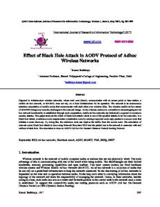
(3) . When considering omni-directional antennas and uniform propagation conditions, it is common to select Gt and Gr as 1. The use of directional antennas can permit energy savings and reduce interference by concentrating transmission energy where it is needed. We learn from [12] that because the amount of RF energy remains the same, but is distributed over less area, the apparent signal strength is higher. This apparent increase in signal strength is the antenna gain. We use an idealized model in which we assume that all of the transmitted energy is concentrated uniformly in a beam of width θ , as shown in Fig. 1, then the gain of area covered by the beam can be calculated as (1 −

2

c o s

θ 3 6 0

)

,

(4)

while the gain of the other areas is zero. As a consequence of the “wireless broadcast advantage” property of omni-directional systems [13], all nodes whose distance from Node i does not exceed rij will be able to receive the transmission with no further energy expenditure at Node i.

Fig. 1. Use of directional antenna

While using directional antenna, the advantage property will be diminished, since only the nodes located within the transmitting node’s antenna beam can receive the signal. In Fig. 1, only j, l can receive the signal, while k cannot receive the signal. We assume that the beam width θ is fixed beam width and one node can simultaneously support more than one directional antenna. Furthermore, we assume that each antenna beam can be pointed in any desired direction to provide connectivity to a subset of nodes that are within communication range. In addition, we use directional receiving antennas, which have a beneficial impact to avoid background noise and other user interferences. 2.4 Energy Expenditure In addition to RF propagation, energy is also expended for transmission (encoding, modulation, etc.) and reception (demodulation, decoding, etc.). We define

700

H. Xu et al.

• p = transmission processing power and T

• p = reception processing power. R

The total power expenditure of a node, when transmitting to a maximum range r over a sector of width θ , is p = p RF (r , θ ) + pT + p R RF

(5) R

Where p ( r , θ ) is RF propagation energy expenditure and the term p is not needed for the source node. A leaf node, since it does not transmit but only receives, has a R

total power expenditure of p .

3 Localized Directional Broadcast Incremental Power Protocol 3.1 The Proposed Algorithm The goal of the localized algorithm is to allow a localized and distributed computation of broadcast tree. We assume every node knows its local neighbors position information. The principle is as follows: the source node S (the one that initiates the broadcast) computes the broadcast tree with its local neighborhood position information and sends the broadcast packet to each of its one hop neighbor, while includes N (integer, N>0) hops computed relay information and the Nth hop relay nodes id in broadcast packet. For each of other nodes, for example, node U who receives the packet for the first time, three cases can happen: • The packet contains both relay instructions for U and U’s id. U will use these relay instructions to construct its own local broadcast tree. Then, instead of starting from an empty tree as S did, it extends the broadcasting tree based on what source S has calculated for it. By this way, the joint neighborhood nodes of S and U will use the same spanning tree. • The packet contains only relay instructions for U. U will just follow these relay instructions to relay the packet. • There are no relay instructions for U. In this case, node U does nothing. After the procedure mentioned above, node U will rebroadcast the packet again to its own one hop neighbor and include N hops computed relay information for its own relay nodes and the Nth hop relay nodes id, just like what source node has done. The reason why we use N to refer relay nodes hop number is that the range within which each node manage positional information on other nodes can be changed according to requirement, and the optimal changes according to the application demands and the node’s hardware performance. In this principle, there may be some nodes which will receive this packet more than one time, then at this time, node can simple drop the packet and doesn’t rebroadcast again. In order to reduce overlap, we use the neighbor nodes elimination scheme. Source node will include its local N hops neighbor nodes in packet, because these nodes certainly will receive the packet soon. Once the node which is in charge of

Localized Energy-Aware Broadcast Protocol for Wireless Networks

701

recalculating local spanning tree receives the packet, except recording the relay information it should also record the nodes which will be covered soon. If the covered node is not used in relay information and also is a neighbor node of this node, then this node will delete it from its neighbor list and after deletion calculate its own broadcast tree. Fig.2 is the pseudo-code of the proposed algorithm. 0. Randomly select source node S 1. For source node S: 2. { /******source node’s locale calculation******/ 3. Computes its local broadcast tree; 4. Set up broadcast packet P; 5. Include N hops relay instructions in packet P; 6. Include N hops neighbors' ID in packet P; 7. Include Nth hop relay instructions in packet P; 8. Send packet P to each of its one hop neighbor using directional antenna; 9. } 10. For any node U (except S): 11. if (node U receives packet P){ 12. if ( the first time){ 13. Inspect packet P; 14. if (there is relay instruction for U){ 15. if (U’s id exists in Nth hop relay nodes’ id){ 16. Search and record all relay instructions for U; 17. /******Neighbor Nodes Elimination Scheme******/ 18. Check included covered nodes' ID; 19. While ( (ID != U's address)&&( ID ∉ relay instruction info) ) 20. if (ID ⊂ U’s local neighbors list) 21. delete this node record from U’s local neighbors list; 22. /******U’s local calculation******/ 23. Refer recorded relay instructions; 24. Use U’s modified local neighbors list; 25. Computes U’s local broadcast tree; 26. Act as source node; 27. }else if (U’s id does not exist in Nth hop relay nodes’ id) 28. Only relay received packet as recorded relay instructions; 29. }else if (there is no relay instruction for U) 30. Do nothing; 31. } else 32. Simply drop packet P; 33. } Fig. 2. Pseudo-code of the proposed algorithm

3.2 Broadcast Tree Calculation As for how to set up broadcast tree, we have considered two basic approaches with directional antennas:

702

H. Xu et al.

• Construct the tree by using an algorithm designed for omni-directional antennas; then reduce each antenna beam to our fixed beam width. • Incorporate directional antenna properties into the tree-construction process. The first approach can be based on any tree-construction algorithm. The “beamreduction” phase is performed after the tree is constructed. The second approach which takes directional antenna into consideration at each step of the tree construction process can be used only with algorithms that construct trees by adding one node at a time. In this section, we describe the later approach applied in our algorithm LDBIP in detail. The incremental power philosophy, originally developed for use with omnidirectional antennas, can be applied to tree construction in networks with directional antennas as well. At each step of the tree-construction process, a single node is added, whereas variables involved in computing cost (and incremental cost) are not only transmitter power but beam width θ as well. In our simple system model, we use fixed beam width θ f , that means for adding a new node, we can only have two choices: set up a new directional antenna to reach a new node; raise the length range of beam to check whether there is new node covered or not. A pseudo code of the broadcast tree calculation algorithm can be written as Fig. 3. Input: given an undirected weighted graph

G(N,A), where N: set of nodes, A: set of

edges

T:={S} where S is the source node. Set P(i):= 0 for all 1 ≤ i ≤|N| where P(i) is the transmission power of node i.

Initialization: set Procedure: while |T| ≠ |N|

do find an edge (i,j)

∈ T × (N−T) with fixed beam width θ f such that ∆Pij is

minimum; if an edge (i,k) ∈ T × T raising the length range of beam can cover a node j ∈ (N−T), then incremental power ∆Pij = ∆Pij = d α θ ij

f

2π

d iαj

θ

f

2π

− P(i); otherwise,

.

add node j to T, i.e., T := T ∪ {j}. set P(i) := P(i) + ∆Pij .

Fig. 3. Pseudo code of broadcast tree calculation algorithm

Fig. 4(a) shows a simple example in which the source node has 4 local neighbor nodes 0, 1, 2, and 3. Node 1 is the closest to 0, so it is added first; in Fig. 4(b), an antenna with beam width of θ f is centered between 0 and Node 1. Then we must decide which node to add next (Node 2 or Node 3), and which node (that is already in the tree) should be its parent. In this example, the beam from 0 to Node 1 can be ex-

Localized Energy-Aware Broadcast Protocol for Wireless Networks

703

tended to include both Node 1 and Node 3, without setting up a new beam. Compared to other choices that setting up a new beam from Node 0 to Node 2, or from Node 1 to Node 2, this method has minimum incremental power. Therefore, Node 3 is added next by increasing the communication range of 0 and Node 1. In Fig. 4(c), finally, Node 1 must be added to the tree. Three possibilities are respectively to set up a new beam from 0, 1, 3. Here we assume that Node 3 has minimum distance. Then in Fig. 4 (d) we set up a new beam from Node 3 to Node 2.

(a)

(b)

(c)

(d)

Fig.4. Nodes addition in LDBI

3.3 Examples Constructed by the Various Algorithms Fig. 5 shows the broadcast tree produced by BIP, DBIP, LBIP and LDBIP for a 12node network, where the source node is shown larger than the other nodes. There broadcast trees are generated in our simulation work, which use the system model mentioned in section 2. Because DBIP and LDBIP use directional antenna, therefore in our simulation system, according to different θ f , we can get different broadcast tree; of course, the according energy consumption will also be different. Furthermore, because algorithm LBIP and our LDBIP is distributed, which means every node only calculates its two hops neighborhood broadcast tree, the Fig. 5(c) and (d) in fact is the combination of all local broadcast tree, and the joint parts of those local broadcast trees will not have too much difference because nodes refer relay information from other nodes and apply the neighbor nodes elimination scheme.

(a)

(b)

(c)

(d)

Fig. 5. Broadcast Tree. (a) BIP (b) DBIP ( θ f =30) (c) LBIP (d) LDBIP ( θ f =30)

704

H. Xu et al.

4 Performance Evaluation In this section, we present our performance evaluation for our localized algorithm LDBIP, and also compare it with two centralized algorithm BIP and DBIP which are very effective centralized protocols in energy consumption and with another localized algorithm LBIP. Especially for LBIP and LDBIP, we choose the hop number N as 2. We use ns2 as our simulation tool and assume AT&T's Wave LAN PCMCIA card as wireless node model which parameters are listed in table 1. As for system model, we apply the network, propagation, and energy model mentioned in Section 2. Table 1. Parameters for wireless node model

frequency maximum transmission range maximum transmit power receiving power transmitting power omni-antenna gain of receiver/transmitter fixed beam width of directional antennas directional antenna receiver/transmitter gain MAC protocol propagation model

AT&T's Wave LAN PCMCIA card 914MHZ 40m 8.5872e-4 W 0.395 watts 0.660 watts 1db 30 58.6955db 802.11 free space / two ray ground

The wireless network is always composed of 100 nodes randomly placed in a square area which size is changed to obtain different network density D defined as the average number of neighbors per each node. The formula can be written as: D = N *

π r2 A2 ,

(6)

where A represents the edge length of deployment square area, and r is the maximum transmission range. From Eqn. (6), we can get calculate A by A = r

Nπ D .

(7)

For each measure, 50 broadcasts are launched and for each broadcast, a new network is generated. RAR (Reach Ability Ratio) is the percentage of nodes in the network that received the message. Ideally, each broadcast can guarantee 100% RAR value. While in sparse network since the maximum transmission range of nodes is not big enough to guarantee the network connectivity, RAR may be less than 100%. To compare the different protocols, we observe the total power consumption over the network when a broadcast has occurred. We compute a ratio named EER, that represents the energy consumption of the considered protocol compared to the energy that would have been spent by a Blind Flooding (each node retransmits once with maximum transmission range). The value of EER is so defined by:

Localized Energy-Aware Broadcast Protocol for Wireless Networks

EER =

E p r o to c o l E

× 1 0 0.

705

(8)

f lo o d in g

We also observe SRB (Saved Rebroadcast) which is the percentage of nodes in the network that received the message but did not relay it. A Blind Flooding has a SRB of 0%, since each node has to retransmit once the message. Our simulation work is based on two steps: first we test the performance of our protocol in static wireless ad hoc network, and then we take mobile network into consideration. To compare the performance with those of other protocols, we observe the total power consumption over the network. In mobile simulation environment, the energy consumption includes not only the energy consumption for broadcasting message, but also that for propagation for mobility.

(a) EER comparison

(b) SRB comparison

Fig. 6. Performance comparison in static wireless network

Fig.6 shows EER and SRB comparison for BIP, DBIP, LBIP and LDBIP protocols in static wireless networks with different network density. As for the RAR value, since we choose the network density which can guarantee the network connectivity, so all the RAR results are 100%. From Fig.6 (a) we can find that all the four protocols have much better energy conservation than flooding. Because of employing directional antenna, DBIP and LDBIP have much less energy consumption compared to BIP which uses omni-directional antenna in low network density and similar saving energy performance in high network density. Also benefiting from directional antenna, compared to another localized algorithm LBIP, our proposal LDBIP has much better performance in energy conservation. In addition, the energy conservation performance of DBIP and LDBIP is stable despite of network density. Compared to centralized algorithm DBIP, our localized algorithm LDBIP has a little more energy consumption. That is because our algorithm employs the topology of only local neighbors whereas DBIP utilizes the total network topology to calculate energy efficient broadcast tree. From Fig.6 (b) we can observe localized protocols have less SRB compared to centralized protocols, since localized protocols only calculate local broadcasting tree which cause unnecessary relay instructions compared to centralized protocols. In addition, using omni-directional antenna can save more retransmission, since “wireless broadcast advantage” will be decreased by employing directional antenna.

706

H. Xu et al.

Now we take mobility into consideration. In our simulation we use mobile scenarios to simulate the nodes’ mobility in mobile networks. These mobile scenarios are randomly generated by special tool of ns2, “setdest [14]”. As we mentioned in section 2.2 positioning, in mobile network except initialization each node should set timer to check whether this node has moved or not. If mobility occurs, node will use its maximum transmission radius to emit its new location information to let other nodes update their neighborhood table. In centralized solution, this information must be propagated throughout the network, In order to compare between different protocols, we use the same mobile scenario in certain network density.

Fig. 7. EER comparison in mobile network

Fig.7 shows EER comparison for DBIP and LDBIP protocols in mobile networks with different network density. Compared to centralized algorithm DBIP in mobile network, our localized algorithm LDBIP has better energy saving performance. That is because in centralized solution, e.g. DBIP, mobility of nodes need to be broadcasted throughout the network, while in our centralized algorithm LDBIP, mobility will be only propagated to that nodes’ neighborhood. Therefore LDBIP can get better performance. From this, we can infer that as mobility increases in mobile scenarios, LDBIP can get much better performance in energy conservation. In addition, as for SRB comparison in mobile network, there is little difference with that in static network. In summary, our localized protocol LDBIP can only use localized location information and distributed computation to complete broadcasting task. Our simulation work verifies that in mobile networks, our localized energy-efficient protocol has very good performance in energy conservation.

5 Conclusions In this paper, we proposed the new localized energy-efficient broadcast protocol for wireless networks with directional antennas which have limited energy and computation resources. Our algorithm is based on the localized information and distributed computation method, which means, rather than source node collects all location information of network to calculate broadcast tree, every node collects some part of the

Localized Energy-Aware Broadcast Protocol for Wireless Networks

707

whole network’s nodes location information and participates calculating broadcast tree. At the cost of a few more information stored in the broadcast packets, our localized algorithm offers better energy saving result than well-known centralized algorithm DBIP in mobile environment. Especially, if mobility of nodes increases in network, our distributed algorithm can get lesser energy consumption and better performance than centralized solution. In future work, we plan to take realistic facts into consideration for energy consumption and network lifetime.

Acknowledgement This work was supported by grant No. R01-2005-000-10267-0 from Korea Science and Engineering Foundation in Ministry of Science and Technology.

References 1. J. E. Wieselthier, G. D. Nguyen, A. Ephremides: On the construction of energy-efficient broadcast and multicast trees in wireless networks. Proc. IEEE INFOCOM (2000) 585594 2. J.E. Wieselthier, G.D. Nguyen, A. Ephremides: Energy-Limited Wireless Networking with Directional Antennas: The Case of Session-Based Multicasting. Proc. IEEE INFOCOM (2002) 190-199 3. P. Bose, P. Morin, I. Stojmenovic, J. Urrutia: Routing with guarantee delivery in ad hoc networks. ACM/Kluwer Wireless Networks (2001) 609-616 4. T. Chu, I. Nikolaidis: Energy efficient broadcast in mobile ad hoc networks. In Proc. AdHoc Networks and Wireless (ADHOC-NOW), Toronto, Canada (2002) 177-190 5. W. Peng, X. Lu: On the reduction of broadcast redundancy in mobile ad hoc networks. In Proc. Annual Workshop on Mobile and Ad Hoc Networking and Computing (MobiHoc'2000), Boston, Massachusetts, USA (2000) 129-130 6. A. Qayyum, L. Viennot, A.Laouiti: Multipoint relaying for flooding broadcast messages in mobile wireless networks. In Proc. 35th Annual Hawaii International Conference on System Sciences (HICSS-35), Hawaii, USA (2002) 7. J. Wu, H. Li: A dominating-set-based routing scheme in ad hoc wireless networks. In Proc. 3rd Int'l Workshop Discrete Algorithms and Methods for Mobile Computing and Comm (DIALM'99), Seattle, USA (1999) 7-14 8. F.Ingelrest, D.Simplot-Ryl: Localized Broadcast Incremental Power Protocol for Wireless Ad Hoc Networks. 10th IEEE Symposium on Computers and Communications (ISCC 2005), Cartagena, Spain (2005) 9. E.D. Kaplan: Understanding GPS: Principles and Applications. Artech House (1996) 10. H.T. Friis: A note on a simple transmission formula. Proc. of the IRE, Vol. 41, May (1946) 254-256 11. H.T. Friis: Introduction to radio and radio antennas. IEEE Spectrum, April (1971) 55-61 12. Joseph J. Carr: Directional or Omni-directional Antenna. Joe Carr's Receiving Antenna Handbook, Hightext (1993) 13. J.E. Wieselthier, G.D. Nguyen, A. Ephremides: Algorithms for Energy-Efficient Multicasting in Static Ad Hoc Wireless Networks. Mobile Networks and Applications (MONET), vol. 6, no. 3 (2001) 251-263 14. Network Simulator - ns-2, http://www.isi.edu/nsnam/ns/.