1
Locality-Based Aggregate Computation in Wireless Sensor Networks Jen-Yeu Chen, Member, IEEE, Gopal Pandurangan, Member, IEEE, and Jianghai Hu, Member, IEEE
Abstract The design of efficient gossip-based protocols for computing aggregate functions in wireless sensor network has received considerable attention recently. A primary reason for this surge in interest is their robustness due to their randomized nature. In addition, because of the inherent simplicity in their design, gossip-based protocols are suitable to be implemented on sensor nodes with limited computing capability and battery power. In the context of energy-constrained sensor networks, it is of paramount importance to reduce the message and time complexity of gossip-based protocols. In this paper, we present DRRgossip, an energy-efficient and robust aggregate computation algorithm in sensor networks. Exploiting locality, the Distributed Random Ranking (DRR) algorithm first builds a forest of disjoint local trees over the sensor network. The height of each tree is small, so that the aggregates of the tree nodes can be quickly obtained at the root of the tree. All the roots then perform a uniform gossip algorithm on their respective aggregates to reach a distributed consensus on the global aggregate. We prove that the 3/2
DRR-gossip algorithm requires O(n) messages and O( logn1/2 n ) transmissions to obtain aggregates on a random geometric graph. This reduces the energy consumption by at least a factor of
1 log n
over the
standard uniform gossip algorithm. Experiments validate the theoretical results and show that DRR-gossip needs much less transmissions than other gossip-based schemes. Index Terms wireless sensor networks; aggregate computation; gossip; distributed algorithm; randomized algorithm; random geometric graph
Jen-Yeu Chen is with the Department of Electrical Engineering, National Dong Hwa University, Taiwan, R.O.C. Email:
[email protected]. Gopal Pandurangan is with the Department of Computer Science, Purdue University, West Lafayette, USA. E-mail:
[email protected]. Jianghai Hu is with the School of Electrical and Computer Engineering, Purdue University, West Lafayette, USA. E-mail:
[email protected].
2
I. I NTRODUCTION Aggregate statistics such as Average, Max/Min, Sum and Count have been significantly useful for many applications in sensor networks [2], [4], [9], [10], [14], [21]. Many research efforts have been dedicated to developing scalable and distributed algorithms for the computation of aggregates in sensor networks. Among them gossip-based algorithms [1], [2], [3], [8], [9], [12], [15], [18], [20] have recently received much attention because of their simplicity for implementation, scalability to large network size, and robustness to frequent network topology changes. In a standard gossip algorithm, every node computes and updates the approximate of the target aggregate iteratively. In an iteration, every node randomly selects another node to transmit the information of its current approximate. As a result, each node’s approximate will gradually approach the correct aggregate. In the end, all the approximates will reach a consensus, within some accuracy threshold, on the target aggregate. There may be substantial energy waste in a standard gossip algorithm. It has been shown in [1] that the neighboring gossip algorithm1 , where a node randomly selects a neighboring node to exchange information, needs the same order of radio transmissions, O(n2 ), as the plain flooding on a Poisson random geometric graph. In [9] another version of gossip, named uniform gossip, allows that every node uniformly at random selects another node in the network to send its data. Multi-hop routing is necessary for uniform gossip. To reach the global consensus on aggregate, the uniform gossip needs O(log n) rounds, O(n log n) messages and O(D · n log n) transmissions in the worst case, where D is
the diameter of the network. Recently, some novel gossip-based algorithms have been proposed to improve the performance of a standard gossip algorithm. The geographic gossip of [3] adopts the neighboring gossip scheme but allows two remote nodes to exchange information by geographic routing, improving the cost of transmissions to O(n3/2 log3/2 n) from the neighboring gossip’s O(n2 ). The efficient gossip in [8], an improvement of uniform gossip scheme where groups are formed before applying uniform gossip, needs a slightly longer time O(log n log log n), but reduces the messages and transmissions to O(n log log n) and O(D · n log n), respectively. A different approach, the hierarchical spacial gossip [20],
using ODI-synopsis and restricting the communications locally, needs a longer O(poly(log n)) time but requires only O(n poly(log n)) transmissions. In this paper, a novel approach named the DRR-gossip algorithm is presented. Exploiting locality, a Distributed Random Ranking algorithm, DRR, is used to first build a forest of (disjoint) localized trees 1
The neighboring gossip is called the fastest gossip in [1] as its diffusion speed can be optimized by carefully setting the
selection probability.
3
over the sensor network. The height of a tree is small, thus the aggregates of its nodes can be quickly obtained at its root. All the roots then perform the uniform gossip algorithm on their respective aggregates to reach distributed consensus on the global aggregate. Compared with the standard uniform gossip, 3/2
our DRR-gossip algorithm requires O(n) messages and O( logn1/2 n ) transmissions to reach consensus, reducing the energy consumption by at least a factor of 1/ log n on a Poisson random geometric graph. The DRR-gossip algorithm is inspired from the efficient gossip ([8]) idea of reducing the number of nodes participating in the gossip process in order to decrease the numbers of messages and transmissions for achieving consensus. Further, our DRR-gossip algorithm takes advantage of the locality of the trees to further decrease the number of messages to O(n) while still maintains a running time of O(log n), whereas the efficient gossip algorithm needs O(log n log log n) time and O(n log log n) messages. The DRR-gossip algorithm proceeds in phases. In phase one, all the sensor nodes run the DRR algorithm to construct a forest of disjoint ranking trees. In phase two, within each ranking tree, the local aggregate (e.g. sum or maximum) of a ranking tree is computed by a convergecast process and obtained at the root of the tree. In phase three, all the roots of the ranking trees utilize a suitably modified version of the uniform gossip algorithm [9] to obtain the global aggregate. Finally, if necessary, a root can forward the global aggregate along the tree branches to all the other nodes of the tree. The rest of this paper is organized as follows. The network model is described in Section II followed by sections where each phase of the DRR-gossip algorithm is introduced and analyzed separately. The whole DRR-gossip algorithm is summarized in Section VI. Simulation results are provided in Section VII. We finally conclude in Section VIII. II. N ETWORK MODEL A wireless sensor network is abstracted as a connected undirected graph G(V, E) with all the sensor nodes as the set of vertices V and all the bi-directional wireless communication links as the set of edges E . This underlying graph can be arbitrary depending on the deployment of sensor nodes. Let each sensor
node i be associated with an initial observation or measurement value denoted as vi ∈ R. The assigned values over all vertices form a vector v. The goal is to compute aggregate functions such as average, sum, max, min etc. on the vector of values v. For ease of understanding, we present and analyze the DRR-gossip algorithm in synchronized rounds, even though the algorithm is not required to be synchronized. All the sub-procedures work in asynchronous setting though the analysis is more involved and needs to be altered. The DRR-gossip algorithm is an application layer algorithm to which the underlying layers should be
4
transparent. Thus, we do not assume any particular MAC and PHY layers for message transmissions but assume that all the nodes of the undirected connected graph G can simultaneously send a message to their one-hop neighbors in a “step” of the algorithm2 . In phase one and phase two of the DRR-gossip algorithm, all messages require only local one-hop transmissions whereas in phase three messages may require multi-hop transmissions. The time for a gossip message to reach its destination is a “round” of the gossip algorithm. Thus, in the phase three, the gossip algorithm proceeds in rounds, each of which contains several steps. The length of a message is limited to O(log n + log s), where s is the range of measured values on sensor nodes.
III. P HASE I: D ISTRIBUTED R ANDOM R ANKING A. The DRR algorithm The DRR algorithm is implemented in the following way. On an undirected connected graph G = (V, E), every node i ∈ V uniformly at random generates a random value, rank(i) ∈ [0, 1], named the
rank3 of node i, and then sends its rank to all its (one-hop) neighboring nodes. Each node compares the ranks it receives with its own and then connects to the node of the highest rank among all of its neighbors and itself. If a tie between two ranks happens, nodes can break the tie by their identifiers. Through these connections, many disjoint “local ranking trees” are established on the graph. These trees together constitute a forest F, which is a subgraph of G , i.e., F(V 0 , E 0 ) ⊆ G(V, E), where V 0 = V and E 0 ⊆ E . If a node is of the highest rank among its neighbors and itself, it becomes the root of a tree.
Since every node, except the root nodes, connects to a node with a higher rank, there is no loop in the constructed graph, the forest F. The pseudo-code of the DRR algorithm is provided in Algorithm 1. An example to illustrate the result of the DRR algorithm is shown in Fig. 1. The Poisson random geometric graph shown in Fig. 1(a) has 400 nodes in a unit square. After running the DRR algorithm, the constructed forest of ranking trees is shown in Fig. 1(b). In this paper we focus our analysis on Poisson random geometric graphs, a useful and popular graph model for sensor networks [5], [17], though the analysis can be extended to general graphs. A Poisson
2
In wireless MAC layer, two neighboring nodes can not send messages simultaneously. One node needs to send its message
after the other one finishes. In application layer, we define the necessary time period for nodes to successfully finish their transmissions as one “step” of the algorithm. Obviously, the time period of a step will vary according to the underlying MAC layer. 3
The rank of a node i, rank(i), is independent of its value vi .
5
Algorithm 1: F =DRR(G) 1
foreach node i ∈ V do
2
independently and uniformly at random generate a rank rank(i) ∈ [0, 1];
3
send rank(i) to all its neighboring nodes j ∈ N(i) where N(i) = {j|(i, j) ∈ E};
4
collect the ranks from its neighbors and compare them with its own rank. Let ψ = maxj∈N(i) rank(j);
5
if ψ > rank(i) then set parent(i) = argmaxj∈N(i) rank(j);
6 7
else set parent(i) = NULL, and become a root node.
8 9
end
10
send a connection message including its identifier, i, to its parent node parent(i);
11
collect the connection messages and accordingly construct the set of its children nodes, Child(i);
12
if Child(i) = ∅ then become a leaf node;
13 14
else become an intermediate node.
15 16 17
end end
random geometric graph is denoted by G(n, r(n)) = G(V, E), where |V | = n and the radius r(n) = Ω(( logn n )1/2 ) to maintain connectivity [5].
B. The expected number of ranking trees and the locality of a ranking tree To find the expected number of ranking trees, i.e., the expected number of roots, generated by the DRR algorithm on a Poisson random geometric graph, we need the following lemma. Lemma 1: At the end of the DRR algorithm, a node i ∈ V of degree di in graph G becomes the root of a local ranking tree with the probability 1/(di + 1). Due to space limitation, we refer to appendix for the proof. The following theorem shows the expected number of roots in a Poisson random geometric graph.
6
Theorem 2: On a Poisson random geometric graph G(n, r), the expected number of ranking trees constructed by the DRR algorithm is m = O( logn n ). Proof: Given a Poisson random geometric graph G(n, r), an n-tuple random variable d~ = (d1 , d2 , . . . , dn ), where di is the degree of node i ∈ V , is used to represent the degrees of all nodes of a possible instance of the random geometric graph G. The degree di is a random variable determined by the 2-D homogeneous Poisson point process with intensity n. Let Yi be the indicator for the event that the node i ∈ V becomes a root and Y =
P i∈V
Yi be the
random variable indicating the total number of roots after running the DRR algorithm. Given d~, the expected number of roots is then E[Y | d~ ] =
X
E[Yi | d~ ] =
i∈V
So, letting γ = (
Pn
k=0 e
X i∈V
1 . di + 1
k
−λ λ )−1 k!
= Θ(1), the expected number of roots of the local ranking trees is h i X · 1 ¸ ~ E[Y ] = E E[Y | d ] = E di + 1 i∈V
= γn ·
n X k=0
1 λk · e−λ k+1 k! n
γn −λ X λk+1 ·e λ (k + 1)! k=0 µ µ n+2 ¶¶ γn −λ λ λ = ·e e −1−o λ (n + 2)! µ µ µ n+2 ¶¶¶ γn λ = 1 − e−λ 1 + o , λ (n + 2)! =
where λ = n · πr2 = Ω(log n) is the expected degree of a node in the Poisson random geometric graph. In the above, the third equality follows from the fact that every node has the same degree distribution determined by a 2-D Poisson point process. Thus, running Distributed Random Ranking on a Poisson random geometric graph with the number of nodes n, the expected number of roots E[Y ] is O( logn n ), ¢ γn ¡ 1 n i.e., E[Y ] ≤ log n 1 − n = O( log n ). Locality of a ranking tree To show the locality of a ranking tree, we need to bound the maximal height of a local ranking tree in the Poisson random geometric graph G(n, r). To do this, some definitions and lemmas are needed. Definition 3: An h-hop path {i1 , i2 , . . . , ih+1 } in graph G(V, E) is an ordered sequence of h + 1 nodes where each node is only encountered once (i.e., the multitude of any node in a path equals to one)
7
and any two consecutive nodes are adjacent to each other, i.e., (ik , ik+1 ) ∈ E , for 1 ≤ k ≤ h. Definition 4: An h-hop potential ranking path {i1 , i2 , . . . , ih+1 } in a graph G(V, E) is an h-hop path where each node is only adjacent, in the graph G, to its preceding node and its following node, i.e., (ik , ik+1 ) ∈ E , for 1 ≤ k ≤ h and (ik , ik+s ) ∈ / E , for 1 ≤ k ≤ h − 1 and 1 < s ≤ h + 1 − k .
Definition 5: A rooted tree path is a simple path contained entirely within a ranking tree, with the starting node the root of the ranking tree. Lemma 6: Any rooted tree path is a potential ranking path. Due to space limitation, we refer to appendix for the proof. Note that a potential ranking path is not necessarily a rooted tree path whereas a rooted tree path has to be a potential ranking path. Lemma 7: Given a path of length h in a Poisson random geometric graph, the probability that it is a potential ranking path of length h is O(( 23 )h−1 ). Due to space limitation, we refer to appendix for the proof. Theorem 8 (Locality of ranking trees): On a Poisson random geometric graph G(n, r),w.h.p.4 , the height of the ranking trees constructed by the DRR algorithm is bounded by O(log n). Proof: We show that the probability that an h-hop path, starting from a root, is a rooted tree path is asymptotically close to zero when h = Θ(log n). First, this path is a potential ranking path with probability O((2/3)h−1 ). Secondly, conditioning on that it is a potential ranking path, this h-hop potential ranking
path is an h-hop rooted tree path only if all the nodes’ ranks on this path are in a strictly decreasing order, which happens with probability 1/(h + 1)!. Let h + 1 = Θ(log n). The probability that an h-hop path, starting from a root, is a rooted tree path is at most
1 (h+1)!
· O(( 32 )h−1 ) = o(( 23 )2h ) = o(( 32 )2 log n ) =
o(n−α ); α > 0.
We further show that the expected number of (log n)-hop rooted tree paths, Z , is asymptotically close to zero. On a Poisson random geometric graph, the total number of h-hop paths starting from a root is O(logh n), w.h.p., since the degree of a node is bounded by O(log n) w.h.p., [5]. Letting h = c · log n
4
The term with high probability, w.h.p., means with probability at least 1 − O(n−α ) for some positive constant α.
8
and using Stirling’s approximation, Ã Z=O
1 · (h + 1)!
! µ ¶h−1 2 · logh n 3
µ
¶ (log n)c log n (2/3)c log n =O (2πc log n)1/2 (c log n/e)c log n µ ¶ µ ¶ (2e/3c)c log n n−α =O =O , (2πc log n)1/2 (2πc log n)1/2
where α = c(log( 3c 2 ) − 1). By suitably fixing c, we have α > 1 and that Z is asymptotically close to zero. Hence the probability that a tree is of height O(log n), i.e., the probability that there exists a rooted tree path of length O(log n) is asymptotically close to zero. Therefore, w. h. p. the height of a local ranking tree is bounded by O(log n). C. Advantages of the DRR algorithm The DRR algorithm has the following advantages: (1) locality; (2) robustness to adversary; and (3) easy load balancing. First, from the above Theorem 8, a message originating from a leaf of a local ranking tree needs at most O(log n) relays to arrive at the root of the tree. Local aggregates of a ranking tree can be quickly obtained at the root node with low cost of messages and transmissions. Secondly, consider a deterministic approach that constructs local trees rooted at some pre-determined roots. An adversary can easily locate a root node and destroy it since the root’s location is fixed. In contrast, the DRR algorithm has the robustness against the adversary since the roots are randomly distributed in the network. Also, running the DRR algorithm periodically to change roots can balance the transmission load over nodes in the network. D. Complexity of the DRR algorithm In step 2 of the algorithm, every node needs to broadcast its rank to its neighbors. This costs O(|V | = n) messages in a round since every node uses wireless transmission. In step 4, all the nodes except the roots of local ranking trees have to send a message to their parent nodes, requiring totally O(|V | = n) messages in a round. Totally in these two steps, the message complexity is O(n). By Theorem 8 the time complexity is O(log n). IV. P HASE II: C ONVERGE - CAST In the second phase of our algorithm, the local aggregate of each tree will be obtained at the root by the Convergecast algorithm — an aggregation process starting from the leaf nodes and proceeding upward
9
Algorithm 2: convmax =Converge-cast-max(F,v) Input: the ranking forest F, and the value vector v over all nodes in F Output: the local M ax aggregate vector convmax over roots 1
foreach leaf node do send its value to its parent;
2
foreach intermediate node do
3
- collect values from its children;
4
- compare collected values with its own value;
5
- update its value to the maximum amid all and send the maximum to its parent.
6
end
7
foreach root node z do
8
- collect values from its children;
9
- compare collected values with its own value;
10 11
- update its value to the local maximum value convmax (z). end
along the tree to the root node. For example, to compute the local max/min, all leaf nodes simply send their values to their parent nodes. An intermediate node collects the values from its children, compares them with its own value and sends its parent node the max/min value among all received values and its own. A root node then can obtain the local max/min value of its tree. The pseudo-code of the Convergecast-max algorithm and the Converge-cast-sum algorithm are provided in Algorithm 2 and Algorithm 3, respectively. In the pseudo-codes, the input v ∈ Mn,1 , where Mx,y is the x × y matrix, represents the value vector over all nodes in V ; the output convmax ∈ Mm,1 and convsum ∈ Mm,2 are the computed aggregates at root nodes, where m is the number of root nodes. A. Complexity of Converge-cast Every node except the root nodes needs to send a message to its parent in the upward aggregation process of the Converge-cast algorithms. So the message complexity and transmission complexity are both O(n). It directly follows from Theorem 8 that the time complexity is O(log n). V. P HASE III: G OSSIP ON THE OVERLAY COMPLETE GRAPH In the third phase, all roots of the local ranking trees compute the global aggregate by performing ˜ = clique(V˜ ), where V˜ ⊆ V is the set the uniform gossip algorithm on an abstract overlaying graph G
10
Algorithm 3: convsum =Converge-cast-sum(F,v) Input: the ranking forest F and the value vector v over all nodes in F Output: the local Ave aggregate vector convmax over roots. 1
Initialization: every node i stores a row vector (vi , wi = 1) including its value vi and a size count wi
2
foreach leaf node i ∈ F do
3
- send its parent a message containing the vector (vi , wi = 1)
4
- reset (vi , wi ) = (0, 0).
5
end
6
foreach intermediate node j ∈ F do
7 8
- collect messages (vectors) from its children P P - compute and update vj = vj + k∈Child(j) vk , and wj = wj + k∈Child(j) wk , where Child(j) = {j ’s children nodes}
9 10
- send computed (vj , wj ) to its parent - reset its vector (vj , wj ) = (0, 0) when its parent successfully receives its message.
11
end
12
foreach root node z do
13 14
- collect messages (vectors) from its children P - compute the local sum aggregate convsum (z, 1) = vz + k∈Child(z) vk , and the size count of P the local ranking tree convsum (z, 2) = wz + k∈Child(z) wk , where Child(z) = {z ’s children nodes}.
15
end
˜ , a message may need a multi-hop relay, i.e., of roots and |V˜ | = m. To traverse through an edge of G
several one-hop transmissions, on the original physical network graph G. Exploiting the abundant research results on routing algorithms on sensor networks (e.g., [23], [22], [11]), roots can communicate with each other by using one of these routing algorithms. In particular, the (greedy) geographic routing [6], [3], [19], [13] by which a source node can route its message to the node closest to a chosen position (coordinate) without knowing the identifier of the destination node is suitable for the roots to perform uniform gossip since a root node does not know where and who the other roots are. We will discuss this in more detail in Section VI-B1.
11
The idea of uniform gossip is as follows. Every root independently and uniform at random selects a node to send (or say, gossip) its message. If the selected node is another root then the task is completed. If not, then the selected node needs to forward the received message to its root by multi-hop relaying upward its ranking tree. Thus, in a sense, each ranking tree becomes a super node and all the super nodes ˜. form a complete graph, G
The algorithm 4, Gossip-max, and the algorithm 6, Gossip-ave (a modification of the Push-Sum algorithm of [9], [8]) , compute the M ax and Ave aggregates respectively. Note that there is no sampling procedure in the Gossip-ave algorithm. The algorithm 5, Data-spread, is a modification of the Gossip-max algorithm for a root node to spread its value. If a root needs to spread a particular value over the network, it sets that particular value as its initial value of the Gossip-max algorithm and all the other roots set their initial values to minus infinity. A. Performance of the Gossip-max and Data-spread algorithms Let m, n denote the number of the root nodes and the number of all the nodes of a sensor network, respectively. We have m = |V˜ | = O(n/ log n) and n = |V |. Karp et al. [7] gave a rumor spreading algorithm (for spreading a data item, such as M ax, throughout a network of n nodes) that takes O(log n) communication rounds and O(n log log n) messages. Their Push algorithm, a prototype of our Gossipmax algorithm, uses uniform selection probability, i.e., each node is chosen with equal probability. Similar to the Push algorithm, the Gossip-max algorithm needs O(m log m) = O(n) messages for all the roots to obtain M ax if the selection probability is uniformly 1/m. However, in the implementation of the Gossip-max algorithm on the ranking tree forest, the root of a ranking tree is selected with a probability proportional to the size of its associated ranking tree. The uniformity of the selection probability does not hold here even though the fluctuation of the tree size may be small. In this case, we can only guarantee that after the gossip procedure of the Gossip-max algorithm, a portion of the roots including the root of the largest tree will possess the M ax. After the gossip procedure, roots can sample an O(log n) number of other roots to confirm and update, if necessary, their values to reach the consensus on M ax. To analyze the performance of the Gossip-max algorithm, we assume that a message may fail to reach the selected root node with probability ρ while it travels through the network. The message may fail at the routing stage or at the forwarding stage along the ranking tree toward the root node. But the probability to fail at the latter stage is typically much smaller than at the former one as the height of a local ranking tree is relatively much smaller than the average hop-count of a routing path. We set ρ = 1 − (1 − ρ1 )(1 − ρ2 ) ≈ ρ1 , where ρ1 , ρ2 are the failure probabilities at the above two stages
12
Algorithm 4: x ˆmax =Gossip-max(G, F, V˜ , convmax ) Initialization: every root i ∈ V˜ is of the maximum value x0,i = convmax (i) computed from the
1
Converge-cast-max algorithm. 2
gossip procedure:
3
for t=1 : O(log n) rounds do Every root i ∈ V˜ independently and uniformly at random selects a node in V and sends the
4
selected node a message containing its current value xt−1,i . 5
Every node j ∈ V − V˜ forwards any received messages along its ranking tree to its root.
6
Every root i ∈ V˜
7
- collects messages and compares the received values with its own value
8
- updates its current value xt,i , node i’s current estimate of M ax, to the maximum amid all received values and its own. end
9 10
sampling procedure:
11
for t=1 :
1 c
log n rounds do
Every root i ∈ V˜ independently and uniformly at random selects a node in V and sends each of
12
the selected nodes an inquiry message. 13
Every node j ∈ V − V˜ forwards any received inquiry messages to its root.
14
Every root i ∈ V˜ , upon receiving inquiry messages, sends the inquiring roots its value.
15
ˆ max,t (i), to the maximum value it inquires. Every root i ∈ V˜ , updates xt,i , i.e. x
16
end
ˆ ru =Data-spread(G, F, V˜ , xru ) Algorithm 5: x 1
Initialization: A root node i ∈ V˜ who intends to spread its value xru , |xru | < ∞ sets up x0,i = xru . All the other nodes j set up x0,j = −∞.
2
Run gossip-max(G, F, V˜ , x0 ) by the initialized values.
respectively. For convenience, we call those roots which have already known the M ax as max-roots and those which have not as the non-max-roots. 1) Gossip procedure:
13
Algorithm 6: x ˆave =Gossip-ave(G, F, V˜ , convsum ) 1
Initialization: Every root i ∈ V˜ sets up a vector (s0,i , g0,i ) = convsum (i), where s0,i and g0,i are the local sum of values and the size of the local ranking tree rooted at i, respectively.
2 3
for t = 1 : O(log m + log(1/²)) rounds do Every root node i ∈ V˜ independently and uniformly at random selects a node in V and sends the selected node a message containing a row vector (st−1,i /2, gt−1,i /2).
4
Every node j ∈ V − V˜ forwards any received messages to the root of its ranking tree.
5
Let At,i ⊆ V˜ be the set of roots whose messages reach root node i at round t. Every root node
6 7
i ∈ V˜ updates its row vector by P st,i = st−1,i /2 + j∈At,i st−1,j /2, P gt,i = gt−1,i /2 + j∈At,i gt−1,j /2.
8
Every root node i ∈ V˜ updates its estimate of the global average by ˆ ave,t (i) = x x ˆave,t,i = st,i /gt,i .
9
end
˜ = clique(V˜ ) of G(V, E) will result in, w.h.p., Theorem 9: Running the Gossip-max algorithm on G c·n at least Ω( log n ) root nodes having the global maximum, M ax, where n = |V | and 0 < c < 1 is a
constant. Proof: Let Rt be the number of max-roots in round t. Our proof is in two steps. We first show that, w.h.p., Rt > 4 log n after 8 log n/(1 − ρ) rounds of Gossip-max. If R0 > 4 log n then the task is completed. Consider the case when R0 < 4 log n. Since the initial number of max-roots is small in this case, the chance that a max-root selects another max-root is small. Similarly, the chance that two or more max-roots select the same root is also small. So, in this step, w.h.p. a max-root will select a non-max-root to send out its gossip message. If the gossip message successfully reaches the selected non-max-root, Rt will increase by 1. Let Xi denote the indicator of the event that a gossip message i from some max-root successfully reaches the selected non-max-root. We have P r(Xi = 1) = (1 − ρ). P8 log n/(1−ρ) Then X = i=1 Xi is the minimal number of max-roots after 8 log n/(1 − ρ) rounds. Clearly, E[X] = 8 log n. Here we conservatively assume the worst situation that initially there is only one max-
root and at each round only one max-root selects a non-max-root. So X is the minimal number of max-roots after 8 log n/(1 − ρ) rounds. For clarity, let n ˜ = 8 log n/(1 − ρ). Define a Doob martingale sequence Z0 , Z1 , . . . , Zn˜ by setting Z0 = E[X], and, for 1 ≤ i ≤ n ˜ , Zi = E[X|X1 , . . . , Xi ]. It is clear
14
that Zn˜ = X and, for 1 ≤ i ≤ n ˜ , |Zi − Zi−1 | ≤ 1. Applying Azuma’s inequality and setting ² = 1/2: P r(|X − E[X]| ≥ ²E[X]) = P r(|Zn˜ − Z0 | ≥ ²E[X]) Ã ! Ã ! ²2 E[X]2 ²2 E[X]2 ≤ 2 exp − Pn˜ = 2 exp − 8 log n 2 i=1 12 2( 1−ρ ) ³ ´ = 2 exp log n−(1−ρ) = 2 · n−(1−ρ) ,
where ρ could be arbitrarily small. Without loss of generality, let ρ < 1/4. Then P r(|X − E[X]| ≥ 3
²E[X]) ≤ 2·n− 4 . Hence, w.h.p., after 8 log n/(1−ρ) = O(log n) rounds, Rt ≥ R0 +X > R0 + 12 E[X] = R0 + 4 log n > 4 log n.
In the second step of our proof, we find the lower bound of the increasing rate of Rt when Rt > 4 log n. In each round, there are Rt messages sent out from max-roots. Let Yi denote the indicator of an event that a message i from a max-root successfully reaches a non-max-root. Yi = 0 when either of the following events happen: (1) The message i fails in routing to its destination; (2) The message i is sent to another max-root, even though it successfully travels over the network. The probability of this event is at most (1−ρ)Rt log n n
since w.h.p. the size of a ranking tree is O(log n). (3) The message i and at least another
message are destined to the same non-max-root. As the probability of three or more messages destining to the same node is much smaller, we only consider the case that two messages select the same nonmax-root. We conservatively exclude both two messages on their possible contributions to the increase of Rt . This event happens with a probability at most
(1−ρ)Rt log n . n
Applying the union bound [16], P r(Yi = 0) ≤ ρ +
Since Rt ≤
cn log n
2(1 − ρ)Rt log n . n
for any constant 0 < c < 1/2 (otherwise, the task is completed), P r(Yi = 0) ≤ ρ + 2c(1 − ρ) = c0 + (1 − c0 )ρ,
where c0 = 2c < 1 is a constant that is suitably fixed so that c0 + (1 − c0 )ρ < 1. Consequently, we P t 0 have P r(Yi = 1) > (1 − c0 )(1 − ρ), and E[Y ] = R i=1 E[Yi ] > (1 − c )(1 − ρ)Rt . Applying Azuma’s inequality, µ 2 ¶ ² E[Y ]2 P r(|Y − E[Y ]| > ²E[Y ]) < 2 exp − 2Rt ¶ µ 2 0 2 ² (1 − c ) (1 − ρ)2 Rt . < 2 exp − 2
15
Since in this step, w.h.p., Rt > 4 log n, and (1 − c0 )2 (1 − ρ)2 > 0, setting ² =
1 2
and α = O(1), we
obtain 1 P r(Y < (1 − c0 )(1 − ρ)Rt ) < 2 · n−α . 2
Thus, w.h.p., Rt+1 > Rt + 12 (1 − c0 )(1 − ρ)Rt = βRt , where β = 1 + 12 (1 − c0 )(1 − ρ) > 1. Therefore, c·n w.h.p., after (8 log n/(1 − ρ) + logβ n) = O(log n) rounds, at least Ω( log n ) roots will have the M ax. cn 2) Sampling procedure: From Theorem 9, after the gossip procedure, there are Ω( log n ) = Ω(cm),
0 < c < 1, nodes with the M ax. For all the roots to reach the consensus on M ax, all the roots then
sample each other as in the sampling procedure. It is possible that the root of a larger ranking tree will be sampled more frequently than the roots of smaller trees. However, this non-uniformity is an advantage, since the roots of the larger ranking trees could have obtained the M ax in the gossip procedure with a higher probability due to this same non-uniformity. In the sampling procedure, a root without M ax can obtain M ax with higher probability through this non-uniform sampling. ˜ = clique(V˜ ) of Theorem 10: Running the Gossip-max algorithm on the overlay complete graph G G(V, E), after the sampling procedure, w.h.p., all the roots will know the M ax.
Proof: After the sampling procedure, the probability that none of the max-roots is sampled by a ¡ ¢ 1 log n c non-max-root is at most m−cm < n1 . Thus, after the sampling procedure, any root node will know m the M ax with probability at least 1 − n1 . 3) Complexity of the Gossip-max and the Data-spread algorithms: The gossip procedure takes O(log n) rounds and O(m log n)=O( logn n log n)=O(n) messages. The sampling procedure takes O( 1c log n)=O(log n) rounds and O( m c log n)=O(n) messages. To sum up, the Gossip-max algorithm in total takes O(log n) rounds and O(n) messages for all the roots in a network to reach consensus on M ax w.h.p. The complexity of the Data-spread algorithm is the same as the Gossip-max algorithm. B. Performance of the Gossip-ave algorithm In the case that the uniformity of gossip is held, it has been shown in [9] that on an m-clique with probability at least 1 − δ 0 , Gossip-ave (uniform push-sum in [9]) needs O(log m + log 1² + log δ10 ) rounds and O(m(log m + log 1² + log δ10 )) messages for all the m nodes to reach consensus on the global average with a relative error at most ². When the uniformity does not hold, the performance of uniform gossip will depend on the distribution of the selection probability. It has been shown in [8] that by using the efficient gossip algorithm the node being selected with the largest probability will have the global average, Ave, in O(log m + log 1² ) rounds. In the following, we prove that the same upper bound holds for our
16
Gossip-ave algorithm, namely, the root of the largest tree will have Ave after O(log m + log 1² ) rounds of the gossip procedure. We need some definitions as in [9]. We define an m-tuple contribution vector yt,i such that st,i = yt,i · x =
X
yt,i,j xj
j
and wt,i = kyt,i k1 =
X
yt,i,j ,
j
where yt,i,j is the j -th entry of yt,i and xj is the initial value at root node j , i.e., xj = convsum (j), the local aggregate of the ranking tree rooted at node j computed by Converge-cast-sum. y0,i = ei , the P P unit vector with the i-th entry being 1. Therefore, i yt,i,j = 1, and i wt,i = m. When yt,i is close to
1 m 1,
where 1 is the vector with all entries 1, the approximate of Ave, x ˆave,t,i =
st,i gt,i ,
is close to the
true average xave . Note that wt,i which is different from gt,i is a dummy parameter borrowed from [9] to characterize the diffusion speed. In our Gossip-ave algorithm, we set g0,i to be the size of the root i’s ranking tree. The algorithm then computes the estimate of average directly by x ˆave,t,i = st,i /gt,i .
If we set a dummy weight wt,i , whose initial value w0,i = 1, ∀i ∈ V˜ , the algorithm performs in the same manner as that every node works on a triplet (st,i , gt,i , wt,i ) and computes x ˆave,t,i =
(st,i /wt,i ) , (gt,i /wt,i )
where (st,i /wt,i ) is the estimate of the average local sum on a root and gt,i /wt,i is the estimate of the average size of a ranking tree. Their relative errors are bounded in the same way as follows. The relative error in the contributions (with respect to the diffusion effect of gossip) at node i at time yt,i,j t is ∆t,i = maxj | ky − t,i k1
1 m|
yt,i,j = k ky − t,i k1
1 m k∞ .
Also, a potential function Φt =
X i,j
(yt,i,j −
wt,i 2 ) m
is the sum of the variance of the contributions yt,i,j . We name the root of the largest ranking tree as z . For the upper bound of the running time of the Gossip-ave algorithm, we have the following theorem. Theorem 11: W.h.p., there exists a time Tave = O(log m + α log n) = O(log n), α > 0, such that for all time t ≥ Tave , the relative error of the estimate of average aggregate on the root of the largest ranking
17
tree, z , is at most
2 nα −1 ,
where the relative error is
|ˆ xave,t,z −xave | |xave |
and the global Ave is xave =
P j
xj ,
when all xj have the same sign. To prove this theorem we need some auxiliary lemmas. Due to the space limitation, we refer to appendix for their proofs. Lemma 12 (geometric convergence of Φ): The conditional expectation E[Φt+1 |Φt = φ] = 12 (1 − P gi 1 2 i∈V˜ Pi )φ < 2 φ, where Pi = (1 − δ) n is the probability that the root node i is selected by other root nodes; gi is the size of ranking tree rooted at node i; δ is the probability that a message fails to reach its destined root node and n is the total number of nodes in the network. Lemma 13: There exists a τ = O(log m) such that after ∀t > τ rounds of Gossip-ave, wt,z ≥ 2−τ at the root z of the largest ranking tree. From the previous two lemmas, we derive the following theorem. Theorem 14 (diffusion speed of Gossip-ave): With probability at least 1−δ 0 ,there exists a time Tave = O(log m + log 1² + log δ10 ), such that ∀t ≥ Tave , the contributions at the root, z , of the largest ranking yt,z,y tree is nearly uniform, i.e., k ky − t,z k1
1 m k∞
≤ ², where δ 0 > 0 and ² > 0 are constants.
Proof: By Lemma 12, we obtain that E[Φt ] < (m−1)2−t < m2−t , as Φ0 = (m−1). By Lemma 13, we set τ = 4 log m + log δ20 and ²ˆ2 = ²2 ·
δ0 2
· 2−2τ . Then after t = log m + log 1²ˆ rounds of Gossip-ave, 0
E[Φt ] ≤ ²ˆ. By the Markov inequality, with probability at least 1 − δ2 , the potential Φt ≤ ²2 · 2−2τ , which
guarantees that |yt,i,j −
wt,i m |
≤ ² · 2−τ for all the root nodes i.
yt,z,y To have the goal maxj | ky − t,z k1
1 m|
≤ ², we need the lower bound on the weight of node z . From
Lemma 13, wt,z = kyt,z k1 ≥ 2−τ with probability at least 1 −
δ0 2.
Note that Lemma 13 only applies for
the root node z of the largest ranking tree. A root node of a relatively small ranking tree may not be selected often enough to have such lower bound on its weight. Taking union bound of the probability, yt,z,y we obtain, with probability at least 1 − δ 0 , maxj | ky − t,z k1
1 m|
≤ ².
Now we are ready to prove Theorem 11. Proof of Theorem 11
Proof: From Theorem 14, with probability at least 1−δ 0 , it is guaranteed that after Tave = O(log m+ yt,z,y log 1² + log δ10 ) rounds of Gossip-ave, at the root z of the largest tree, k ky − t,z k1
² = n−α and δ 0 = n−α , α > 0. Then Tave = O(log m + 2α log n) = O(log n).
1 m k∞
≤ ². Let both
18
Applying H¨older’s inequality, we obtain ¯ ¯ ¯ ¯ ¯ yt,z ·x ¯ st,z ¯ ¯ 1 P 1 x − · 1 · x ¯ wt,z − m ¯ ¯ ¯ j j m kyt,z k1 ¯ P ¯ ¯ P ¯ = ¯1 ¯ ¯1 ¯ ¯ m j xj ¯ ¯ m j xj ¯
P t,z 1 k kyyt,z |xj | k1 − m · 1k∞ · kxk1 ¯P ¯ ¯Pj ¯. ≤m· ≤ ² · ¯ ¯ ¯ ¯ ¯ j xj ¯ ¯ j xj ¯
When xj are all of the same sign, we have ¯ ¯ ¯ ¯ st,z 1 P x ¯ wt,z − m j j¯ ¯ P ¯ ≤ ². ¯1 ¯ ¯ m j xj ¯ Further, we need to bound the relative error of the Ave aggregate. Let save > 0 and gave > 0
5
be the
true average of the sum of values in a ranking tree and the true average of the size of a ranking tree, respectively. The global average Ave is xave = we obtain
³
x ˆave,tz
save gave .
Since | wst,z −save | ≤ ²save and | wgt,z −gave | ≤ ²gave , t,z t,z
´
¸ · st,z 1 − ² save 1 + ² save ´∈ =³ , . = gt,z gt,z 1 + ² gave 1 − ² gave st,z wt,z wt,z
Set ²0 = c², where c = and ²0 = 1−
1 nα ,
200 99 ².)
2 (1−²)
> 2 is bounded when ² < 1. (For example, if ² ≤ 10−2 , then c = 2.¯ 0¯ 2
Typically, we set ² = n−α , and then ²0 =
2 nα −1
≈ 2². Thus, with probability at least
the relative error at the root z of the largest ranking tree is |ˆ xave,t,z − xave | ≤ ²0 , |xave |
by O(log m + 2α log n) = O(log n) rounds of the Gossip-ave algorithm. Hence the Gossip-ave algorithm needs O(log m + log 1² ) = O(log n) rounds and m · O(log n) = O(n) messages. VI. DRR- GOSSIP ALGORITHMS Putting together our results from the previous sections, we present Algorithm 7, the DRR-gossip-max algorithm, and Algorithm 8, the DRR-gossip-ave algorithm, for computing M ax and Ave, respectively. In the DRR-gossip-max algorithm, after the Gossip-max procedure, all the roots will know M ax w.h.p. If necessary, a root then broadcasts M ax to nodes within its tree. The DRR-gossip-ave algorithm is more complicated than the DRR-gossip-max algorithm. Unlike the Gossip-max algorithm which ensures that all the roots will have M ax w.h.p., the Gossip-ave algorithm 5
By definition, gave > 0; w.l.o.g., we can offset values to have save > 0.
19
only guarantees that the root of the largest tree will have the Ave w.h.p. After the Gossip-ave algorithm, the root of the largest tree has to spread out the Ave by the Data-spread algorithm. Hence, every root needs to know in advance if it is the root of the largest tree. To achieve this, the Gossip-max algorithm is executed beforehand on tree sizes which are obtained from the Convergecast-sum algorithm. (Note that the Gossip-max procedure in the DRR-gossip-max algorithm is executed on the local maximums computed by the Convergecast-max algorithm.) In the end, every root broadcasts Ave obtained from the Data-spread algorithm to all members within its tree. Algorithm 7: DRR-gossip-max 1
Run DRR(G) to obtain F, the ranking tree forest.
2
Run Convergecast-max(F,v).
3
Run Gossip-max(G, F, V˜ , convmax ).
4
Every root node broadcasts the M ax to nodes in its ranking tree.
Algorithm 8: DRR-gossip-ave 1
Run DRR(G) to obtain F, the ranking tree forest.
2
Run Convergecast-sum(F, v) algorithm.
3
Run Gossip-max(G, F, V˜ , convsum (∗, 2)) algorithm on the sizes of ranking trees to find the root of the largest tree. At the end of this phase, a root z will know that it is the one with the largest tree size.
4
Run Gossip-ave(G, F, V˜ , convsum ) algorithm.
5
Run Data-spread(G, F, V˜ , Ave) algorithm—the root of the largest ranking tree uses its average estimate, i.e., Ave, as the value to spread.
6
Every root broadcasts its value to all the nodes in its ranking tree.
A. Robustness and correctness under link failures A salient property of the DRR-gossip algorithm is its robustness against link failures. As long as the ranking tree forest is constructed, a link failure will neither incur any re-construction of the ranking trees nor stop the gossiping process from aggregate computation. There is no overhead on tree re-construction
20
and re-starting the computation. All the algorithms in each phase, namely, DRR, Converge-cast, and Gossip, can continue even though link failures happen. During phase one (DRR algorithm), a node that fails to connect to its parent can just try its neighboring node of the second highest rank. A parent node which can not receive messages from one of its child nodes after a timeout can omit that child node. The child node then will try to connect to another node with lower rank or become a root. After a ranking tree is formed, in phases two and three, a child node which fails to connect to its parent node due to link failure simply becomes a new root having all its offspring in its new tree. In practice, the forest of ranking trees can be periodically renewed to adapt to a new network graph due to link failures or repairs. Another benefit of the periodical renewal of the ranking trees is load balancing. Root nodes have heavier work loads than other nodes. A renewal of ranking forest can change the set of roots in the network. The correctness of the DRR-gossip-max under link failures is clear since the M ax will eventually stay in some root no matter when and where the link failure happens as long as the graph G remains connected. For the DRR-gossip-ave, we reset the value vector (vj , wj ) = (0, 0) in the Converge-cast-sum algorithm to ensure the mass conservation of Gossip-ave algorithm. In this way, a new root produced from a link failure and joining in the middle of the computation of Gossip-ave will not affect the computation results. B. Performance of the DRR-gossip algorithms In previous sections we have showed the message and time complexities for each phase of the DRRgossip algorithms. For the last step of the DRR-gossip algorithms, all the roots broadcast their values to nodes in their trees for a global consensus. This will take O(n) messages and O(log n) time. To sum up, the DRR-gossip algorithm will take O(log n) time and O(n) messages. In addition to the time and message complexities, it is often more important to know the transmission complexity. We discuss the transmission complexity in the following section. 1) Complexity of transmissions: In previous sections, we have discussed the time and message complexities for each phase. However, unlike in phase one and phase two, a message in phase three for gossip employs multi-hop transmissions. The routing cost, R(n), i.e., the number of multi-hop transmissions for a message to reach its destination, is decided by the underlying routing mechanism which is not specified in this paper. Using shortest-path routing algorithms, R(n) is bounded by the diameter, D(G), of the 1
network graph G. In a Poisson random geometric graph, D(G) = n 2 . There are many routing algorithms in the literature that can be applied. Among them the greedy geographic routing algorithm [3], [6] is
21
TABLE I DRR- GOSSIP VS . OTHER GOSSIP - BASED ALGORITHMS ON P OISSON RANDOM GEOMETRIC GRAPH .
Algorithm
time (steps)
messages
transmissions
neighboring gossip [1]
O(n2 )
O(n2 )
O(n2 )
geographic gossip [3]
O(n log2 n · R(n))
O(n log n)
O(n log2 n · R(n))
uniform gossip [9]
O(log n · R(n))
O(n log n)
O(n log n · R(n))
efficient gossip [8]
O(log n log log n · R(n))
O(n log log n)
O(n log log n · R(n))
O(log n · R(n))
O(n)
O(n · R(n))
DRR-gossip [this paper]
On a Poisson random geometric graph G(n, r(n)), R(n) = 1/r(n) = O((n/ log n)1/2 ) by geographic routing.
especially suitable for DRR-gossip algorithms in that it does not require the sender to know the identifier of the receiver [3], [19]. On a Poisson random geometric graph G(n, r(n)), where r(n) = Ω(( logn n )1/2 ), 1 it has been shown in [3] that a gossip message needs R(n) = O( r(n) ) steps (transmissions) to reach
the selected node by the greedy geographic routing. Since the number of transmissions in the first two phases is O(n) which is dominated by the number of transmissions in phase three, employing the 3/2
greedy geographic routing in phase three, the DRR-gossip algorithms need O(n · R(n)) = O( logn1/2 n ) transmissions for all the nodes in the network to obtain the global aggregates. 2) Comparison to other representative gossip-based algorithms: To compare the DRR-gossip algorithms with other representative gossip-based algorithms, we provide a table for their performances on a Poisson random geometric graph. The neighboring gossip [1] is a variant of the standard uniform gossip: nodes only communicate with its one-hop direct neighbors. All the messages in neighboring gossip requires only local transmissions as the DRR algorithm. For both uniform gossip [9] and efficient gossip [8], every message requires R(n) multi-hop transmissions. However, for DRR-gossip, only messages in phase three need multi-hop routing. In the other two phases, each message requires only one “local one-hop transmission.” It is clear that, in all performance categories, the DRR-gossip-algorithm is at least equal to or better than all the other representative gossip-based algorithms.
22
400 nodes forest 2
400 nodes
(a) The network graph.
(b) The ranking forest.
Fig. 1. An instance of the Poisson random geometric graph of size 400 nodes and an instance of the ranking forest formed on it by the DRR algorithm.
VII. S IMULATIONS We study the performance of the proposed algorithms by simulations on several instances of the Poisson geometric graph of various sizes and various connection topologies. In the simulation, every algorithm is executed 100 times to get the average performance. The accuracy criterion, i.e. the relative error of the average aggregate, is set to ² = 1%. We present the comparison of four different gossip-based algorithms on Ave computation: (A) a variant of the DRR-gossip-ave algorithm, called DRR-gossip-ave (all meet), where Gossip-ave runs until all root nodes satisfy the accuracy criterion—hence, Data-spread is not needed after Gossip-ave; (B) our DRR-gossip-ave, the Algorithm 8 in section VI; (C) a variant of the uniform gossip algorithm (called neighboring uniform gossip) where a node uniformly at random selects one of its one-hop neighbors to gossip with; (D) uniform gossip [9] on the complete graph of n nodes. Since each algorithm has its own definition of “a round,” we only compare them by the total number of transmissions as an indicator of energy cost. For fair comparison, except the neighboring uniform gossip, which does not apply multi-hop routing, all the other three algorithms have been conservatively adjusted by the routing factor 1
R(n) = (n/ log n) 2 . The transmissions for DRR, Converge-cast-sum and the downward broadcasting
from root nodes to tree members are also included in the results of (A) and (B). We assume wireless transmissions for the DRR algorithms. Fig. 2 shows that the DRR-gossip-ave algorithm saves a tremendous number of transmissions, compared to the uniform gossip and the neighboring uniform gossip. Also in Fig. 2, the DRR-gossip-ave is compared
23 5
5
x 10
C
4.5 4
A: DRR−gossip−ave (all meet) B: DRR−gossip−ave C: neighboring uniform gossip D: uniform gossip
# of transmissions
3.5
D
3 2.5 2
C D
1.5 C
1 D
0.5 A
0
Fig. 2.
A
B
400
B
800 # of nodes
A
B
1200
The numbers of transmissions for the computation of aggregate Ave by different algorithms on Poisson random
geometric graphs with various numbers of nodes.
to a centralized version of the DRR-gossip-ave, the DRR-gossip-ave (all meet), which is impractical but provided here for comparison. In the simulation of this variant version, an outside supervisor acts as a centralized authority that knows all the roots’ values. (The dreadful overhead of collecting all roots’ values to the centralized authority in every round is not included.) When all the roots satisfy the accuracy criterion, its Gossip-ave is then stopped. Note that the DRR-gossip-ave, Algorithm 8, by contrast, is executed in a totally distributed manner. A root cannot know whether the other roots and itself have already met the accuracy criterion or not. Thus, the Gossip-ave in DRR-gossip-ave runs a certain number of rounds, i.e., O(log n), and then stops. Data-spread is executed afterward to guarantee that all the roots have the Ave. Simulation results show that our fully distributed DRR-gossip-ave algorithm utilizes about the same number of transmissions as the centralized version DRR-gossip-ave (all meet). VIII. C ONCLUSION In this paper, we presented a set of DRR-gossip algorithms to compute aggregates in a wireless sensor network. By the DRR –Distributed Random Ranking– algorithm local trees of small height, bounded by O(log n), are constructed so that the local aggregates can be quickly obtained at the roots of the ranking trees by Converge-cast. Then the root nodes perform gossip to obtain the global aggregate. With a smaller number of nodes participating in the gossip process, our DDR-gossip algorithms converge as fast as the standard uniform gossip algorithm but requires less messages and transmissions. Our analyses 3/2
show that the proposed DRR-gossip algorithms require O(log n) rounds, O(n) messages, and O( logn1/2 n )
24
transmissions on a Poisson random geometric graph, reducing the energy consumption by a factor of 1 log n
over the standard uniform gossip algorithm.
As future work, our analyses on Poisson Random geometric graphs can be extended to general graphs. The locality approach can be extended to include more than one-hop neighbors (e.g., all nodes within a k -hop neighborhood can be considered during the tree building process). This can make DRR-gossip work more efficiently in sparse graphs such as grid and linear array. The analysis of our algorithms on a time-varying graph and the improvement by considering data correlation are also among future extensions.
R EFERENCES [1] S. Boyd, A. Ghosh, B. Prabhakar, and D. Shah, “Randomized gossip algorithms,” IEEE/ACM Trans. on Netw., vol. 14, no. SI, pp. 2508–2530, 2006. [2] J.-Y. Chen, G. Pandurangan, and D. Xu, “Robust aggregate computation in wireless sensor network: distributed randomized algorithms and analysis,” in IEEE Trans. on Paral. and Dist. Sys. (TPDS), Sep. 2006, pp. 987–1000. [3] A. G. Dimakis, A. D. Sarwate, and M. J. Wainwright, “Geographic gossip: efficient aggregation for sensor networks,” in IPSN, 2006, pp. 69–76. [4] J. Gao, L. Guibas, N. Milosavljevic, and J. Hershberger, “Sparse data aggregation in sensor networks,” in IPSN, 2007. [5] P. Gupta and P. R. Kumar, “Critical power for asymptotic connectivity,” in CDC, 1998. [6] B. Karp and H. T. Kung, “GPSR: greedy perimeter stateless routing for wireless networks,” in MobiCom, 2000. [7] R. Karp, C. Schindelhauer, S. Shenker, and B. Vocking, “Randomized rumor spreading,” in FOCS, 2000, p. 565. [8] S. Kashyap, S. Deb, K. V. M. Naidu, R. Rastogi, and A. Srinivasan, “Efficient gossip-based aggregate computation,” in PODS, 2006, pp. 308–317. [9] D. Kempe, A. Dobra, and J. Gehrke, “Gossip-based computation of aggregate information,” in Proc. FOCS, 2003. [10] B. Krishnamachari, D. Estrin, and S. Wicker, “Impact of data aggregation in wireless sensor networks,” in DEBS, 2002. [11] S. Kwon and N. B. Shroff, “Paradox of shortest path routing for large multi-hop wireless networks,” in INFOCOM, 2007. [12] P. Kyasanur, R. R. Choudhury, and I. Gupta, “Smart gossip: An adaptive gossip-based broadcasting service for sensor networks,” in MASS, 2006. [13] S. Lee, B. Bhattacharjee, and S. Banerjee, “Efficient geographic routing in multihop wireless networks,” in ACM Mobihoc, 2005. [14] S. Madden, M. J. Franklin, J. M. Hellerstein, and W. Hong, “TAG: a tiny aggregation service for ad-hoc sensor networks,” in OSDI, 2002. [15] D. Mosk-Aoyama and D. Shah, “Computing separable functions via gossip,” in PODC, 2006, pp. 113–122. [16] R. Motwani and P. Raghavan, Randomized Algorithms. Cambridge University Press, 1995. [17] S. Muthukrishnan and G. Pandurangan, “The bin-covering technique for thresholding random geometric graph properties,” in ACM SODA, 2005. [18] S. Nath, P. B. Gibbons, S. Seshan, and Z. R. Anderson, “Synopsis diffusion for robust aggregation in sensor networks,” in SenSys, 2004.
25
[19] A. Rao, S. Ratnasamy, C. Papadimitriou, S. Shenker, and I. Stoica, “Geographic routing without location information,” in MobiCom, 2003. [20] R. Sarkar, X. Zhu, and J. Gao, “Hierarchical spatial gossip for multi-resolution representation in sensor netowrk,” in IPSN, 2007. [21] N. Shrivastava, C. Buragohain, D. Agrawal, and S. Suri, “Medians and beyond: new aggregation techniques for sensor networks,” in SenSys, 2004. [22] T. Stathopoulos, M. Lukac, D. McIntire, J. Heidemann, D. Estrin, and W. Kaiser, “End-to-end routing for dual-radio sensor networks,” in INFOCOM, 2007. [23] D. Tian and N. Georganas, “Energy efficient routing with guaranteed delivery in wireless sensor networks,” in WCNC, 2003.
A PPENDIX A T HE PROOF OF L EMMA 1 Proof: Every node i independently and uniformly at random generates a rank rank(i) ∈ [0, c], c > 0. (We set c = 1 in the DRR algorithm.) The probability for a node i with degree di in the graph G to become a root is
Z c µ ¶ ³ ´d 1 x i 1 pi = . dx = c c (di + 1) 0
A PPENDIX B T HE PROOF OF L EMMA 6 Proof: Suppose a node ik is the k -th node on a rooted tree path starting from its root and adjacent to ik−2 , the (k − 2)-th node on the rooted tree path. Since ik−2 ’s rank is higher than ik−1 ’s, ik ’s parent node should be ik−2 , a contradiction. A PPENDIX C T HE PROOF OF L EMMA 7 Proof: We prove by induction on h. When h = 1, the lemma trivially holds. When h = 2, let the path be {i1 , i2 , i3 }. For this path to be a potential ranking path, i3 needs to be in the radio coverage area of i2 but not in the radio coverage area of i1 . The probability that i3 is in such an area is at most 2
( πr3 +
√
3 2 2 2 r )/πr
< 2/3 = (2/3)(h−1) . When h > 2, let the path be {i1 , . . . , ih , ih+1 }. For this path to be
a potential ranking path, first, the path {i1 , . . . , ih } needs to be a potential ranking path with probability at most (2/3)(h−1) . Secondly, the node ih+1 needs to be in the radio coverage area of ih but not in the radio coverage area of any precedent nodes, which happens with probability less than 2/3. Thus the probability that an h-hop path is a potential ranking path is less than (2/3)(h−1) · (2/3) = (2/3)h .
26
A PPENDIX D T HE PROOF OF L EMMA 12 Proof: This proof is generalized from [9]. The difference is that the selection probability, Pi , is not uniform any more but depends on the tree size, gi . The Pi is the probability that root i is selected P by any other roots and i∈V˜ Pi2 is the probability that two roots select the same root. The conditional expectation of potential at round t + 1 is E[Φt+1 |Φt = φ] 1 1 X³ wi ´ ³ wk ´ = φ+ yi,j − yk,j − Pi 2 2 m m i,j,k wk0 ´ X 2 1XX³ wk ´ ³ yk0 ,j − Pi + yk,j − 2 m m 0 i∈V˜
j,k k 6=k
1 1 X³ wi ´ ³ wk ´ = φ+ yk,j − Pi yi,j − 2 2 m m i,j,k P 2 X ³ wk ´ ³ wk0 ´ i∈V˜ Pi + yk,j − yk0 ,j − 2 m m k,j,k0 P 2 ³ wk ´2 ˜ P X − i∈V i yk,j − 2 m k,j
1 = (1 − 2 +
X i∈V˜
1X 2
Pi2 )φ
(Pi +
i,j
X i∈V˜
³ wi ´ X ³ wk ´ Pi2 ) yi,j − yk,j − m m k
X 1 1 = (1 − Pi2 )φ < φ. 2 2 i∈V˜
The last equality follows from the fact that X wk X³ wk ´ X yk,j − = 1 − 1 = 0. yk,j − = m m k
k
k
A PPENDIX E T HE PROOF OF L EMMA 13 Proof: In the case that the selection probability is of uniform distribution, it has been shown in [9] that on an m-clique with probability at least 1 −
δ0 2
after 4 log m + log 2δ 0 rounds, where δ 0 > 0 is a
constant, a message originating from any node (through a random walk on the clique) will visit all nodes
27
of the clique. When the distribution of the selection probability is not uniform, it is clear that a message originating from any node must have visited the node with the highest selection probability after a certain number of rounds that is greater than 4 log m + log 2δ 0 with probability at least 1 −
δ0 2.