Learning with Deep Cascades Giulia DeSalvo1 , Mehryar Mohri1,2 , and Umar Syed2 1
Courant Institute of Mathematical Sciences, 251 Mercer Street, New York, NY 10012 2 Google Research, 111 8th Avenue, New York, NY 10011
Abstract. We introduce a broad learning model formed by cascades of predictors, Deep Cascades, that is structured as general decision trees in which leaf predictors or node questions may be members of rich function families. We present new data-dependent theoretical guarantees for learning with Deep Cascades with complex leaf predictors and node questions in terms of the Rademacher complexities of the sub-families composing these sets of predictors and the fraction of sample points reaching each leaf that are correctly classified. These guarantees can guide the design of a variety of different algorithms for deep cascade models and we give a detailed description of two such algorithms. Our second algorithm uses as node and leaf classifiers SVM predictors and we report the results of experiments comparing its performance with that of SVM combined with polynomial kernels. Keywords: decision trees, learning theory, supervised learning.
1
Introduction
Decision trees are learning models commonly used in classification, regression, and clustering applications [6, 23]. They can be defined as binary trees augmented with indicator functions at each internal node and assignment functions at each leaf. A sample point is processed by a decision tree by answering questions at each node of a tree until a leaf is reached. The label assignment at that leaf then determines the value returned by the tree for that point. In standard decision trees, the node questions are selected from a fixed family of functions and similarly for the leaf predictors [6, 23]. The complexity of a decision tree directly depends on these two families of functions and the depth of the tree. Thus, in practice, to limit the risk of overfitting, relatively simple families of functions are used: node questions are typically selected to be threshold functions based on the input features, leaf predictors often chosen to be constant functions. This paper considers a significantly broader learning model formed by cascades of predictors, Deep Cascades, structured as a decision tree. In this model, the leaf predictors can be chosen out of a complex hypothesis set H and, similarly, the node questions from a family Q. For some difficult learning tasks, the flexibility of allowing leaf predictors to be selected from a more complex set H (or node questions from Q) may be needed to achieve a high performance. However, cascades with leaf predictors freely selected from H are likely to be prone to overfitting, even with a relatively large number of training samples. Can we preserve the flexibility of using complex leaf predictors (or node questions) and yet avoid overfitting?
2
Suppose H can be decomposed as the union of p distinct hypothesis sets H1 , . . . , Hp with increasing complexity. For example, Hk could be the family of threshold functions based on feature monomials of degree k, or polynomial functions of degree k, or Hk could be the family of linear classifiers based on polynomial kernels of degree k. The simpler form of our theoretical analysis shows that, remarkably, it is possible to choose a leaf predictor function from Hk with a relatively large k while benefitting from strong learning guarantees, so long as the fraction of training sample points reaching that leaf is small compared to the complexity of Hk . Our full analysis provides finer guarantees that we will describe in detail. We present data-dependent theoretical guarantees for learning with Deep Cascades with leaf predictors chosen from the hypothesis sets Hk and node question functions selected from different hypothesis sets Qj . Our learning bounds are expressed in terms of the Rademacher complexities of the families of leaf predictors Hk and the families of node questions Qj . These general guarantees can guide the design of a variety of different algorithms for deep cascade models. We describe in depth two such algorithms for learning deep cascades. Our second algorithm uses as node and leaf classifiers SVM predictors and we report the results of experiments comparing its performance with that of SVM combined with polynomial kernels. Our theory and algorithm have many connections with the wide literature on decision trees and some more recent publications on cascades of classifiers. They are also related to classification with reject option and to a series of articles about combining decision trees with the SVM algorithm. We briefly discuss some of these connections and highlight our contributions here. A more detailed discussion of the previous work is presented in the full version of the paper [11]. Several types of generalization bounds have been given in the past for decision trees. Mansour and McAllester [19] provided non-trivial generalization bounds for decision trees where the node questions are selected from a single hypothesis set and where the leaves are simply labeled with zero or one. These are special cases of the deep cascades we are considering. As in our analysis, their bounds depend on the actual training sample and the tree structure, but the complexity term of their bound is the size of the tree, while ours are expressed in terms of the empirical Rademacher complexities of the hypothesis sets used. A similar approach was adopted by Nobel [21] who further proved the consistency of pruned trees under certain assumptions. Golea et al. [13] gave generalization bounds in terms of the VC-dimension of the node functions and the number of leaves but the trees analyzed are much less general than the deep cascades. Lastly, Scott and Nowak [26] presented an analysis of a specific family of decision trees, Dyadic Decision Trees (DDT). Cascades have been extensively used in object detection starting with the work of Viola and Jones [29] who introduced attentional cascades and combined complex classifiers in a linear structure to create a highly accurate face detector. Their work inspired a number of variants of their training procedures [8,16,22,25,27]. Most of these papers focus on finding the best trade-off between computational cost and classification accuracy, which differs from our main objective here. Additionally, the deep cascades we consider admit a more general structure than those considered by this previous work.
3
Since one of our deep cascade algorithms uses SVMs, we also review the related previous work on combining SVMs with decision trees. Bennett and Blue [5] used SVMs as node questions in decision trees. They did not present a theoretical analysis of these models and did not address the issue of overfitting, but they proposed an optimization problem for which they gave a heuristic solution and presented preliminary empirical results. Some of the papers in this area focus on multi-class classification [12, 18, 28]. However, they partition the feature space in a different way from our cascade models. Other articles attempted to increase SVM’s computational speeds by using decision trees [1, 2, 7, 15, 24], but both the splitting criteria and class assignments are very different from ours. The layout of the paper is as follows. We introduce the notation adopted throughout the paper and give a formal definition of the family of deep cascades in Section 2. Next, in Section 3, we present data-dependent learning bounds for deep cascades, first in the case of leaf functions taking values in {−1, +1}, and later in the more general case where they take values in the interval [−1, +1]. In Section 4, we describe two binary classification algorithms whose design is guided by these bounds and which benefit from these learning guarantees. We report the results of several experiments using one of these algorithms in Section 5.
2
Preliminaries
Let X denote the input space. We consider the standard supervised learning scenario where the training and test points are drawn i.i.d. according to some distribution D over X × {−1, +1} and denote by S = ((x1 , y1 ), . . . , (xm , ym )) a training sample of size m drawn according to Dm . Let l ≥ 1. For any k ∈ [1, l], let Sk denote a family of functions mapping X to {0, 1} and let H denote a family of p hypothesis sets of functions mapping X to [0, 1]. A deep cascade with l ≥ 1 leaves is a tree of classifiers which, in the most generic view, can be defined by a triplet (H, s, h) where – H = (H1 , . . . , Hl ) is an element of Hl which determines, for all k, the hypothesis set Hk used at leaf k; – s : X × [1, l] → {0, 1} is a leaf selector, that is s(x, k) = 1 if x is assigned to leaf k, s(x, k) = 0 otherwise; for each k, function s(·, k) is an element of Sk ; – h = (h1 , . . . , hl ), with hk : X → [−1, +1] the leaf classifier for leaf k, which is an element of the family of functions Hk . We denote by Hk = {x 7→ s(x, k)hk (x) : s(·, k) ∈ Sk , hk ∈ Hk } the family composed of products of a k-leaf selector and a k-leaf classifier. We will later assume, as in standard decision trees, that the leaf selector s can be decomposed into node questions (or their complements): for any x ∈ X and k ∈ [1, p], Qdk s(x, k) = j=1 qj (x), where dk is the depth of node k and where each function qj : X → {0, 1} is an element of a family Qj .3 Yet much of our analysis holds without this assumption. 3
Each qj is either a node question q or its complement q¯ defined by q¯(x) = 1 iff q(x) = 0. The family Qj is assumed symmetric: it contains q¯ when it contains q.
4
Each triplet (H, s, h) defines a deep cascade function f : X → [−1, +1] as follows: ∀x ∈ X , f (x) =
l X
s(x, k)hk (x).
(1)
k=1
We denote by Tl the family of all deep cascade functions f with l leaves thereby defined. We also denote by R(f ) = E(x,y)∼D [1yf (x)≤0 ] the binary classification error of a bS (f ) = E(x,y)∼S [1yf (x)≤0 ] its empirical error and, for any ρ > 0, function f ∈ Tl , by R b by RS,ρ (f ) = E(x,y)∼S [1yf (x)≤ρ ] its empirical margin error over a labeled sample S, where the notation (x, y)∼S means that (x, y) is drawn according to the empirical distribution defined by S. We further denote by Rm (H) the Rademacher complexity and b S (H) the empirical Rademacher complexity of a hypothesis set H [3, 14]. by R
3
Data-dependent Learning Guarantees
In this section, we present data-dependent learning guarantees for deep cascades that depend, for each leaf k, on the Rademacher complexity of the family Hk and on the fraction of the points in the training sample that reach leaf k and that are correctly classified, + + denoted by m+ k /m. mk is thus defined by mk = |{i : yi hk (xi ) > 0, s(xi , k) = 1}|. Similarly, the number of points that reach leaf k that are incorrectly classified is denoted − by m− k and defined by mk = |{i : yi hk (xi ) ≤ 0, s(xi , k) = 1}|. We first analyse the case where the leaf classifiers hk take values in {−1, +1} (Section 3.1), and next consider the more general case where they take values in [−1, +1] (Section 3.2). In the full version of this paper [11], we further extend our analysis and data-dependent learning guarantees to the setting of multi-class classification. 3.1
Leaf classifiers taking values in {−1, +1}
The main result of this section is Theorem 1, which provides a data-dependent generalization bound for deep cascade functions in the case where leaf classifiers take values in {−1, +1}. The following is a simpler form of that result: with high probability, for all f ∈ Tl , bS (f ) + R(f ) ≤ R
l X k=1
+�
b S (Hk ), mk min 4 R m �
�r � log pl e +O l . m
(2)
Remarkably, this suggests that a strong learning guarantee holds even when a very complex hypothesis set Hk is used in a deep cascade model, so long as m+ k /m, the fraction of the points in the training sample that reach leaf k and are correctly classified, is relatively small. Observe that the result remains remarkable and non-trivial even if we upper bound m+ k by mk , the total number of points reaching leaf k. The fraction of the points in the training sample that reach leaf k and are correctly classified depends on the choice of the cascade. Thus, the bound can provide a quantitative guide for the choice of the best deep cascade. Even for p = 1, the result is striking since, while in
5
b S (H1 )), this data-dependent result the worst case the complexity term could be in O(lR suggests that it can be substantially less for some deep cascades since we may have b m+ k /m � RS (H1 ) for many leaves. Also, note that the dependency of the bound on the number of distinct hypothesis sets p is only logarithmic. In Section 4, we present several algorithms exploiting this generalization bound for deep cascades. b S (Hk ) for any k ∈ [1, l]. For clarity, we will sometimes use the shorthand rk = R We will assume without loss of generality that the leaves are numbered in order of increasing depth and will denote by K the set of leaves k whose fraction of correctly classified sample points is greater than 4rk : K = {k ∈ [1, l] :
m+ k m
> 4rk }.
Theorem 1. Fix ρ > 0. Assume that for all k ∈ [1, l], the functions in Hk take values in {−1, +1}. Then, for any δ > 0, with probability at least 1 − δ over the choice of a sample S of size m ≥ 1, the following holds for all l ≥ 1 and all cascade functions f ∈ Tl defined by (H, s, h): bS (f ) + R(f ) ≤ R + min
l X k=1
+� � b S (Hk ), mk min 4R m
X h m+ k
L⊆K 1 k∈L |L|≥|K|− ρ
where C(m, p, ρ) =
2 ρ
q
log pl m
+
m q
s i b S (Hk ) + C(m, p, ρ) + − 4R
log pl ρ2 m
log
� ρ2 m � log pl
e =O
� q 1 ρ
log pl m
�
log 4δ , 2m
.
Proof. First, observe that the classification error of a deep cascade function f ∈ Tl only depends on its sign sgn(f ). Let ∆ denote the simplex in Rl and int(∆) its interior. For any α ∈ int(∆), define gα by ∀x ∈ X , gα (x) =
l X
αk s(x, k)hk (x).
(3)
k=1
Then, sgn(f ) coincides with sgn(gα ) since s(x, k) is non-zero for exactly one value of k. We can therefore analyze R(gα ) instead of R(f ), for any α ∈ int(∆). Now, since gα is a convex combination of the functions x 7→ s(x, k)hk (x), we can apply to the set of functions gα the learning guarantees for convex ensembles with multiple hypothesis sets given by [9]: s � � l 4 X 4 b S (Hk ) + C(m, p, ρ) + log δ . (4) bS,ρ (gα ) + αk R R(f ) ≤ inf R ρ 2m α∈int(∆) k=1
This bound is not explicit and depends on the choice of α ∈ int(∆). The crux of our proof now consists of removing α and deriving an explicit bound. The first term of the right-hand side of (4) can be re-written as inf α∈int(∆) A(α) with l
A(α) =
1 X m
l
X
1yi αk hk (xi )<ρ +
k=1 s(xi ,k)=1
4X b αk RS (Hk ), ρ k=1
(5)
6
bS,ρ (gα ) = since R
1 m
Pl
k=1
P
decoupled as a sum, A(α) =
s(x ,k)=1
Pl i
k=1
1 m
Ak (αk ) =
1yi αk hk (xi )<ρ . Observe that function A can be
Ak (αk ), where 4 1yi αk hk (xi )<ρ + αk rk ρ
X s(xi ,k)=1
b S (Hk ). For any k ∈ [1, l], Ak (αk ) can be rewritten as follows in terms of with rk = R m−
m+
+ 4 k k m− k and mk : Ak (αk ) = m + m 1αk <ρ + ρ αk rk . This implies inf αk >0 Ak (αk ) = � � Pl m− m+ k k k=1 αk ≤ 1. m +min m , 4rk . However, we need to ensure the global condition
First, we let l0 = min(|K|, ρ1 ). For any J ⊆ K with |J| ≤ l0 , we choose αk = ρ for Pl k ∈ J, αk → 0 otherwise, which guarantees k=1 αk = ρl0 ≤ 1 and gives the infimum inf
α∈int(∆)
A(α) =
l X X m+ X m+ � m− k k k + + . m m m
� X min 4 rk +
J⊆K |J|≤l0
k∈J
k6∈K
k=1
k∈K−J
In order to simplify the bound, observe that the following equalities hold: � X � X � X m+ � X X m+ X k k min 4 rk + = min 4 + 4rk − 4rk rk + J J m m k∈J
k∈K−J
k∈J
k∈K−J
k∈K−J
k∈K−J
� X � � X m+ � X m+ X k k = min 4 − 4rk = 4 − 4rk . rk + rk + min J J m m k∈K
By definition,
k∈K−J
P
k∈K 4rk +
k∈K
m+ k k6∈K m
P
=
k∈K−J
�
Pl
k=1 min 4rk ,
m+ k m
�
. Now, let L = K − J
and since |J| ≤ l , |L| = |K| − |J| ≥ |K| − l = |K| − min(|K|, = max(0, |K| − ρ1 ) thus, |L| ≥ |K| − ρ1 . Finally, we write the bound in the following simpler form: 0
inf
α∈int(∆)
A(α) =
1 ρ)
0
l X k=1
bS (f ) = Pl Since R k=1
� m+ � min 4rk , k + m
m− k m ,
min
L⊆K 1 |L|≥|K|− ρ
l � X m+ � X m− k k −4rk + . m m k∈L
this coincides with the bound of the theorem.
k=1
t u
These learning bounds are not straightforward and cannot be derived from standard Rademacher complexity bounds. A finer analysis is used in the proof to relate deep cascades to convex ensembles with multiple hypothesis sets [9]. We already commented on the simpler form (2) of this generalization bound. Our comments apply a fortiori to this finer version of the bound. Let us add that the theorem also provides new learning guarantees in the special case of decision trees. The result may seem surprising since it suggests that the complexity term depends on m+ k /m when this ratio is sufficiently small; however, for such nodes, typically the fraction of points mk /m would also be small, where mk denotes the number of points at leaf k.
7
At a deeper level, these guarantees suggest that for cascades, the complexity of the hypothesis sets may not be the most critical measure, but rather a balance of those complexities and the fractions of points. The bound of the theorem can to hold uniformly for all ρ > 0 at the � � be generalized price of an additional term in O
bS (f ) + R(f ) ≤ R
l X k=1
log log2 m
1 ρ
. For |K| ≤ ρ1 , choosing L = ∅ yields:
+� b S (Hk ), mk + C(m, p, ρ) + min 4 R m
�
s
log 4δ . 2m
(6)
As mentioned above, these learning bounds can be generalized to hold uniformly over 1 at the price of an additional term in the bound all ρ > 0: thus, we can choose ρ = |K| � � � � log log2 |K| log log2 l varying only in O ≤ O . This gives the simpler form (2) of the m m 1 ) ≤ C(m, p, 1l ). bound of Theorem 1, using C(m, p, ρ) = C(m, p, |K| The learning bounds just presented are given in terms of the empirical Rademacher b S (Hk ). To derive more explicit guarantees, we must bound each of these complexities R b S (Hk ) and R b S (Sk ). The following lemma helps us achieve that. quantities in terms of R
Lemma 1. Let G1 be a family of functions mapping X to {0, 1} and let G2 be a family of functions mapping X to {−1, +1}. Let G = {g1 g2 : g1 ∈ G1 , g2 ∈ G2 }. Then, the empirical Rademacher complexity of G for any sample S of size m can be bounded as follows: b S (G) ≤ R b S (G1 ) + R b S (G2 ). R Proof. Observe that for g1 ∈ G1 and g2 ∈ G2 , g1 g2 = |g1 + g2 | − 1. Since x 7→ |x| − 1 is 1-Lipschitz over [−1, 2], by Talagrand’s lemma in [20], the following holds: b S (G) ≤ R b S (G1 + G2 ) ≤ R b S (G1 ) + R b S (G2 ). R t u Thus, in view of the lemma, for any k ∈ [1, p], we can use the upper bound b S (Hk ) ≤ R b S (Hk ) + R b S (Sk ). R We now assume, as previously discussed, that leaf selectors are defined via node questions qj : X → {0, 1}, with qj ∈ Qj . Thus, to derive more explicit guarantees in b S (Sk ) in terms of the Rademacher complexities R b S (Qj ). that case, we need to bound R Lemma 2. Let H1 and H2 be two families of functions mapping X to {0, 1} and let H = {h1 h2 : h1 ∈ H1 , h2 ∈ H2 }. Then, the empirical Rademacher complexity of H for any sample S of size m can be bounded as follows: b S (H) ≤ R b S (H1 ) + R b S (H2 ). R Proof. Observe that for any h1 ∈ H1 and h2 ∈ H2 , we can write h1 h2 = (h1 + h2 − 1)1h1 +h2 −1≥0 = (h1 + h2 − 1)+ . Since x 7→ (x − 1)+ is 1-Lipschitz over b S (H) ≤ R b S (H1 + H2 ) ≤ [0, 2], by Talagrand’s lemma in [20], the following holds: R b S (H1 ) + R b S (H2 ). R t u
8
In view of Lemmas 2 and 1, the Rademacher complexities of the hypothesis sets Hk b S (Hk ) ≤ Pdk R b can be explicitly bounded as follows for any k ∈ [1, l]: R j=1 S (Qj ) + b RS (Hk ). Clearly, if the same hypothesis set is used for all node questions, that is Qj = b S (Hk ) ≤ Q for all j for some Q, then the bound admits the following simpler form: R b b dk RS (Q) + RS (Hk ). The Rademacher complexity of the hypothesis sets Hk can also be bounded in terms of the growth function of Hk and of Qj (see full paper [11]). To the best of our knowledge, Lemmas 2 and 1 are both novel and can be used as general tools for the analysis of the Rademacher complexity of other families. In the full version of this paper [11], we also provide a lower bound for the Rademacher complexity of the product of two hypothesis sets as a linear combination of the Rademacher complexity of the two sets. This shows that the upper bounds given by Lemma 2 cannot be significantly improved in general. 3.2
Leaf classifiers taking values in [−1, +1]
A similar but somewhat more complex analysis can be given in the case where the leaf classifiers take values in [−1, +1]. Define ρk = min{yi hk (xi ) : yi hk (xi ) > 0, s(xi , k) = 1} as the smallest confidence value over the correctly classified sample points at n leaf e = k ∈ k. If there are no correctly classified points, then define ρk = 0. Let K o m+ 1 k e w˜ = Pl and denote its weighted cardinality as |K| [1, l] : mk > 4r k=1 ρk . Then, it ρk e w˜ ≤ 1 , the following holds with probability at can be shown that for any δ > 0, for |K| ρ least 1 − δ: � b �r � l +� X m 4 R (H ) S k k bS (f ) + e l log pl , min R(f ) ≤ R , +O (7) ρk m m k=1
which is the analogue of the learning bound (2) obtained in the case of leaf classifiers taking values in {−1, +1}. The full proof of this result, as well as that of more refined results, is given in the full version of this paper in [11]. As in the discrete case, to derive an explicit bound, we need to upper bound for all k ∈ [1, l] the Rademacher complexity b S (Hk ) in terms of those of Hk and Qj . To do so, we will need a new tool provided R by the following lemma. Lemma 3. Let H1 and H2 be two families of functions mapping X to [0, +1] and let F1 and F2 be two families of functions mapping X to [−1, +1]. Let H = {h1 h2 : h1 ∈ H1 , h2 ∈ H2 } and let F = {f1 f2 : f1 ∈ F1 , f2 ∈ F2 }. Then, the empirical Rademacher complexities of H and F for any sample S of size m are bounded as follows: � b S (H) ≤ 3 R b S (H1 ) + R b S (H2 ) R 2
� b S (F ) ≤ 2 R b S (F1 ) + R b S (F2 ) . R
Proof. Observe that for any h1 ∈ H1 and h2 ∈ H2 , we can write h1 h2 = 41 [(h1 + h2 )2 − (h1 − h2 )2 ]. For bounding the term (h1 + h2 )2 , note that the function x 7→ 1 2 2 4 x is 1-Lipschitz over [0, 2]. For the term (h1 − h2 ) , observe that the function x 7→
9 Node 1: q1 (x)
1
µ1
Leaf 1:
h1 (x)
1
µ1 µ2
µ2 1
µ3
µ3
Fig. 1. Tree Topology of deep cascades for D EEP C ASCADE and D EEP C ASCADE SVM Algorithm. The node question at node 1 is denoted by q1 (x) and the leaf classifier at leaf 1 denoted by h1 (x). A µk fraction of the points at node k is sent to the right child, and the remaining (1 − µk ) fraction of points to the left child. For D EEP C ASCADE, all µk s are set to be equal: µk = µ for all k. 1 2 4x
b S (H) ≤ is 1/2-Lipschitz over [−1, 1]. Thus, by Talagrand’s lemma (see [20]), R � 1 3 b S (H1 + H2 ) + R b b b R 2 S (H1 − H2 ) ≤ 2 RS (H1 ) + RS (H2 ) . Similarly, the same equation holds for the product f1 f2 with f1 ∈ F1 and f2 ∈ F2 , but now the function x 7→ 14 x2 is 1-Lipschitz over [−2, 2]. Thus, by Talagrand’s lemma [20], the following � b S (F ) ≤ R b S (F1 + F2 ) + R b S (F1 − F2 ) ≤ 2 R b S (F1 ) + R b S (F2 ) , which holds: R completes the proof. t u b k ) for any k ∈ [1, l]: Lemma 2 and Lemma 3 yield the following explicit bound for R(H Pdk b b b RS (Hk ) ≤ 2 j=1 RS (Qj ) + 2RS (Hk ). When the same hypothesis set is used for all node questions, that is Qj = Q for all j for some Q, then the bound admits the b S (Hk ) ≤ 2dk R b S (Q) + 2R b S (Hk ). following simpler form: R
4
Algorithms
There are several algorithms that could be derived from the learning guarantees presented in the previous section. Here, we will describe two algorithms based on the simplest bound (2) of Section 3.1, which we further bound more explicitly by using the results from the previous section: bS (f )+ R(f ) ≤ R
l X k=1
� �X � +� �r � dk m k b S (Qj )+ R b S (Hk ) , e l log pl . (8) min 4 R +O m m j=1
For both of our algorithms, we fix the topology of the deep cascade to be binary trees where every left child is a leaf as shown by Figure 2. Other more general tree topologies can be considered, which could further improve our results. 4.1
D EEP C ASCADE
In this section, we describe a generic algorithm for deep cascades, named D EEP C ASCADE. The algorithm first generates several deep cascades and then chooses the best among them by minimizing the generalization bound (8).
10
Algorithm 1 D EEP C ASCADE(L, M)
S1 ← S for l ∈ [1, . . . , L], µ ∈ M, (Hk )1≤k≤l ⊆ H, (Qk )1≤k≤l ⊆ Q do for k = 1 to l do qk ← argq∈Qk {|q −1 (1) ∩ Sk | = µ|Sk |} Sk+1 ← qk−1 (1) ∩ Sk ˆ S¯ (h) : S¯k+1 = q −1 (0) ∩ Sk } hk ← argminh∈Hk {R k k+1 end for Pl−1 Qk−1 Ql f ← k=1 ( j=1 qj )q k hk + ( j=1 qj )hl F ← F ∪ {f } end for � Pdk b P b f ∗ ← argminf ∈F RS (f ) + lk=1 min 4 j=1 RS (Qf,j ) + RS (Hf,k ) , ∗ return f
� m+ k m
Let H be a set of p hypothesis sets from which the hypothesis sets Hk are selected. Here, we similarly allow each hypothesis set Qk to be chosen out of a family of hypothesis sets Q of cardinality p – it is not hard to see that this affects our learning bound only by the log(pl) factors being changed into l log(p) and leaves the main terms we are minimizing unchanged; moreover, since we will be considering cascades with a relatively small depth, say l ≤ 4, the effect will be essentially insignificant. At any node k, the question qk is selected so that a µ fraction of the points is sent to the right child. We assume for simplicity that for any node k and any choice µ, there exists a unique node question qk with that property. For the topology of Figure 2, it m+
is not hard to see that for any k, mk is at most µk−1 . The parameter µ controls the fraction of points that proceed deeper into the tree and is introduced in order to find the best trade-off between the complexity term and fraction of points at each node. The subsample of the points reaching the internal node k is denoted by Sk and the subsample of those reaching leaf k is denoted by S¯k+1 , with |S¯k+1 | = mk . The leaf classifier hk is chosen to be the minimizer of the empirical error over S¯k+1 since, in this way, it further minimizes bound (8). Algorithm 1 gives the pseudocode of D EEP C ASCADE. The algorithm takes as input the maximum depth L for all the deep cascades generated and the set M of different fraction values for the parameter µ. For any depth l ∈ [1, . . . , L], any µ ∈ M, and any sequence of leaf hypothesis sets (Hk )1≤k≤l ⊆ H and sequence of node question hypothesis sets (Qk )1≤k≤l ⊆ Q, the algorithm defines a new deep cascade function f . At each node k, the question qk ∈ Qk is selected with the µ-property already discussed and the leaf hypothesis hk ∈ Hk is selected to minimize the error over the leaf sample. For each f , we denote by Qf,k the question hypothesis set at node k that served to define f and similarly Hf,k the hypothesis set at leaf k that was used to define f . The algorithm returns the deep cascade function f ∗ among these cascade functions f that minimizes the bound (8). The empirical risk minimization (ERM) method used to determine the leaf classifiers hk is intractable for some hypothesis sets. In the next section, we present an
11
Node Question
q1 = 1
q1 = 0
Hyperplane
h1 µ1 fraction of points
Fig. 2. Illustration of the first step of D EEP C ASCADE SVM. The hyperplane h1 is learned using the SVM algorithm over sample points S1 . The node question q1 equals one in the green area and zero otherwise. The green area contains a µ1 fraction of the data points that will proceed to the next node.
alternative algorithm using SVMs which can be viewed as an efficient instantiation of this generic algorithm. 4.2
D EEP C ASCADE SVM
In this section, we describe an algorithm for learning deep cascades that makes use of SVMs and that we named D EEP C ASCADE SVM. In short, as with D EEP C ASCADE, D EEP C ASCADE SVM first generates different deep cascade functions, but it uses the SVM algorithm at each node of the cascade and chooses the best among them by minimizing an upper bound of the generalization bound (8). The deep cascade functions generated by the algorithm are based on repeatedly using SVMs combined with polynomial kernels of different degree. The leaf hypothesis sets Hk are decision surfaces defined by polynomial kernels. The hypothesis hk ∈ Hk is learned via the SVM algorithm with a polynomial kernel degree δk on subsample Sk . Note that in the pseudocode of Algorithm 2, we denote this step by SVM(δk , Sk ). The node question hypothesis set Qk is defined to be the set of indicator functions of dist(hk , x) ≤ c, where dist(hk , x) is the Euclidian distance of point x to hyperplane hk in the feature space. The node question qk ∈ Qk is chosen to be the indicator function of dist(hk , x) ≤ ck where ck is such that |qk (1)−1 ∩ Sk | = µk |Sk |, meaning the number of points in Sk that are within a distance ck to hyperplane hk equals µk |Sk |. In other words, after learning the hyperplane via the SVM algorithm on subsample Sk , the algorithm 1. extracts a µk fraction of points closest to the hyperplane; 2. on the next node in the cascade, retrains on this extracted subsample using the SVM algorithm with a polynomial kernel of another degree. We extract the fraction of points closest to the hyperplane because these points can be harder to classify correctly. Hence, these points will proceed deeper into the cascade in hope to find a better trade-off between the complexity and the fraction of correctly classified points.
12
Algorithm 2 D EEP C ASCADE SVM(L, M, γ)
for l ∈ [1, . . . , L], (µk )1≤k≤l ⊆ M, (δk )1≤k≤l ⊆ G do S1 ← S for k = 1 to l do hk ← SVM(δk , Sk ) qk ← argq∈Qk {|q −1 (1) ∩ Sk | = µk |Sk |} Sk+1 ← qk−1 (1) ∩ Sk end forP Qk−1 Ql f (·) = l−1 k=1 ( j=1 qj )q k hk + ( j=1 qj )hl hk (·) F ← F ∪ {f } end for � s " d s l k df,j log dem df,k log X X f,j ∗ bS (f ) + f ← argmin R min 4γ + m m f ∈F j=1 k=1
em df,k
�#
m+ , k m
!
return f ∗
The algorithm generates several cascades functions with a given depth l ∈ [1, . . . , L]. For any depth l ∈ [1, . . . , L], any sequence of fraction values (µk )1≤k≤l ⊆ M and sequence of degree values (δk )1≤k≤l ⊆ G, the algorithm defines a new deep cascade function f . At each node k, the question qk ∈ Qk and leaf hypothesis hk ∈ Hk are selected as already discussed. Similarly, as before, for each f , we denote by Qf,k the question hypothesis set at node k that served to define f and similarly Hf,k the hypothesis set at leaf k that was used to define f . The best cascade f ∗ is chosen by minimizing an upper bound of the generalization bound (8). More precisely, we first bound the Rademacher complexity in terms of the VC-dimension of the hypothesis set: s s dk dk X X df,j log( dem ) df,k log( dem ) f,j f,k b S (Qf,j ) + R b S (Hf,k ) ≤ R + , m m j=1 j=1 where df,k is the VC-dimension of Hf,k and where we used the fact that VCdim(Qf,j ) ≤ Pdim(Hf,j ) = VCdim(Hf,j ) = df,j . Then, we rescale the complexity term by a parameter γ, which we will determine by cross-validation. Thus, for a given γ, we chose the deep cascade with the smallest value of the generalization bound : s s em dk l + X X df,j log( dem ) d log( ) f,k df,k f,j bS (f )+ , mk . (9) R(f ) ≤ R min4γ + m m m j=1 k=1
D EEP C ASCADE SVM can be seen as a tractable CADE algorithm with some minor differences in the
version of the generic D EEP C AS following ways. Instead of choosing hk to be the minimizer of the empirical error as done in D EEP C ASCADE, the D EEP C ASCADE SVM chooses the hk that minimizes a surrogate loss (hinge loss) of the empirical error by using the SVM algorithm. In fact, the γ parameter is introduced because the hinge loss used in the SVM algorithm needs to be re-scaled. Note that hk is learned via the SVM algorithm on Sk and not on S¯k+1 , namely the points that reach leaf k, as in the D EEP C ASCADE algorithm. One could retrain SVM on the points reaching the leaf
13 Table 1. Results for D EEP C ASCADE SVM algorithm. The table reports the average test error and standard deviation for D EEP C ASCADE SVM(γ ∗ ) and for the SVM algorithm. For each data set, the table also indicates the sample size, the number of features, and the depth of the cascade. Dataset
Number of Number of SVM Algorithm D EEP C ASCADE SVM Cascade Examples Features Depth breastcancer 683 10 0.0426 ± 0.0117 0.0353 ± 0.00975 4 german 1,000 24 0.297 ± 0.0193 0.256 ± 0.0324 4 splice 1,000 60 0.205 ± 0.0134 0.175 ± 0.0152 3 ionosphere 351 34 0.0971 ± 0.0167 0.117 ± 0.0229 4 a1a 1,000 123 0.195 ± 0.0217 0.209± 0.0233 2
to be consistent with the first algorithm, but this typically will not change the hypothesis hk . The generic node question qk of D EEP C ASCADE are picked to be the distance to the classification hyperplane hk for a given fraction µk of points in D EEP C ASCADE SVM algorithm. Technically, in the D EEP C ASCADE, the µ fractions are the same, but this was done to simplify the exposition of the D EEP C ASCADE algorithm. D EEP C ASCADE minimizes exactly bound (8), while D EEP C ASCADE SVM minimizes an upper bound in terms of the VC-dimension.
5
Experiments
This section reports the results of some preliminary experiments with the D EEP C AS CADE SVM algorithm on several UC Irvine data sets. Since D EEP C ASCADE SVM uses only polynomial kernels as predictors, we similarly compared our results with those achieved by the SVM algorithm with polynomial kernels over the set G of polynomial degrees. Of course, a similar set of experiments can be carried out by using both Gaussian kernels or other kernels, which we plan to do in the future. For our experiments, we used five different data sets from UC Irvine’s data repository, http://archive.ics.uci.edu/ml/datasets.html: breastcancer, german (numeric), ionosphere, splice, and a1a. Table 1 gives the sample size and the number of features for each of these data sets. For each of them, we randomly divided the set into five folds and ran the algorithm five times using a different assignment of folds to the training set, validation set, and test set. For each j ∈ {0, 1, 2, 3, 4}, the sample points from the fold j was used for testing, the fold j + 1 (mod 5) used for validation, and the remaining sample points used for training. The following are the parameters used for D EEP C ASCADE SVM: the maximum tree i :i= depth was set to L = 4, the set of fraction values was selected to be M = { 10 1, · · · , 10} and the set of polynomial degrees G = {1, . . . , 4}. The regularization parameter Cδ ∈ {10i : i = −3, · · · , 2} of SVMs was selected via cross-validation for each polynomial degree δ ∈ G. To avoid a grid search at each node, for cascades, p the regularization parameter Cδk for SVMs at node k was simply defined to be mmk Cδ when using a polynomial degree δk . For each value of the parameter γ ∈ {10i : i = −2, . . . , 0}, we generated several deep cascades and then chose the one that minimized the bound (9). Thus, for each γ, there was a corresponding deep cascade fγ∗ . The parameter γ was chosen via cross-
14
validation. More precisely, we chose the best γ ∗ by finding the deep cascade fγ∗∗ that had the smallest validation error among the deep cascade functions fγ∗ . We report the average test error of the deep cascade fγ∗∗ in Table 1. For SVMs, we report the test errors for the polynomial degree and regularization parameter with the smallest validation error. The results of Table 1 show that D EEP C ASCADE SVM outperforms SVMs for three out of the five data sets: breastcancer, german, and splice. The german and splice results are statistically significant at the 5% level using a one-sided paired t-test while breastcancer result is not statistically significant. For the remaining two data sets where SVMs outperforms D EEP C ASCADE SVM, the a1a result is statistically significant at the 5% level while it is not statistically significant for the ionosphere data set. Overall, the results demonstrate the benefits of D EEP C ASCADE SVM in several data sets. Note also that SVMs can be viewed as a special instance of the deep cascades with depth one. It is conceivable of course that for some data sets such simpler cascades would provide a better performance. There are several components in our algorithm that could be optimized more effectively to further improve performance. This includes optimizing over the regularization parameter C at each node of the cascade, testing polynomial degrees higher than 4, or searching over larger sets of µ fraction values and γ values. Yet, even with this rudimentary implementation of an algorithm that minimizes the simplest form of our bound (8), it is striking that it outperforms SVMs for several of the data sets and finds a comparable accuracy for the remaining data sets. More extensive experiments with other variants of the algorithms would be interesting to investigate in the future.
6
Conclusion
We presented two algorithms for learning Deep Cascades, a broad family of hierarchical models which offer the flexibility of selecting node or leaf functions from unions of complex hypothesis sets. We further reported the results of experiments demonstrating the performance for one of our algorithms using different data sets. Our algorithms benefit from data-dependent learning guarantees we derived, which are expressed in terms of the Rademacher complexities of the sub-families composing these sets of predictors and the fraction of sample points correctly classified at each leaf. Our theoretical analysis is general and can help guide the design of many other algorithms: different sub-families of leaf or node questions can be chosen and alternative cascade topologies and parameters can be selected. For the design of our algorithms, we used a simpler version of our guarantees. Finer algorithms could be devised to more closely exploit the quantities appearing in our learning bounds, which could further improve prediction accuracy. Acknowledgments We thank Vitaly Kuznetsov and Andr´es Mu˜noz Medina for comments on an earlier draft of this paper. This work was partly funded by the NSF award IIS-1117591 and an NSF Graduate Research Fellowship.
15
References 1. Arreola, K., Fehr, J., Burkhardt, H.: Fast support vector machine classification using linear SVMs. In: ICPR. (2006) 2. Arreola, K., Fehr, J., Burkhardt, H.: Fast support vector machine classification of very large datasets. In: GfKl Conference. (2007) 3. Bartlett, P., Mendelson, S.: Rademacher and Gaussian complexities: Risk bounds and structural results. JMLR. (2002) 4. Bengio, S., Weston, J., Weston, D.: Label embedding trees for large multi-class tasks. In: NIPS. Vancouver, Canada, (2010) 5. Bennet, K., Blue, J.: A support vector machine approach to decision trees. In: IJCNN. Anchorage, Alaska, (1998) 6. Breiman, L., Friedman, J., Olshen, R., Stone, C.: Classification and Regression Trees. Wadsworth and Brooks. Monterey, CA, (1984) 7. Chang, F., Guo, C., Lin, X., Lu, C.: Tree decomposition for large-scale SVM problems. JMLR. (2010) 8. Chen, M., Xu, Z., Kedem, D., Chapelle, O.: Classifier cascade for minimizing feature evaluation cost. In: AISTATS. La Palma, Canary Islands, (2012) 9. Cortes, C., Mohri, M., Syed, U.: Deep boosting. In: ICML, (2014) 10. Deng, J., Satheesh, S., Berg, A., Fei-Fei, L.: Fast and balanced: Efficient label tree learning for large scale object recognition. In: NIPS. (2011) 11. DeSalvo, G., Mohri, M., Syed, U.: Learning with Deep Cascades. arXiv. (2015) 12. Dong, G., Chen, J.: Study on support vector machine based decision tree and application. In: ICNC-FSKD. Jinan, China, (2008) 13. Golea, M., Bartlett, P., Lee, W., Mason, L.: Generalization in decision trees and DNF: Does size matter? In: NIPS. (1997) 14. Koltchinskii, V., Panchenko, D.: Empirical margin distributions and bounding the generalization error of combined classifiers. Annals of Statistics. 30, (2002) 15. Kumar, A., Gopal, M.: A hybrid SVM based decision tree. JPR. (2010) 16. Lefakis, L., Fleuret, F. Joint cascade optimization using a product of boosted classifiers. In: NIPS. (2010) 17. Littman, M., Li, L., Walsh, T.: Knows what it knows: A framework for self-aware learning. In: ICML. (2008) 18. Madjarov, G., Gjorgjevikj, D.: Hybrid decision tree architecture utilizing local SVMs for multi-label classification. In: HAIS. Salamanca, Spain, (2012) 19. Mansour, Y., McAllester, D.: Generalization bounds for decision trees. In: COLT. (2000) 20. Mohri, M., Rostamizadeh, R., Talwalkar, A.: Foundations of Machine Learning. The MIT Press. (2012) 21. Nobel, A.: Analysis of a complexity based pruning scheme for classification trees. IEEE Trans. Inf. Theory. (2002) 22. Pujara, J., Daume, H., Getoor, L.: Using classifier cascades for scalable e-mail classification. In: CEAS. (2011) 23. Quinlan, J.: Induction of decision trees. Machine Learning. 1(1):81–106, (1986) 24. Rodriguez-Lujan, I., Cruz, C., Huerta, R.: Hierarchical linear SVM. JPR. (2012) 25. Saberian, M., Vasconcelos, N.: Boosting classifier cascades. In: NIPS. Canada, (2010) 26. Scott, C., Nowak, R.: On adaptive properties of decision trees. In: NIPS. Canada, (2005) 27. Storcheus, D., Mohri, M., and Rostamizadeh, A. Foundations of Coupled Nonlinear Dimensionality Reduction. In: arXiv, (2015). 28. Takahashi, F., Abe, S.: Decision tree based multiclass SVMs. In: ICONIP. (2002) 29. Viola, P., Jones, M.: Robust real-time face detection. IJCV. (2004)
16 30. Wang, J., Saligrama, V.: Local supervised learning through space partitioning. In: NIPS. (2012) 31. Xu, Z., Kusner, M., Weinberger, K., Chen, M.: Cost-sensitive tree of classifiers. In: ICML. Altanta, USA, (2013)