Learning the Speech Front-end With Raw Waveform CLDNNs Tara N. Sainath, Ron J. Weiss, Andrew Senior, Kevin W. Wilson, Oriol Vinyals Google, Inc. New York, NY, U.S.A {tsainath, ronw, andrewsenior, kwwilson, vinyals}@google.com
Abstract Learning an acoustic model directly from the raw waveform has been an active area of research. However, waveformbased models have not yet matched the performance of logmel trained neural networks. We will show that raw waveform features match the performance of log-mel filterbank energies when used with a state-of-the-art CLDNN acoustic model trained on over 2,000 hours of speech. Specifically, we will show the benefit of the CLDNN, namely the time convolution layer in reducing temporal variations, the frequency convolution layer for preserving locality and reducing frequency variations, as well as the LSTM layers for temporal modeling. In addition, by stacking raw waveform features with log-mel features, we achieve a 3% relative reduction in word error rate.
1. Introduction Building an appropriate feature representation and designing an appropriate classifier for these features have often been treated as separate problems in the speech recognition community. One drawback of this approach is that the designed features might not be best for the classification objective at hand. Deep Neural Networks, and their variants, can be thought of as performing feature extraction jointly with classification. For example, [1] showed that the activations at lower layers of DNNs can be thought of as speaker-adapted features, while the activations of the upper layers of DNNs can be thought of as performing classbased discrimination. For years, speech researchers have been using separate modules for speaker adaption and discriminative training for Gaussian Mixture Model (GMM) training [2]. One reason we believe DNNs are more powerful than GMMs is that this feature extraction is done jointly with the classification, such that features are tuned to the classification task at hand, rather than separately before classification. However, to date the most popular feature to train DNNs, and their variants, are log-mel features. The mel filter bank is inspired by auditory and physiological evidence of how humans perceive speech signals [3]. We argue that a filter bank that is designed from perceptual evidence is not always guaranteed to be the best filter bank in a statistical modeling framework where the end goal is word error rate. To address this issue, there have been various attempts to use an even simpler feature representation with neural networks, namely the raw waveform, and to learn a filters to process the raw waveform jointly with the rest of the network [4, 5, 6, 7]. The benefit of this approach is that the filters are learned for the classification objective at hand. These previous papers have looked at both supervised and unsupervised approaches to learning from the raw waveform, but none thusfar have shown improvements over a log-mel trained neural network 1 . 1 [5]
showed improvements against a DNN baseline using MFCC
One of the difficulties in modeling the raw waveform is that perceptually and semantically identical sounds can appear at different phase shifts, so using a representation that is invariant to small phase shifts is critical. Past work has achieved phase invariance using convolutional layers which pool in time [4, 5, 7] or DNN layers with large, potentially overcomplete, hidden units [6], which can capture the same filter shape at a variety of phases. Long Short-Term Memory (LSTM) Recurrent Neural Networks [8] are good for sequential tasks, and could be useful in modeling longer term temporal structure. The problem with using an LSTM directly on the raw waveform is that 25ms of data, which is a typical frame duration in feature extraction for speech recognition, corresponds to 400 samples at a 16kHz sampling rate. Modeling the time-domain sequence sample-by-sample would require unrolling the LSTM for an infeasibly large number of time steps. Therefore, we propose to still use a convolution in time approach that is inspired by the frequency-domain mel filterbank similar to [7], to model the raw waveform on the short frame-level timescale. The output from this layer is then passed to a powerful acoustic model, namely a Convolutional, Long Short-Term Memory Deep Neural Network (CLDNN) [9]. The CLDNN performs frequency convolution to reduce spectral variance, long-term temporal modeling with the LSTM layers, and discrimination with the DNN layers. We train the raw time convolution layer jointly with the CLDNN. Our experiments on raw waveform CLDNNs are conducted on ∼2,000 hours of English Voice Search data. We find that the raw waveform CLDNN matches the performance of logmel CLDNN after both cross-entropy and sequence training. To our knowledge, this is the first work which is able to match the performance of raw waveform and log-mel on an LVCSR task using a strong baseline acoustic model. In addition, we analyze the importance of the CLDNN architecture for raw waveforms. Specifically, we find that if we use an acoustic model that removes the convolution in time or LSTM layers, the log-mel acoustic model is better in performance over the raw waveform acoustic model, showing the importance of CNN and LSTM layers. We also analyze the learned filters and find that the logmel and raw waveform filters are complementary, and further improvements can be obtained by combining these streams.
2. Raw Waveform CLDNN Architecture 2.1. Time-domain Raw Waveform Processing The first layer in our architecture is a time-convolutional layer over the raw time-domain waveform, which can be thought of as a finite impulse-response filterbank followed by a nonlinearity. Such a layer is capable of approximating standard filterbanks [7], such as a gammatone filterbank, which for speech applifeatures, but their proposed raw waveform model was a stronger CNN.
cations is often implemented as a bank of filters followed by rectification and averaging over a small window. Because our time-convolutional layer can do this (and as we will show, does in fact do this), we will subsequently refer to the output of this layer as a “time-frequency” representation, and we will assume that the outputs of different convolutional units correspond to different “frequencies.” Our time convolution layer is shown in Figure 1a. First, we take a small window of the raw waveform of length M samples, and convolve the raw waveform with a set of P filters. If we assume each convolutional filter has length N and we stride the convolutional filter by 1, the output from the convolution will be (M − N + 1) × P in time × frequency. Next, we pool the filterbank output in time (thereby discarding short term phase information), over the entire time length of the output signal, to produce 1 × P outputs. Finally, we apply a rectified nonlinearity, followed by a stabilized logarithm compression2 , to produce a frame-level feature vector at time t, i.e., xt ∈
DNN
LSTM
Input
Convolution
Max pooling Nonlinearity
M samples
N x P weights
M-N+1 window log(ReLU(...)) 1XP
LSTM
LSTM
fConv
convolution output (1 x P)
xt ∈ ℜP nonlinearity output (1 x P)
tConv
raw waveform M samples
(a) Time-domain Convolution (b) Time convolution and Layer CLDNN Layers Figure 1: Modules of the raw waveform CLDNN 2.2. CLDNN As shown in Figure 1b, the output out of the time convolutional layer (tConv) produces a frame-level feature, denoted as xt ∈
across long time scales. We use 3 LSTM layers, each with 832 cells, and a 512 unit projection layer for dimensionality reduction [12]. Finally, we pass the output of the LSTM to one fully connected DNN layer, which has 1,024 hidden units. The time convolution layer is trained jointly with the rest of the CLDNN. During training, the raw waveform CLDNN is unrolled for 20 time steps for training with truncated backpropagation through time (BPTT). In addition, the output state label is delayed by 5 frames, as we have observed that information about future frames helps to better predict the current frame [9].
3. Experimental Details Our main experiments are conducted on ∼2,000 hours of noisy training data consisting of 3 million English utterances. This data set is created by artificially corrupting clean utterances using a room simulator, adding varying degrees of noise and reverberation such that the overall SNR is between 5dB and 30dB. The noise sources are from YouTube and daily life noisy environmental recordings. All training sets are anonymized and hand-transcribed, and are representative of Google’s voice search traffic. Models trained on the noisy test set are evaluated on a noisy test set containing 30,000 utterances (over 20 hours). To understand the behavior of raw waveform CLDNNs on different data sets, we also run experiments training on a clean 2,000-hour data set (analogous to our noisy training set but without any corruption), and a larger 40,000 hour noisy set which uses the same clean data transcripts as the 2,000 hour set but adds 20 distinct noise signals from the room simulator to each clean utterance. Results are reported in matched conditions, meaning models trained in clean conditions are evaluated on a clean 20 hour test set, while models trained in noisy conditions are evaluated on a noisy test set. The CLDNN architecture and training setup follow a similar recipe to [9]. Specifically, the input features for all baseline models are 40-dimensional log-mel filterbank features, computed every 10ms. Unless otherwise indicated, all neural networks are trained with the cross-entropy criterion, using asynchronous stochastic gradient descent (ASGD) optimization [13]. The sequence-training experiments in this paper also use distributed ASGD, which is outlined in more detail in [14]. All networks have 13,522 CD output targets. The weights for all CNN and DNN layers are initialized using the Glorot-Bengio strategy described in [15], while all LSTM layers are uniform randomly initialized to be between -0.02 and 0.02. We use a exponentially decaying learning rate, which starts at 0.004 and has a decay rate of 0.1 over 15 billion frames.
4. Results 4.1. Initial Experiments Our initial experiments seek to understand the appropriate filter size and initialization for the time-domain convolutional layer. Since our baseline 40-dimensional log-mel features are computed with a 25ms window and 10ms shift, we use an identical time-domain filter size with P = 40 time-convolutional filters. Table 1 shows results. First, notice that if the filter size is the same as the window size, and thus we do not pool in time, the WER is very high (19.9%). However, if we use a slightly larger window size (35ms) which allows us to pool in time and obtain invariance to time shifts, we can improve WER to 16.4%. While one can argue that phase variations can be captured using a large enough number of hidden units, as done in [6], a time-domain
Frequency (kHz)
8.0 7.5 7.0 6.5 6.0 5.5 5.0 4.5 4.0 3.5 3.0 2.5 2.0 1.5 1.0 0.5 0.0
gammatone untrained
gammatone init, MTR train
mel (fbreak =700 Hz) ERB (fbreak =222.8 Hz)
0
5 10 15 20 25 30 35
0
Filter index
5 10 15 20 25 30 35
Filter index
gammatone init, clean train 35.0
0 5 10 15 20 25 30 35
32.5 30.0 27.5 25.0 22.5 20.0 17.5 15.0 12.5 10.0
Filter index
Figure 2: Filterbank magnitude responses on different datasets. fbreak indicates the frequency at which these standard auditory scales switch from linear to logarithmic. convolution is attractive as it does not increase parameters over the system without pooling. Second, the table shows that we can improve performance slightly, from 16.4% to 16.2% by initializing the time-domain convolution parameters to have gammatone impulse responses [16] with center frequencies equally spaced on an equivalent rectangular bandwidth (ERB) scale [17], rather than random initialization. This differs from previous work [6, 7] which showed gammatone initialization performed the same as random initialization. We hypothesize (and will experimentally show later) that the frequency convolutional layer in the CLDNN depends on inputs having locality and ordering in frequency. Therefore, initializating the time-domain convolutional layer preceeding this with weights that have locality and ordering in frequency puts the weights in a much better space. Finally, we find that not training the time-convolutional layer is slightly worse than training this layer. This shows the benefit of adapting filters for the objective at hand, rather than using hand-designed filters. Filter Size (N (ms)) 400 (25ms) 400 (25ms) 400 (25ms) 400 (25ms)
Window Size (M (ms)) 400 (25ms) 560 (35ms) 560 (35ms) 560 (35ms)
Init
WER
random random gammatone gammatone untrained
19.9 16.4 16.2 16.4
Table 1: WER for Raw waveform CLDNNs 4.2. Further Time Convolution Experiments Since our time-convolution layer is similar to time-domain filtering, in this section, we explore applying specific operations used in time-domain processing to raw waveform CLDNNs. 4.2.1. Dynamic Range Compression Time-filtered gammatone features have been shown to work better with a 10th-root compression compared to a logarithmic compression [18]. We trained networks using both logarithmic and 10th-root nonlinearities and obtained identical WER of 16.2 with both nonlinearities. Our hypothesis is that the millions of weights in the CLDNN after the compression layer can learn to account for small differences between compression schemes. 4.2.2. Different Pooling Strategies Furthermore, gammatone features can be computed by taking a time-domain average over a larger window size (i.e., 35ms) [19]. Since pooling is a generalization of time-domain averaging, we compare 3 different pooling operations, namely max,
l2 and average. Table 2 shows that max pooling performs the best. One hypothesis we have is that max pooling emphasizes transients which other pooling functions smooth out. Method max l2 average
WER 16.2 16.4 16.8
Table 2: WER with Different Pooling Strategies 4.3. Comparison to Log-mel We next compare raw waveform CLDNNs to log-mel CLDNNs. To be complete we present results for both cross-entropy and sequence training. In addition, we also show results on both clean and noisy voice search tasks, where results are evaluated in matched noise conditions as described in Section 3. As Table 3 indicates, log-mel and raw waveform CLDNN performance is similar for both clean and noisy speech after sequence training. To our knowledge, this is the first time it has been shown experimentally that raw waveform and log-mel features match in performance [4, 5, 6, 7]. To understand these results better, in the next section, we explore why raw waveform CLDNNs now match log-mel CLDNNs. Training Set Clean Clean MTR MTR
Feature log-mel raw log-mel raw
WER - CE 14.0 13.7 16.2 16.2
WER - Seq 12.8 12.7 14.2 14.2
Table 3: Final WER Comparisons 4.4. Analysis of Results To understand better why raw waveform CLDNNs match logmel CLDNNs, we first explore whether the improvements are due to a stronger acoustic model (i.e., CLDNN), as past work looked at only DNNs and CNNs [4, 5, 6, 7]. Table 4 shows the WER for different architectures for both raw waveform and log-mel features. The terminology CxLyDz is used to indicate having x frequency convolutional, y LSTM and z DNN layers. Note that the raw waveform layer always has a time convolutional layer, which is initialized with gammatone impulse responses unless otherwise noted. First, as stated in the previous section, the architecture C1L3D1 has the same 16.2% WER for both raw waveform and log-mel features. If we remove the convolution layer (L3D1), there again is no difference between log-mel and raw waveform, both have a WER of 16.5%. However, if we randomly initialize
Feature log-mel raw log-mel raw raw log-mel raw log-mel raw log-mel raw
Model C1L3D1 C1L3D1 L3D1 L3D1 L3D1, rand init C1L2D1 C1L2D1 C1L1D1 C1L1D1 D6 D6
WER 16.2 16.2 16.5 16.5 16.5 16.6 16.6 17.3 17.8 22.3 23.2
are dominated by mainly fricatives. As we will show later, these learned filters are complementary to log-mel. Figure 3 analyzes the center frequencies (bin index containing the peak response) of filters trained on different datasets and initialized differently. The figure highlights that filterbank learning consistently devotes more filters to low frequencies across different datasets and training methods, though they begin to diverge at higher center frequencies. Notable is the “gammatone clean” filterbank, which consistently uses more filters for lower frequencies than filterbanks trained on noisy signals. This might indicate that the high frequency energy is more informative in noisy conditions in helping discriminate speech from background. These results show how filterbank training can adapt available capacity to match the training data.
8
mel (fbreak =700 Hz) gammatone untrained random init, MTR train gammatone init, MTR train gammatone init, clean train
7 6
Frequency (kHz)
the time convolution layer, there is no difference in WER compared to gammatone initialization. This contrasts with results in Table 1, which showed that when using a frequency convolution layer, initialization of the time convolution layer was important to preserve locality in frequency. One explanation of why logmel CLDNNs match raw waveform CLDNNs is because the frequency convolutional layers require a frequency-ordered representation coming out of the time convolution layer. Second, notice that as we reduce the number of LSTM layers, the gap between log-mel and raw waveform starts to increase once we have fewer than 2 LSTM layers. As described above, the time domain filtering preserves small variations in time (and phase), so we pool to reduce these variations, as in the results in Table 1. However, pooling at this level may not provide invariance on all relevant time scales. We believe using LSTMs can help to further reduce variations to phase shifts.
5 4 3 2 1 0
0
5
10
15
20
Filter index
25
30
35
40
Table 4: WER for Different CLDNN Architectures We also test varying the amount of training data to see if improvements from raw CLDNNs is also coming from increased amount of data, as hypothesized in [6]. Table 5 does indeed indicate that the gap between raw waveform and log-mel CLDNNs narrows with increased training data. Hrs 666 1,333 2,000 40,000
WER-raw 18.8 17.1 16.2 15.5
WER-log-mel 18.4 17.3 16.2 15.4
Table 5: WER for Different Amounts of Data 4.5. Learned Features In this section, we analyze the raw waveform time convolution layer, and compare the features learned in the proposed framework to more traditional auditory-inspired speech frontends. Figure 2 plots the magnitude response of the gammatoneERB filterbank initialization (left), and the filters obtained after training our waveform CLDNN on 2,000 hours of noisy (center) and clean (right) speech. The commonly used mel and ERB frequency scales are also plotted for comparison. As in [7], we find that the network learns auditory-like filterbanks of bandpass filters whose bandwidth increase with center frequency. After training, the filters are consistently different from both the ERB gammatone initialization and the mel scale, giving more resolution (more filters with lower bandwidths) to low frequencies – the mel scale uses only about 30 filters below 4 kHz, whereas the trained filterbanks use closer to 35 filters in this range. This makes sense since there high frequency regions
Figure 3: Center frequencies of different filterbanks. 4.6. Raw + Log-Mel Given the complementarity between learned and log-mel filterbanks shown in the previous section, we compare WER when we combine both feature streams as input into the CLDNN (training from scratch). Table 6 shows that after sequence training, the combined system achieves a 3% relative improvement in WER over log-mel CLDNN or raw-CLDNN alone. Feature raw log-mel raw+log-mel
WER - CE 16.2 16.2 15.7
WER - Seq 14.2 14.2 13.8
Table 6: WER Combining Raw and Log-Mel Features
5. Conclusions We presented an approach to learn directly from the raw waveform using a sophisticated acoustic model (CLDNN) and a large amount of training data. We showed that with these improvements, raw waveform CLDNNs match the performance of logmel CLDNNs on both a clean and noisy Voice Search task. Furthermore, combining log-mel and raw waveform streams results in a 3% relative improvement in WER.
6. Acknowledgements The authors would like to thank Yedid Hoshen and Malcolm Slaney for discussions related to raw waveform processing.
7. References [1] A. Mohamed, G. Hinton, and G. Penn, “Understanding how Deep Belief Networks Perform Acoustic Modelling,” in ICASSP, 2012. [2] H. Soltau, G. Saon, and B. Kingsbury, “The IBM Attila speech recognition toolkit,” in Proc. IEEE Workshop on Spoken Language Technology, 2010. [3] S. Davis and P. Mermelstein, “Comparison of Parametric Representations for Monosyllabic Word Recognition in Continuously Spoken Sentences ,” IEEE Transacations on Acoustics, Speech and Signal Processing, vol. 28, no. 4, pp. 357 – 366, 1980. [4] N. Jaitly and G. Hinton, “Learning a Better Representation of Speech Soundwaves using Restricted Boltzmann Machines,” in Proc. ICASSP, 2011. [5] D. Palaz, R. Collobert, and M. Doss, “Estimating Phoneme Class Conditional Probabilities From Raw Speech Signal using Convolutional Neural Networks,” in Proc. Interspeech, 2014. [6] Z. T¨uske, P. Golik, R. Schl¨uter, and H. Ney, “Acoustic Modeling with Deep Neural Networks using Raw Time Signal for LVCSR,” in Proc. Interspeech, 2014. [7] Y. Hoshen, R. Weiss, and K. Wilson, “Speech Acoustic Modeling from Raw Multichannel Waveforms,” in to appear in Proc. ICASSP, 2015. [8] S. Hochreiter and J. Schmidhuber, “Long Short-Term Memory,” Neural Computation, vol. 9, no. 8, pp. 1735 – 1780, 1997. [9] T. Sainath, O. Vinyals, A. Senior, and H. Sak, “Convolutional, Long Short-Term Memory, Fully Connected Deep Neural Networks,” in to appear in Proc. ICASSP, 2015. [10] T. N. Sainath, A. Mohamed, B. Kingsbury, and B. Ramabhadran, “Deep Convolutional Neural Networks for LVCSR,” in Proc. ICASSP, 2013. [11] T. N. Sainath, B. Kingsbury, A. Mohamed, G. Dahl, G. Saon, H. Soltau, T. Beran, A. Aravkin, and B. Ramabhadran, “Improvements to Deep Convolutional Neural Networks for LVCSR,” in in Proc. ASRU, 2013. [12] H. Sak, A. Senior, and F. Beaufays, “Long Short-Term Memory Recurrent Neural Network Architectures for Large Scale Acoustic Modeling,” in Proc. Interspeech, 2014. [13] J. Dean, G. Corrado, R. Monga, K. Chen, M. Devin, Q. Le, M. Mao, M. Ranzato, A. Senior, P. Tucker, K. Yang, and A. Ng, “Large Scale Distributed Deep Networks,” in Proc. NIPS, 2012. [14] G. Heigold, E. McDermott, V. Vanhoucke, A. Senior, and M. Bacchiani, “Asynchronous Stochastic Optimization for Sequence Training of Deep Neural Networks,” in Proc. ICASSP, 2014. [15] X. Glorot and Y. Bengio, “Understanding the Difficulty of Training Deep Feedforward Neural Networks,” in Proc. AISTATS, 2014. [16] R. D. Patterson, I. Nimmo-Smith, J. Holdsworth, and P. Rice, “An efficient auditory filterbank based on the gammatone function,” in a meeting of the IOC Speech Group on Auditory Modelling at RSRE, vol. 2, no. 7, 1987.
[17] B. R. Glasberg and B. C. J. Moore, “Derivation of auditory filter shapes from notched-noise data,” Hearing Research, vol. 47, no. 1, pp. 103–138, 1990. [18] R. S. Schluter, L. Bezrukov, H. Wagner, and H. Ney, “Gammatone Features and Feature Combination for Large Vocabulary Speech Recognition,” in Proc. ICASSP, 2007. [19] D. G. W. Hemmert, M. Holmberg, “Auditory-based Automatic Speech Recognition,” in Proc. ISCA Tutorial and Research Workshop on Statistical and Perceptual Audio Processing, 2004.